Corporate Tax Rates, Allocative Efficiency, and Aggregate Productivity

2.1 The Annual Census of the Chilean Manufacturing Sector: ENIA

The data used are taken from the ENIA (Encuesta Nacional Industrial Anual), an annual census of the Chilean manufacturing sector. This data set is an unbalanced panel that covers all manufacturing plants with more than 10 employees and plants with less than 10 employees that belong to firms with multiple establishments. We use data for the period 1998–2007, as there were no reforms to the Chilean tax code in this time frame, except for pre-stipulated increases in the statutory tax rate. For the years of our sample, the statutory tax rate increased from 15 percent to 17 percent. After 2007, the ENIA’s panel structure is eliminated, so that firms cannot be identified across years. For this reason, we do not use data after 2007, as doing so would have limited some of our quantitative exercises.^[5]

The ENIA collects data on revenue, net accounting profit, profit tax, employment, wage bill, fixed assets, and industry among other variables useful for our quantitative analysis. Previous versions of this census have been used in many studies, given its rich plant-level data. In Chile, the manufacturing sector accounted for roughly 17 percent of value added and 14 percent of employment for the period 1998–2007. Further details on the construction and representativeness of our sample can be found in Section A of the appendix.

2.2 Profit Tax Rate Facts in Chile

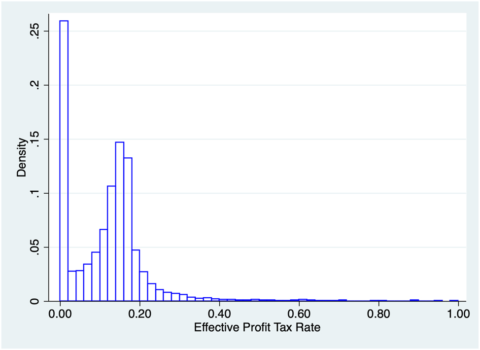
In this section, we document relevant tax facts about Chile. In Chile, all firms are subject to the same statutory tax rate, regardless of their level of profits. The ENIA collects plant-level data on net accounting profits and profit tax expenses. Using these two variables, we calculate the effective tax rate that each firm faces in a given year as the ratio between profit tax expenses and gross accounting profits.^[6]

Figure 1 shows the distribution of effective profit tax rates for 2003, which we have used as an example year, as the distributions for all the years in our sample portray similar characteristics. In particular, four important features characterize the distributions of effective profit tax rates for each year in our time-window of analysis. First, a large number of firms face a 0 percent tax rate (around 30 percent for all years in our sample). This feature is mainly driven by the tax code exemption that specifies that firms with non-positive accounting profits face a corporate tax rate equal to 0 percent.^[7] Second, there is a large concentration of firms with effective tax rates around the statutory tax rate, as seen in Figure 1.^[8] Third, in Table 1 we document that close to 70 percent of plants have an effective tax rate below or equal to the statutory tax rate. Last, the effective profit tax rate that firms face has considerable dispersion, as depicted in Figure 1 as well as the last column of Table 1. Several exemptions outlined in the Chilean tax law, as well as fines for late payments and tax base revaluations to match economic activity with financial payments potentially generate dispersion in effective profit tax rates, as most firms have effective rates that differ from the statutory rate.

Figure 1:

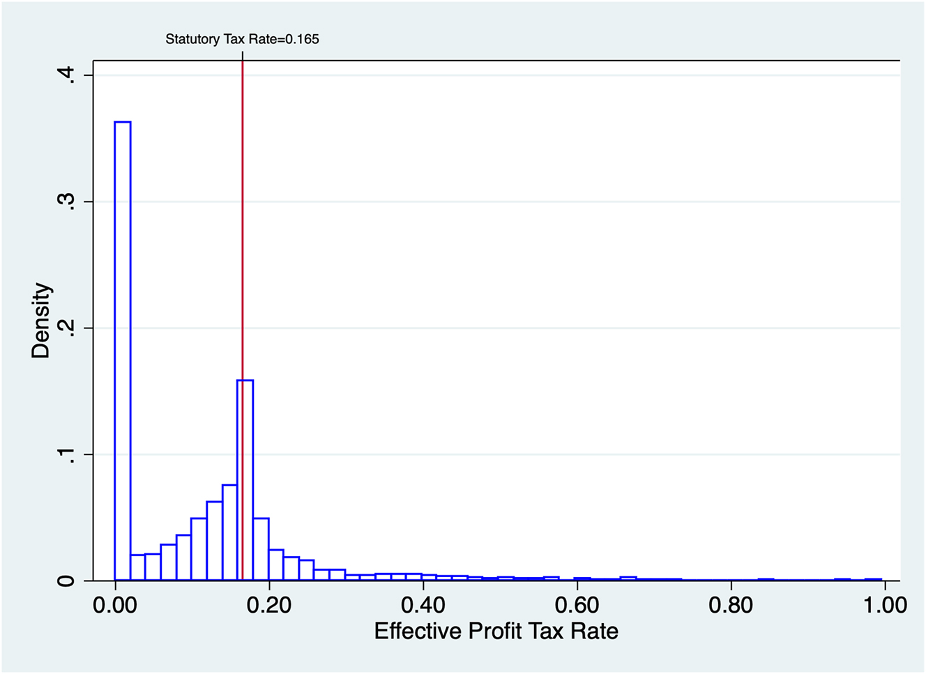
Distribution of effective profit tax rates (2003).

A plant may face an effective tax rate lower than the statutory tax due to several exemptions included in the tax code. For example, plants can deduct unlimited previous years’ losses from their current earnings (unlimited loss carryforward).^[9] These losses are adjusted by cost of living. There are multiple expensing deductions. Plants can expense the cost of scientific investigation and technology either in the current year or up to six consecutive years after the expense has been incurred. Plants can also expense promotional and other expenses geared towards introducing new products and can prorate this expense in three consecutive years. There are also tax credits. Plants that pay the tax have a 4 percent tax credit of physical capital acquired during the fiscal year up to a maximum determined in the tax code. Other exemptions include different types of depreciation depending on the type of asset, and other expensing schemes.

Plants that face an effective tax rate that is higher than the statutory tax rate do so mainly for two reasons: late payment fines and tax base revaluations. Late payment fines range from 10 percent to 30 percent depending on how long it takes the plant to pay the amount owed. Plants also pay 1.5 percent interest per month on their debt. Taxes paid by tax base revaluations are technically called “deferred taxes”. These tax base revaluations arise from analyzing the differences, mostly temporary, between taxable and accounting profit.

The last column of Table 1 presents the standard deviation of effective corporate tax rates for every year of our sample. As mentioned previously, exemptions, deductions, and deferrals inherent to the Chilean tax code allow firms to have effective tax rates that are different than the statutory tax rate, resulting in dispersion in effective rates. To understand whether this dispersion is driven either by innate firm ability to utilize the tax code to reduce their tax burden over time (i.e. firm fixed effect), exemptions targeted at specific firm groups (i.e. region, industry, among others), or idiosyncratic variation, we carry out the following exercise. Using the unbalanced panel of firms between 1998 and 2007, we first regress effective profit tax rates on firm fixed effects and find that 41 percent of the variation in effective tax rates is explained by these fixed effects. Hence, a considerable fraction of the variation of effective profit tax rates is explained by firms’ innate ability to use exemptions in the tax code in order to modify their tax base over time.

To determine whether the remaining variation in effective tax rates is a result of exemptions targeted at firms, at a very granular level, we then regress the residual effective tax rates (residuals of the first regression) on firm size, region, business entity type, and industry, including the interactions between these variables.^[10] Table 9 in the appendix reports the R ² of this exercise across years. Our results show that most of the dispersion in the residual effective profit tax rates is idiosyncratic as exemptions that are targeted according to size, region, entity type, industry, or firm clusters defined by combinations of these variables, explain only between 3 percent and 5 percent of the variation in residual effective tax rates.

3.1 Monopolistic Competition Model

We consider a static monopolistic competition model with heterogeneous firms. We assume a small open economy where the world interest rate r is given and all changes in aggregate capital are due to inflows into the economy. Aggregate labor supply L ̄ is assumed to be inelastic. There is a single final good Y produced by a representative firm in a perfectly competitive output market. The representative firm’s production function is a Cobb-Douglas aggregator, and it uses output Y _s of industries s ∈ 1 , … , S as inputs:

and P _s is the price of industry s.

Industry output is a CES aggregator of M _s differentiated products with elasticity parameter σ:

Differentiated product firms are monopolists over their variety and are heterogeneous in their physical productivity, A _si . Their production function is given by

where K _si and L _si are the capital and labor inputs, respectively, and α _s is the capital share of industry s.

These firms maximize economic profit, which is the sum of accounting profit and the opportunity cost of capital, while facing a corporate tax policy. We make the distinction between economic and accounting profits, since the latter constitutes firms’ net income for tax purposes.^[11] The corporate tax policy is explicitly modeled as follows: if a firm’s accounting profit is positive, it faces a profit tax rate denoted by t _si ≥ 0. Conversely, if a firm’s accounting profit is non-positive, its profit tax rate is 0. This modeling feature incorporates a specific exemption common to many tax systems, including the Chilean system, wherein firms with non-positive accounting profits face a 0 percent corporate tax rate.^[12]

Given the corporate tax policy, a firm chooses capital, K _si , labor, L _si , and its differentiated good’s price, P _si , to maximize economic profit:

where π s i t is the economic profit of a firm that faces profit tax rate t _si , conditioned on positive accounting profit, and π s i 0 is the economic profit of a firm that faces a profit tax of 0, conditioned on non-positive accounting profit. We express accounting profit as:

where δ is the depreciation rate, λ is the fraction of capital that is financed by debt and Γ _si is non-operational income net of non-operational costs.^[13]

Economic profit for a firm facing profit tax rate t _si , subject to positive accounting profit is:

The Lagrange multiplier for the accounting profit’s non-negativity constraint is denoted as μ s i t . The firm-specific output and capital wedges are denoted by τ _Ysi and τ _Ksi , respectively. Maximization yields the following first-order conditions:

Economic profit for a firm facing a 0 percent profit tax rate, subject to non-positive accounting profit is:

The Lagrange multiplier for the accounting profit’s non-positivity constraint is denoted as μ s i 0 . Maximization yields the following first-order conditions:

Section C.1 in the appendix derives the explicit solutions of firms’ optimal choices of K _si , L _si , and P _si .

Similar to Hsieh and Klenow (2009) and Foster, Haltiwanger, and Syverson (2008), we define revenue-based factor productivity as TFPR _si ≡ P _si A _si . Under a Cobb-Douglas production function, this can be expressed as:

From Equations (5)–(8), we observe that firms’ marginal products differ when they face different wedges and profit tax rates. The output wedge distorts firms’ output decisions, as it affects the firms’ marginal products in the same proportion. On the other hand, the capital wedge distorts decisions of capital relative to labor. Importantly, we assume that tax rates do not affect capital and output wedges. However, the tax rate interacts with the wedges in the marginal products of the firm. If we were to set wedges and taxes to zero, then all firms would have the same marginal products. Given this, Equation (9) shows that revenue productivity would also equalize across firms. On the contrary, when firms face different wedges and profit taxes, there is dispersion in revenue productivity. Furthermore, firms with higher TFPR _si are those that have higher wedges, raising their marginal products and lowering their capital, labor, and output levels.

Using the above framework, we construct the aggregate measures for capital, labor, TFP, and output. First, we express the equilibrium allocations for sectoral resources, K _s and L _s , as:

where K = ∑ s = 1 S K s is aggregate capital, L = ∑ s = 1 S L s is aggregate labor, ω s K is the sectoral share of capital, and ω s L is the sectoral share of labor. Sectoral shares have the following expression:

where M R P K ̄ s and M R P L ̄ s are the industry-weighted average of firms’ marginal product of capital and marginal product of labor.^[14]

We derive industry productivity as:

where T F P R ̄ s is the industry-weighted average of firms’ revenue productivity.

Last, aggregate output can be expressed as a function of K _s , L _s , and TFP _s :

Section C.2 in the appendix describes the computation of this model’s equilibrium.

3.2 Calibration and Measurement

We follow an approach similar to Hsieh and Klenow (2009) in our calibration. That is, we set the rental rate of capital to r = 0.05 and the depreciation rate to δ = 0.05. The elasticity of substitution between varieties is fixed at σ = 3, so that firms’ price is 50 percent higher than their marginal cost. In Section 5.1, we evaluate the sensitivity of our results with respect to these assumptions. The capital share α _s in industry s is equal to 1 minus the labor share in that corresponding industry for the United States.^[15] These shares are obtained from the NBER Productivity Database.^[16]

We use the data described in Section 2.1 to measure firms’ average tax rates, output and capital wedges, and revenue and physical productivities. Industries in the model correspond to the four-digit industries within the manufacturing sector according to the ISIC Rev. 3 industry classification.^[17] We measure firms’ value added, P _si Y _si , as the difference between gross revenue and intermediate inputs. We use four-digit industry deflators for gross revenue and intermediate inputs, provided by the data set, to deflate our estimate of firms’ value added. Industry value added, P _s Y _s , is measured as the sum of all firms’ value added within industry s. The capital input, K _si , is measured as the book value of fixed assets, which we deflate using the gross revenue deflators. To control for differences in human capital, hour requirements, and rent sharing across plants, we follow Hsieh and Klenow (2009) and use the wage bill deflated by the intermediate input industry deflator as the measure for labor, L _si . In a robustness check, we also consider hours worked for our measure of labor.^[18]

As described above, we calculate effective tax rates as the ratio between a firm’s profit taxes and its gross accounting profits. We denote the measured firm-specific average tax rate as t ̂ s i and use it as firm i’s marginal tax rate in our benchmark quantitative exercises. The main drawback of this approach is that the observed average tax rate may be an imprecise proxy of a firm's marginal tax rate. Studies by Graham (1996), Plesko (2003), and Graham and Mills (2008) suggest that simulated tax rates offer more accurate approximations of firms’ marginal tax rates compared to average tax rates. However, as posited by Shevlin (1999), the appropriateness of using average tax rates as proxies for marginal tax rates depends on the specific research question. Moreover, Devereux and Griffith (2003) argue that average tax rates may be significant for investment decisions, particularly in contexts where firms face credit constraints, such as in developing countries like Chile. We aim to quantify the allocative efficiency impact of the Chilean corporate tax code. As such, the main advantage of using the average tax rate is that it incorporates all exemptions and deductions of the tax code into our tax rate measure. Nevertheless, to address the potential mismeasurement of the marginal tax rate, we conduct several robustness checks in Section 6 to ensure that our results are not driven by our choice of the marginal tax rate proxy.

Using the data and parameter values described above, we back out the capital and output wedges in the following manner. For firms with positive accounting profits, we use Equations (5) and (6) to obtain the firm-specific wedges. Since μ s i t = 0 , the output and capital wedges are:

On the other hand, for firms with negative accounting profits the capital and output wedges are obtained from Equations (7) and (8). In this case, μ s i 0 = 0 and the wedges are:^[19]

Last, we use Equations (3) and (9) to calculate firms’ physical productivity, A _si , and revenue productivity, TFPR _si , respectively.^[20] Using Equations (10)–(15), we construct industry and aggregate measures of output, productivity, capital, and labor.

4.1 Output Gap Decomposition

To study the impact of different tax policies, it is convenient to define the output gap between two economies that only differ in the wedges and effective tax rates each firm faces. We decompose this gap into five objects: the TFP gap, intersectoral capital reallocation, intersectoral labor reallocation, change in aggregate capital, and change in aggregate labor. The TFP gap reflects changes in intrasectoral allocative efficiency (i.e. intrasectoral reallocation of resources), as can be seen from Equations (9) and (14). Capital and labor intersectoral reallocation are also affected by tax rates and wedges since the industry shares of capital and labor, ω ^K and ω ^L , are a function of firms’ marginal products. Aggregate capital demand changes for different tax rates and wedges through the marginal cost of capital. Last, in equilibrium aggregate labor demand equates aggregate labor supply, and given that aggregate labor supply is fixed, the change in aggregate labor is always zero between any two economies that differ in firm wedges and firm effective tax rates.

Consider two economies that have different firm-specific output and capital wedges and profit tax rates but are equal in all other aspects. Denote the levels of output of these two economies by Y and Y ̃ . We refer to the output gap as the log percentage difference between these two levels of output. Using Equations (10), (11), and (15), the output gap can be decomposed as follows:

Below, we analyze the output and TFP gaps between different counterfactual tax rates policies and the observed Chilean economy.

4.2 Output and TFP Gains from Eliminating Corporate Taxation

In this section, we quantify the output gap decomposition using Equation (20). We consider two economies that differ only in the corporate tax policy implemented. Both economies are subject to the same firm-specific output and capital wedges. By doing this, we ensure that firms face the same frictions implied by the data in both economies. In one economy, we set taxes to t _si = 0, regardless of firms’ level of accounting profits, and, in the other economy, we set taxes to the observed firm-specific average tax rates, t s i = t ̂ s i , i.e. the observed Chilean economy. This measures the change in output implied by modifying the actual Chilean tax policy to one with no corporate taxation, allowing us to quantify the effect of the dispersion and level of the observed tax rates on TFP.

Table 2 presents the results from the output gap decomposition. Moving to a counterfactual scenario with no corporate tax rates generates an increase in output that ranges from 20 percent to 38 percent, depending on the year considered. In all of the years analyzed, TFP increases due to the policy change. This increase ranges from 4 percent to 11 percent and is due to a more efficient intrasectoral allocation of resources. The effect on intersectoral reallocation is small. Intersectoral allocation of capital accounts for between −3 percent and 2 percent of the change in output. In three years, the effect of intersectoral allocation of capital is negative. Intersectoral allocation of labor increases in all years but only between 0 percent and 2 percent. Most of the change in the output gap is generated by large increases in the demand for aggregate capital. This is an implication of the small open economy assumption of the model. Setting t _si = 0 directly changes the cost of capital, which in this case generates large inflows of capital into the economy. Last, since aggregate labor supply is inelastic, the change in aggregate labor is always zero for any counterfactual policy scenario. Hence, we do not report this change in Table 2.

4.3 Allocative Efficiency Gains and Corporate Tax Rates

In this section, we analyze the allocative efficiency impact of different levels of profit tax rates by examining a series of counterfactual flat tax rate policies. Our approach involves implementing counterfactual exercises where firms operate under corporate tax policies that apply a uniform flat tax rate, t s i = t ̄ , if their accounting profits are positive. If their accounting profits are non-positive, firms face a 0 percent tax rate. In these counterfactual scenarios, all firms face the same output and capital wedges implied by the data. We compare these counterfactual economies to the observed Chilean economy and measure changes in intrasectoral allocative efficiency with respect to the data.

Equations (5)–(8) portray the mechanisms through which intrasectoral reallocation of resources occurs due to these counterfactual tax policies. Profit tax rates affect the dispersion of firms’ marginal products in two ways. Firstly, dispersion in profit tax rates directly leads to heterogeneous marginal products. Secondly, the level of profit tax rates indirectly impacts the dispersion of marginal products through its interaction with firm-level wedges. Higher variance in marginal revenue products results in higher dispersion in revenue productivity, thereby depressing TFP. In the counterfactual economies, the only source of dispersion in corporate tax rates stems from the exemption considered within the theoretical model, wherein firms with non-positive accounting profits are subjected to a 0 percent tax rate. In contrast, the dispersion in corporate tax rates for the observed Chilean economy reflects all the exemptions and deductions of the tax system. Consequently, the counterfactual scenarios are anticipated to exhibit less dispersion in profit tax rates compared to the observed Chilean economy, as the latter accounts for all exemptions under the Chilean tax system. However, this does not imply that across all counterfactual scenarios, dispersion in marginal products and revenue productivity would be lower, due to the interaction between the counterfactual tax rate levels and the existing firm-level wedges. Hence, these counterfactual flat profit tax rate policies have the potential to either enhance or diminish intrasectoral allocative efficiency.

The schedule in Figure 2 portrays the TFP gap between a counterfactual corporate tax policy with t s i = t ̄ and the observed Chilean economy t s i = t ̂ s i , for different levels of t ̄ , in the year 2003. This graph shows that the TFP gap decreases monotonically with the level of the tax rate, t ̄ . This is the case for all the years studied in our sample. Furthermore, for lower levels of t ̄ , the TFP gap is positive (TFP gains), while for higher levels of t ̄ , this TFP gap becomes negative (TFP loss). In 2003, a flat tax rate policy of t ̄ = 9.76  percent would have generated the same aggregate TFP level as the one implied by the observed firm-specific corporate tax rates. This flat tax rate is lower than 16.5 percent, which was the statutory tax rate for that year. If in 2003 Chile had applied a flat tax rate policy at the statutory tax rate level to all firms with positive accounting profits, the loss in TFP would have been 2.46 percent. This remark is consistent for all the years in our sample.

Figure 2:

Relationship between TFP gap and t ̄ (2003).

The monotonically decreasing relationship between the level of the uniform tax rate policy and the TFP gap can be rationalized as follows. As expected, the profit tax rate dispersion in the observed Chilean economy exceeds that of all the counterfactual economies studied. In 2003, the dispersion of profit tax rates in the observed Chilean economy was 13.44 percent, while in the counterfactual economies, it ranged from 0 percent ( t ̄ = 0  percent ) to 8.99 percent ( t ̄ = 20  percent ) . The lower tax rate dispersion in the counterfactual economies translates into lower dispersion in firms’ revenue productivity, leading to TFP gains in these counterfactual scenarios relative to the observed Chilean economy. However, two mechanisms cause these gains to diminish as the counterfactual uniform tax rate level rises. First, as previously explained, the higher the level of the counterfactual flat tax rate, the more it amplifies the distortions embedded in the output and capital wedges. Second, as the uniform tax rate level increases, tax rate dispersion rises in the counterfactual economies. We find that the deviations from the mean tax rate increase in absolute value as the counterfactual flat tax rate level rises, thereby increasing tax rate dispersion. Additionally, economies with higher flat tax rate levels have more firms with a 0 percent tax rate compared to economies with lower counterfactual flat tax rate levels, resulting in higher tax rate dispersion.^[21] Consequently, these two mechanisms offset the gains from eliminating the observed Chilean economy’s higher tax rate dispersion. This is because these mechanisms increase the variance of firms’ marginal products, which yields higher revenue productivity dispersion. The dispersion in marginal products and revenue productivity for counterfactual policy scenarios t s i = t ̄ relative to the observed Chilean economy is illustrated in Figure 3. For low levels of the flat tax rate, the dispersion in firms’ revenue productivity is lower in the counterfactual scenarios relative to the observed Chilean economy, aligning with higher TFP in the counterfactual scenarios. However, as the tax rate level increases, the dispersion of revenue productivity increases due to the described mechanisms, leading to increased misallocation and resulting in TFP losses for high levels of the flat tax rate.

Figure 3:

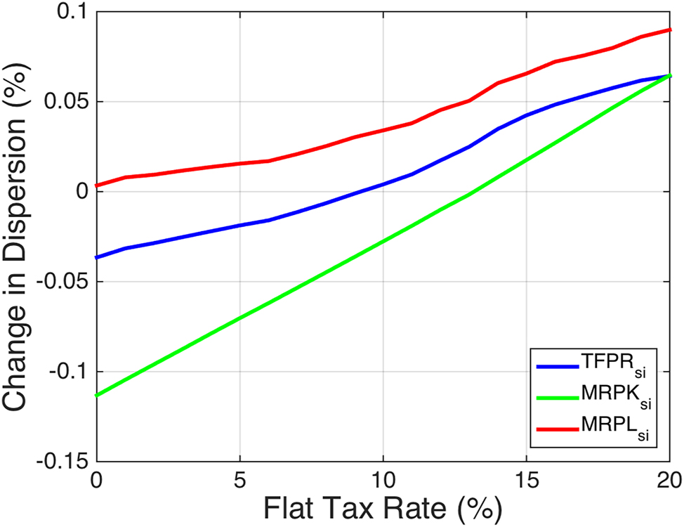
Change in dispersion measures relative to t ̄ (2003). Notes: The change in dispersion for revenue productivity is measured as the log difference between the standard deviation of revenue productivity implied by the flat tax rate policy and the standard deviation of revenue productivity implied by the observed tax rates. The same statistic is calculated for marginal revenue products.

To corroborate our results, we perform an alternative measure of allocative efficiency similar to Olley and Pakes (1996). Our results are summarized in Figure 4. In Panel (a), the schedule labeled “Counterfactual Policy” plots the correlation between firm productivity, A _si , and the share of firm i’s capital stock, K _si , in sector s’s capital stock, K _s , for different flat tax rate levels t ̄ . Panel (b) plots the correlation between firm productivity, A _si , and the share of firm i’s labor, L _si , in sector s’s labor, L _s , for different flat tax rate levels t ̄ . The dotted line labeled “Data” corresponds to the correlation measures for the observed Chilean data in 2003. The correlation of firm productivity with respect to both capital and labor share drops as flat tax levels increase, which shows that the intrasectoral reallocation mechanisms described above drive the fall in the TFP gap. More resources are being allocated toward less productive firms.

Figure 4:

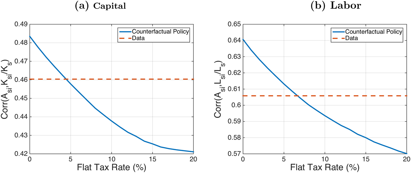
Correlation between firm productivity and activity share (2003). Notes: The solid blue line labeled “counterfactual policy” corresponds to the correlation between firm productivity and firm activity share for different levels of t ̄ . The dotted orange line labeled “data” corresponds to the correlation between firm productivity and firm activity share in the data.

Next, we analyze the effect of these tax policies on government revenue. In Figure 5, the blue schedule labeled “Counterfactual Policy” portrays the Laffer curve for different flat tax rate policies. A clear trade-off stands out. Although very low flat tax rates yield higher levels of TFP, government revenue from corporate taxation is smaller. The dotted line labeled “Data” is the government revenue collected from the observed corporate tax rates. The flat tax rate policy that yields the same revenue is t ̄ = 7.97 percent. If this policy had been implemented in Chile in 2003, then TFP would have increased by 0.77 percent. This pattern, however, is not found for all years in our sample. For some years in our sample, the revenue-neutral flat tax rate policy generates TFP gains with respect to the data, while for others it generates TFP losses.

Figure 5:

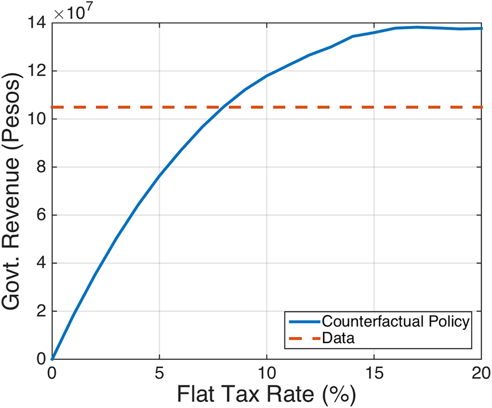
Relationship between government revenue and t ̄ (2003). Notes: The solid blue line labeled “counterfactual policy” corresponds to the government revenue for different levels of t ̄ . The dotted orange line labeled “data” corresponds to the government revenue implied by the observed effective tax rates.

5.1 Sensitivity to Parameter Values

Table 3 shows the TFP gap from eliminating corporate taxes for different interest rates r, depreciation rates δ, and values of σ, the parameter of the elasticity of substitution across varieties. For different interest rates, results are identical to the benchmark. As seen in Equation (4), when λ = 0, the interest rate r does not affect the accounting profits of firms. Hence, it does not interact with the corporate tax rate in the marginal revenue products, as shown in Equations (5)–(8). For this reason, different interest rates do not affect the TFP gap when corporate tax rates are eliminated. This is not the case anymore when we consider different values of λ.

On the other hand, the depreciation rate has a direct impact on accounting profits, regardless of the value of λ. Moreover, as the depreciation rate increases, the TFP gains from eliminating corporate taxes are higher. Finally, we have chosen a conservative σ at the low end of the empirical estimates. Under σ = 5, the TFP gains are higher from eliminating corporate taxation.

As in Section 4.3, we carry out the same flat tax rate policy counterfactuals. Our results are robust when we consider different parameter values for r, δ, and σ. Figure 6 shows the same decreasing relationship between the TFP gap and the level of the flat tax rate, t ̄ , as observed in Figure 2.

Figure 6:

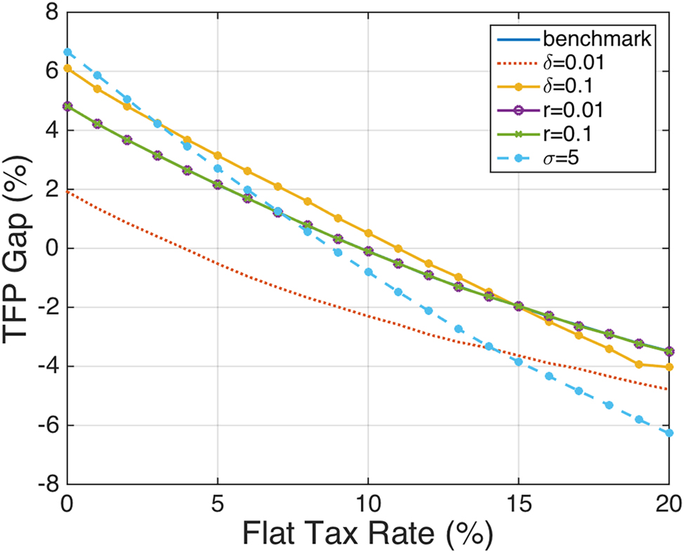
Relationship between TFP gap and t ̄ : parameter sensitivity (2003).

5.2 Hours Worked as Input for Labor

In the results described above, we measure L _si as the firm’s wage bill. As a robustness check, we recalculate our estimates using hours worked as labor input.^[22] Similar to Hsieh and Klenow (2009), using the wage bill for the labor input allows us to control for between-firm heterogeneity in rent sharing, skill level, and hours worked requirements. As these differences are not modeled in our framework, when we use hours as labor input, they are loaded into the output and capital wedges. As a result, dispersion in TFPR _si is higher.

Repeating our exercise with hours as labor input yields two main findings. First, in line with the results in Section 4.3, the TFP gap falls when we increase the level of the flat corporate tax rate in the counterfactual economies, as seen in Figure 7. Second, the TFP gap across different counterfactual policies is larger. This is because our results are amplified since the corporate tax rate interacts with output and capital wedges, which are more dispersed for the reasons mentioned at the beginning of this section. This result holds across all years of our sample, as seen in the output gap decomposition in Table 10 in the appendix.

Figure 7:

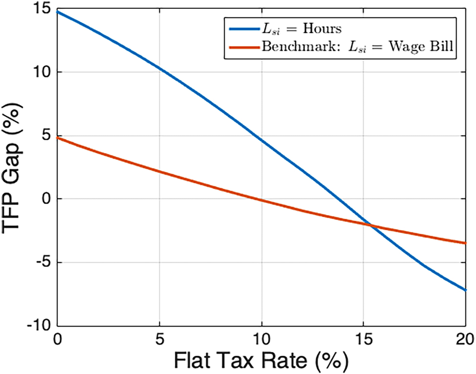
Relationship between TFP gap and t ̄ : hours as labor input (2003). Notes: Benchmark corresponds to the results of Figure 2.

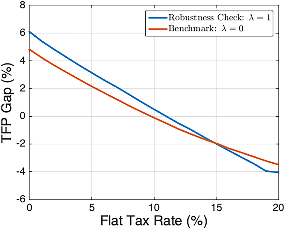
6.1 Financing Capital with Debt

So far, we have assumed that capital is financed entirely with equity, λ = 0. This is a strong assumption since firms may finance capital with a mix of capital and debt. Firms have incentives to finance capital with debt since interest payments are discounted from accounting profits and therefore lower the tax that firms must pay. In this section, we analyze the other extreme case in which all capital is financed with debt λ = 1 to determine whether our results are sensitive to this assumption. Note that our calculation of the effective tax rate that firms face is not affected by the capital structure decision of the firm since we observe profits net of interest and taxes. Hence, the tax rate we calculate already takes into account the firm’s capital structure. However, our results will vary depending on the amount of capital a firm finances with debt, since λ interacts with the effective tax rate t _si in the marginal revenue product of capital.

Note that if we observed profits before subtracting interest and taxes instead of using profits net of interest and taxes, differences in access to credit and other distortions that may affect the capital structure would also be loaded into the effective tax rate instead of the capital and output wedges. Also, it is important to note that the fraction of capital financed with debt can potentially be firm specific. For example, some firms may have better access to credit than others. Uras (2014) explores this mechanism and finds that it has important implications for capital misallocation. In our setup, these differences in access to credit are reflected in the capital and output wedges.

Table 4 shows the output gap decomposition under λ = 1 and under the scenario in which corporate tax rates are equal to t _si = 0. Results are very similar to those of Table 2. The increase in output from eliminating the effect of dispersion and level of corporate taxes is mainly explained by an increase in aggregate capital demand and an increase in TFP. Hence, we can see that intrasectoral reallocation of resources plays a significant role in explaining the output gap, while intersectoral reallocation of resources has a negligible effect on the output gap. This finding is consistent with the results found in Section 4.2.

As in Section 4.3, we carry out different counterfactual flat tax rate policies and evaluate their relationship to the TFP gap. In Figure 8 we can observe that results are similar under the scenario in which all capital is financed by debt, λ = 1, and under the benchmark scenario in which capital is financed by equity, λ = 0. That is, as the flat tax rate level increases, the TFP gap falls. Also under the assumption that λ = 1, the dispersion of marginal products and revenue productivity increases as the flat tax rate levels increase. Higher flat tax rates exacerbate the effect of the output and capital wedges and also create higher tax rate dispersion in comparison to lower flat tax rates. As in Section 4.3, these two mechanisms increase revenue productivity dispersion as the flat tax rate rises, which indicates that resources are reallocating from more productive firms to less productive firms.

Figure 8:

Relationship between TFP gap and t ̄ : λ = 1 (2003). Notes: Benchmark corresponds to the results of Figure 2.

6.2 Statutory Tax Rate as the Marginal Tax Rate

The literature, including papers by Graham (1996), Plesko (2003), Graham and Mills (2008), among others, has highlighted concerns regarding the accuracy of average tax rates as estimates of firms’ marginal tax rates, proposing various alternative proxies. To address this issue, this section examines one such alternative: the statutory tax rate. Similar to Graham (1996) and Djankov et al. (2010), we use the statutory tax rate as a marginal tax rate proxy. For this, we recalibrate the benchmark economy under the following corporate tax policy: firms with positive profits face the statutory tax rate, while those with non-positive profits face a 0 percent tax rate. Subsequently, we contrast this alternative benchmark economy with a counterfactual scenario in which corporate taxation is entirely eliminated.

Table 5 presents the output gap resulting from eliminating the effects of both the dispersion and level of corporate taxes, relative to the alternative benchmark. The findings closely mirror those of Table 2. The rise in output attributed to the removal of corporate taxation primarily stems from an increase in aggregate capital demand, followed by improved intrasectoral allocative efficiency (TFP Gap), while the impact of intersectoral reallocation of resources on the output gap remains minimal. In this robustness exercise, intrasectoral efficiency gains range from 7 to 12 percent across all years in our sample, aligning closely with the estimates of the benchmark calibration, which range from 4 to 11 percent across all years in the sample. It is important to note that in this robustness exercise, the estimated output and capital wedges that rationalize observed firms’ input choices, differ from the wedges derived in the benchmark calibration due to the different marginal tax rate proxy. As a result, the dispersion in corporate tax rates resulting from all the tax code’s exemptions not considered in our theoretical framework is now attributed to other distortions in the economy rather than solely to the Chilean Tax Code.^[23]

6.3 Accounting for Loss Carryforward

One of the exemptions that may generate dispersion in effective corporate tax rates is the fact that plants can carry forward losses from one period to the next to reduce their tax base. Our results in Section 2.2 show that firm fixed effects account for a considerable fraction of the variation of effective corporate tax rates. Firm fixed effects capture plants’ ability to utilize the tax code to the modify their tax base, through exemptions like loss carryforward. In particular, firms optimally choose capital and labor taking into account that this exemption allows them to reduce their tax burden. However, we do not model this explicitly since our analysis is static, and thus this specific source of distortion is loaded into the wedges. To measure how sensitive our results are to this omission, we consider the following exercise. We take the average across years for each plant’s relevant variables and estimate the TFP gap for our policy counterfactuals. By doing this, any losses that could have been carried forward will smooth out. Note that if all the dispersion in effective tax rates was due to this channel, the tax rates that firms face in this exercise should be less dispersed and similar to the statutory rate. This is not the case, however, as the effective tax rate calculated by averaging profit and profit tax across years is distributed similarly to the effective tax rates calculated year by year. We can see this by comparing Figures 1 and 9.

Figure 9:

Distribution of effective profit tax rates – loss carryforward (2003).

Our results for this exercise are similar to our benchmark results. The decomposition of the output gap when firms face t _si = 0 can be seen in Table 11 in the appendix. When firms do not face corporate tax rates, TFP increases by 6.18 percent, which is within the range of values of our benchmark analysis, as seen in Table 2. Hence, loss carryforward is not the main driver of the distortions generated by heterogeneous tax rates. Similar to Section 4.2, intersectoral reallocation of resources accounts for a very small portion of the output gap, while changes in aggregate capital demand play a more significant role.

As in the benchmark, we also carry out flat tax rate counterfactual policies and measure their effect on aggregate TFP. We find that the negative relationship between the TFP gap and the flat tax rate level still persists, as seen in Figure 10. Hence, despite eliminating the dispersion in corporate tax rates coming from loss carryforward, as the flat tax rate increases, resources are reallocated from more efficient firms to less efficient firms.

Figure 10:

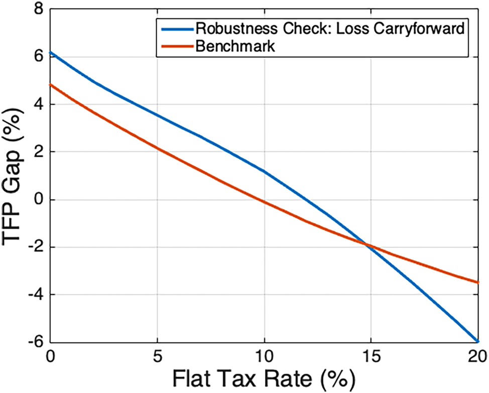
Relationship between TFP gap and t ̄ : loss carryforward (2003). Notes: Benchmark corresponds to the results of Figure 2.

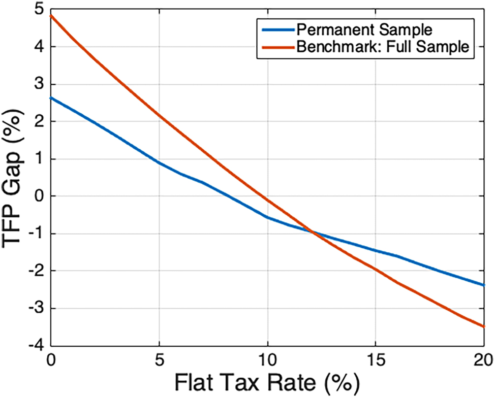
6.4 Permanent Sample

Dispersion in corporate tax rates can potentially be driven by tax exemptions given to young entrant firms, which are usually directed at fostering industry competition. If this is the only source of tax rate dispersion and entrant firms are relatively less productive than incumbent firms, then these tax exemptions would be responsible for the positive TFP gap shown in Table 2. Intuitively, these tax exemptions would be allocating more resources to less productive entrant firms and fewer resources to more productive incumbent ones. Hence, if Chile moved to a tax policy with no corporate taxes, then resources would reallocate to the more productive incumbent firms, generating the positive TFP gap.

To control for this mechanism, we focus on the firms that were always in operation for the period 1998 to 2007 and then perform the output gap decomposition for the years 2003–2007. By doing this, we make sure that the firms had been in operation at least five years.^[24] If the only source of tax rate dispersion was exemptions to less productive entrant firms, then when we eliminate them from the sample, the TFP gap would be 0. This is not the case, however, as can be seen in Table 6, which implies that there are other sources of corporate tax rate dispersion that generate a positive TFP gap. In this exercise, we also control for the fact that less productive exiting firms are driving our results, since the permanent sample comprises highly productive firms that have been operating for at least 10 years.

As shown in Table 12 in the appendix, there is significant dispersion in the effective corporate tax rates faced by the firms in the permanent sample for all years. Hence, tax exemptions given to young firms are not the main driver of this dispersion.

By comparing Tables 6 with 2, we can see that the results for intersectoral reallocation of resources and changes in input demands are similar. Also, we can observe that the TFP gap from eliminating corporate taxes is smaller in the permanent sample in comparison to the whole sample. The main reason for this finding is that the permanent sample controls for firm entry and exit. Firms in this sample had been in operation for at least 10 years in 2007. Hence, they were relatively more productive than the firms that entered or exited the sample during the time period we analyze. We document this finding in Figure 11, in which we compare the distribution of log A s i for the whole sample in comparison to the permanent sample for 2003.

Figure 11:

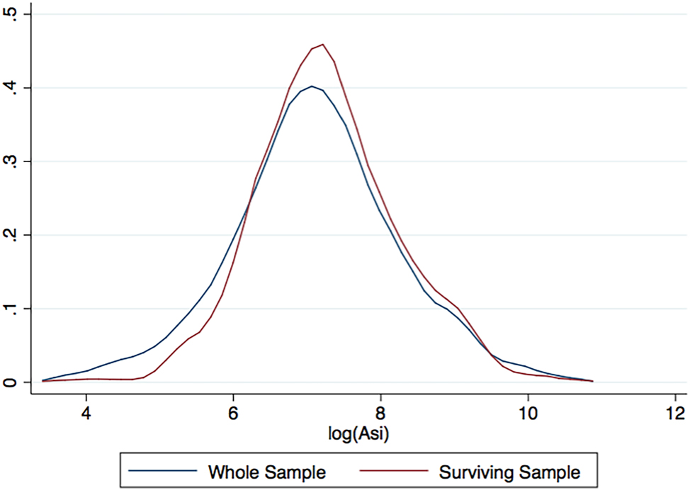
Distribution of log A s i for the whole and permanent samples.

We find that the mean of log A s i is higher in the permanent sample in comparison to the whole sample. Moreover, the distribution of the permanent sample has a much thinner left tail and is more concentrated around the mean. This pattern occurs in all the years between 1998 and 2007. This is evidence that the firms that exit every year tend to be the least productive firms, while the more productive firms remain. As a result, the gains from reallocation of resources in the permanent sample are smaller than in the whole sample.^[25] Last, it is important to note that for the permanent sample, the TFP gap is also decreasing in the level of flat tax rates, as seen in Figure 12 in the appendix.

References

Ábrahám, Árpád, Piero Gottardi, Joachim Hubmer, and Lukas Mayr. 2023. “Tax Wedges, Financial Frictions and Misallocation.” Journal of Public Economics 227: 105000. https://doi.org/10.1016/j.jpubeco.2023.105000.Search in Google Scholar
Altshuler, Rosanne, and Alan J. Auerbach. 1990. “The Significance of Tax Law Asymmetries: An Empirical Investigation.” Quarterly Journal of Economics 105 (1): 61–86. https://doi.org/10.2307/2937819.Search in Google Scholar
Asker, John, Allan Collard-Wexler, and Jan De Loecker. 2014. “Dynamic Inputs and Resource (Mis)Allocation.” Journal of Political Economy 122 (5 (October): 1013–63. https://doi.org/10.1086/677072.Search in Google Scholar
Auerbach, Alan J. 1986. “The Dynamic Effects of Tax Law Asymmetries.” The Review of Economic Studies 53 (2): 205–25. https://doi.org/10.2307/2297647.Search in Google Scholar
Auerbach, Alan J. 2002. “Taxation and Corporate Financial Policy.” Handbook of Public Economics 3: 1251–92.10.1016/S1573-4420(02)80023-4Search in Google Scholar
Auerbach, Alan J. 2018. “Measuring the Effects of Corporate Tax Cuts.” The Journal of Economic Perspectives 32 (4): 97–120. https://doi.org/10.1257/jep.32.4.97.Search in Google Scholar
Buera, Francisco J., Joseph P. Kaboski, and Yongseok Shin. 2011. “Finance and Development: A Tale of Two Sectors.” The American Economic Review 101 (5): 1964–2002. https://doi.org/10.1257/aer.101.5.1964.Search in Google Scholar
Caggese, Andrea, Vicente Cuñat, and Daniel Metzger. 2019. “Firing the Wrong Workers: Financing Constraints and Labor Misallocation.” Journal of Financial Economics 133 (3): 589–607. https://doi.org/10.1016/j.jfineco.2017.10.008.Search in Google Scholar
Calcagnini, Giorgio, Germana Giombini, and Enrico Saltari. 2009. “Financial and Labor Market Imperfections and Investment.” Economics Letters 102 (1): 22–6. https://doi.org/10.1016/j.econlet.2008.10.005.Search in Google Scholar
Cingano, Federico, Marco Leonardi, Julian Messina, and Giovanni Pica. 2010. “The Effects of Employment Protection Legislation and Financial Market Imperfections on Investment: Evidence from a Firm-Level Panel of EU Countries.” Economic Policy 25 (61): 117–63. https://doi.org/10.1111/j.1468-0327.2009.00235.x.Search in Google Scholar
Cingano, Federico, Marco Leonardi, Julian Messina, and Giovanni Pica. 2016. “Employment Protection Legislation, Capital Investment and Access to Credit: Evidence from Italy.” The Economic Journal 126 (595): 1798–822. https://doi.org/10.1111/ecoj.12212.Search in Google Scholar
Cummins, Jason G., Kevin A. Hassett, R. Glenn Hubbard, Robert E. Hall, and Ricardo J. Caballero. 1994. “A Reconsideration of Investment Behavior Using Tax Reforms as Natural Experiments.” Brookings Papers on Economic Activity 1994 (2): 1–74. https://doi.org/10.2307/2534654.Search in Google Scholar
Da Rin, Marco, Marina Di Giacomo, and Alessandro Sembenelli. 2011. “Entrepreneurship, Firm Entry, and the Taxation of Corporate Income: Evidence from Europe.” Journal of Public Economics 95 (9–10): 1048–66. https://doi.org/10.1016/j.jpubeco.2010.06.010.Search in Google Scholar
Da-Rocha, José-María, Diego Restuccia, and Marina Mendes Tavares. 2019. “Firing Costs, Misallocation, and Aggregate Productivity.” Journal of Economic Dynamics and Control 98: 60–81. https://doi.org/10.1016/j.jedc.2018.09.005.Search in Google Scholar
David, Joel M., Hugo A. Hopenhayn, and Venky Venkateswaran. 2016. “Information, Misallocation, and Aggregate Productivity.” Quarterly Journal of Economics 131 (2): 943–1005. https://doi.org/10.1093/qje/qjw006.Search in Google Scholar
Devereux, Michael P., and Rachel Griffith. 2003. “Evaluating Tax Policy for Location Decisions.” International Tax and Public Finance 10: 107–26. https://doi.org/10.1023/a:1023364421914.10.1023/A:1023364421914Search in Google Scholar
Djankov, Simeon, Tim Ganser, Caralee McLiesh, Rita Ramalho, and Andrei Shleifer. 2010. “The Effect of Corporate Taxes on Investment and Entrepreneurship.” American Economic Journal: Macroeconomics 2 (3): 31–64. https://doi.org/10.1257/mac.2.3.31.Search in Google Scholar
Erosa, Andrés, and Beatriz González. 2019. “Taxation and the Life Cycle of Firms.” Journal of Monetary Economics 105: 114–30. https://doi.org/10.1016/j.jmoneco.2019.04.006.Search in Google Scholar
Foster, Lucia, John Haltiwanger, and Chad Syverson. 2008. “Reallocation, Firm Turnover, and Efficiency: Selection on Productivity or Profitability?” The American Economic Review 98 (1): 394–425. https://doi.org/10.1257/aer.98.1.394.Search in Google Scholar
Gopinath, Gita, Şebnem Kalemli-Özcan, Loukas Karabarbounis, and Carolina Villegas-Sanchez. 2017. “Capital Allocation and Productivity in South Europe.” Quarterly Journal of Economics 132 (4): 1915–67. https://doi.org/10.1093/qje/qjx024.Search in Google Scholar
Gourio, Francois, and Jianjun Miao. 2010. “Firm Heterogeneity and the Long-Run Effects of Dividend Tax Reform.” American Economic Journal: Macroeconomics 2 (1): 131–68. https://doi.org/10.1257/mac.2.1.131.Search in Google Scholar
Graham, John R. 1996. “Proxies for the Corporate Marginal Tax Rate.” Journal of Financial Economics 42 (2): 187–221. https://doi.org/10.1016/0304-405x(96)00879-3.Search in Google Scholar
Graham, John R., and Lillian F. Mills. 2008. “Using Tax Return Data to Simulate Corporate Marginal Tax Rates.” Journal of Accounting and Economics 46 (2–3): 366–88. https://doi.org/10.1016/j.jacceco.2007.10.001.Search in Google Scholar
Graham, John R., Michael L. Lemmon, and James S. Schallheim. 1998. “Debt, Leases, Taxes, and the Endogeneity of Corporate Tax Status.” The Journal of Finance 53 (1): 131–62. https://doi.org/10.1111/0022-1082.55404.Search in Google Scholar
Guner, Nezih, Gustavo Ventura, and Yi Xu. 2008. “Macroeconomic Implications of Size-Dependent Policies.” Review of Economic Dynamics 11 (4): 721–44. https://doi.org/10.1016/j.red.2008.01.005.Search in Google Scholar
Haltiwanger, John, Robert Kulick, and Chad Syverson. 2018. “Misallocation Measures: The Distortion that Ate the Residual,” National Bureau of Economic Research Working Paper 24199 (January).10.3386/w24199Search in Google Scholar
Hopenhayn, Hugo A. 2014. “Firms, Misallocation, and Aggregate Productivity: A Review.” Annual Review of Economics 6 (1): 735–70. https://doi.org/10.1146/annurev-economics-082912-110223.Search in Google Scholar
Hopenhayn, Hugo, and Richard Rogerson. 1993. “Job Turnover and Policy Evaluation: A General Equilibrium Analysis.” Journal of Political Economy 101 (5): 915–38. https://doi.org/10.1086/261909.Search in Google Scholar
Hsieh, Chang-Tai, and Peter J. Klenow. 2009. “Misallocation and Manufacturing TFP in China and India.” Quarterly Journal of Economics 124 (4): 1403–48. https://doi.org/10.1162/qjec.2009.124.4.1403.Search in Google Scholar
Hsieh, Chang-Tai, and Jonathan A. Parker. 2007. “Taxes and Growth in a Financially Underdeveloped Country: Evidence from the Chilean Investment Boom.” Economia 8 (1): 1, https://doi.org/10.1353/eco.2008.0004.Search in Google Scholar
Kaymak, Barış, and Immo Schott. 2019. “Loss-Offset Provisions in the Corporate Tax Code and Misallocation of Capital.” Journal of Monetary Economics 105: 1–20. https://doi.org/10.1016/j.jmoneco.2019.04.011.Search in Google Scholar
Levinsohn, James, and Amil Petrin. 2003. “Estimating Production Functions Using Inputs to Control for Unobservables.” The Review of Economic Studies 70 (2): 317–41. https://doi.org/10.1111/1467-937x.00246.Search in Google Scholar
Liu, Lili. 1993. “Entry-Exit, Learning, and Productivity Change: Evidence from Chile.” Journal of Development Economics 42 (2): 217–42. https://doi.org/10.1016/0304-3878(93)90019-j.Search in Google Scholar
McGrattan, Ellen R., and Edward C Prescott. 2005. “Taxes, Regulations, and the Value of US and UK Corporations.” The Review of Economic Studies 72 (3): 767–96. https://doi.org/10.1111/j.1467-937x.2005.00351.x.Search in Google Scholar
Midrigan, Virgiliu, and Daniel Yi Xu. 2014. “Finance and Misallocation: Evidence from Plant-Level Data.” The American Economic Review 104 (2): 422–58. https://doi.org/10.1257/aer.104.2.422.Search in Google Scholar
Oberfield, Ezra. 2013. “Productivity and Misallocation During a Crisis: Evidence from the Chilean Crisis of 1982.” Special Issue: Misallocation and Productivity. Review of Economic Dynamics 16 (1): 100–19. https://doi.org/10.1016/j.red.2012.10.005.Search in Google Scholar
Olley, G. Steven, and Ariel Pakes. 1996. “The Dynamics of Productivity in the Telecommunications Equipment Industry.” Econometrica 64 (6): 1263–97. https://doi.org/10.2307/2171831.Search in Google Scholar
Petrin, Amil, and Jagadeesh Sivadasan. 2013. “Estimating Lost Output from Allocative Inefficiency, with an Application to Chile and Firing Costs.” The Review of Economics and Statistics 95 (1): 286–301. https://doi.org/10.1162/rest_a_00238.Search in Google Scholar
Plesko, George A. 2003. “An Evaluation of Alternative Measures of Corporate Tax Rates.” Journal of Accounting and Economics 35 (2): 201–26. https://doi.org/10.1016/s0165-4101(03)00019-3.Search in Google Scholar
Poterba, James M., and Lawrence H. Summers. 1984. The Economic Effects of Dividend Taxation. Technical report. National Bureau of Economic Research.10.3386/w1353Search in Google Scholar
Restuccia, Diego, and Richard Rogerson. 2008. “Policy Distortions and Aggregate Productivity with Heterogeneous Establishments.” Review of Economic Dynamics 11 (4): 707–20. https://doi.org/10.1016/j.red.2008.05.002.Search in Google Scholar
Restuccia, Diego, and Richard Rogerson. 2017. “The Causes and Costs of Misallocation.” The Journal of Economic Perspectives 31 (3): 151–74. https://doi.org/10.1257/jep.31.3.151.Search in Google Scholar
Rossbach, Jack, and Jose Asturias. 2017. Misallocation in the Presence of Multiple Production Technologies. 2017 Meeting Papers 1094. Society for Economic Dynamics.Search in Google Scholar
Sedlácek, Petr, and Vincent Sterk. 2019. “Reviving American Entrepreneurship? Tax Reform and Business Dynamism.” Journal of Monetary Economics 105: 94–108. https://doi.org/10.1016/j.jmoneco.2019.04.009.Search in Google Scholar
Shevlin, Terry J. 1999. “A Critique of Plesko’s’ an Evaluation of Alternative Measures of Corporate Tax Rates.” Working Paper, University of Washington.10.2139/ssrn.190436Search in Google Scholar
Uras, Burak R. 2014. “Corporate Financial Structure, Misallocation and Total Factor Productivity.” Journal of Banking & Finance 39: 177–91. https://doi.org/10.1016/j.jbankfin.2013.11.011.Search in Google Scholar
Whited, Toni M., and Jake Zhao. 2021. “The Misallocation of Finance.” The Journal of Finance 76 (5): 2359–407. https://doi.org/10.1111/jofi.13031.Search in Google Scholar
Supplementary Material
This article contains supplementary material (https://doi.org/10.1515/bejm-2023-0138).
© 2024 Walter de Gruyter GmbH, Berlin/Boston
Articles in the same Issue