Qualitative and quantitative central bank communication and inflation expectations
-
Paul Hubert


Abstract
We aim to investigate the simultaneous and interacted effects of central bank qualitative and quantitative communication on private inflation expectations, measured with survey and market-based measures. The effects of ECB inflation projections and Governing Council members’ speeches are identified through an instrumental-variables estimation using a principal component analysis to generate relevant instruments. We find that ECB projections have a positive effect on current-year forecasts, and that ECB projections and speeches are substitutes at longer horizons. Moreover, ECB speeches and the ECB rate reinforce the effect of ECB projections when they are consistent, and convey the same signal about inflationary pressures.
1 Introduction
Expectations matter in determining current and future macroeconomic outcomes. Hence, the management of private expectations has become a central feature of monetary policy (Woodford 2005), increasing the importance of central banks’ communication about their intentions.[1] This paper aims to establish, in the context of the ECB, the effects of two types of communication (macroeconomic projections and speeches) on private inflation expectations.
The question of central bank communication has given rise to an abundant empirical literature surveyed by Blinder et al. (2008). The part of this literature focusing on ECB communication has been surveyed by De Haan (2008). Several authors, including Ehrmann and Fratzscher (2007, 2009) and Jansen and De Haan (2009) have counted specific words or coded indicators of the policy stance in speeches and statements.[2] However, most of the literature assesses the impact of central bank communication on financial markets or on the predictability of interest rate decisions, except Jansen and De Haan (2007) and Ullrich (2008) that look at the effects of central bank communication on inflation expectations. Moreover, most of the literature has focused on the qualitative communication that is produced by central banks: either formal statements, or more informal speeches and interviews. Only Fujiwara (2005), Ehrmann, Eijffinger and Fratzscher (2012) and Hubert (2014) have focused on the effects of quantitative communication, i.e. central bank macroeconomic projections. These papers investigate these effects on the dispersion of private expectations, however, while the simultaneous and interacted effects of central bank qualitative and quantitative communication on the level of private expectations remain so far unexplored. The closest paper to this study is Andersson, Dillén, and Sellin (2006) which assesses how the interest rate decisions, inflation reports and speeches of the Swedish central bank affect the term structure of interest rates in Sweden. In contrast, the main contribution of this paper is to provide original empirical evidence on the simultaneous and interacted effects of ECB projections and qualitative communication on the level of private inflation expectations in the Eurozone.
Based on a simple model of inflation expectation formation, this paper investigates the effects of both ECB communication types and extends the literature in two ways. First, it establishes whether ECB inflation projections and ECB Governing Council members’ speeches considered simultaneously impact the level of private inflation expectations. This matters because there is no evidence on whether they are substitutes, or whether their effects are differentiated and so play two different purposes. Second, we evaluate the interaction of these communication types both with each other as well as with the ECB’s policy rate. One might expect that ECB projections would have more impact on private inflation expectations if they are explained through speeches or consistent with the ECB rate decisions. Similarly, one could expect that ECB hawkish speeches reduces private inflation forecasts because it signals future interest rate hike decisions, or alternatively that they signal forthcoming inflationary pressures. Since the policy signal of an monetary tightening has an opposite effect on inflation expectations to its macro outlook signal (the interest rate channel should have a negative effect while the macro signal of an inflationary shock a positive one), the sign of the estimated effects of ECB projections and speeches and the ECB rate on private inflation forecasts is indicative of the relative weight private agents put on each signal.
We use survey and financial market-based measures of inflation expectations at short horizons – the current and next calendar years – and at long horizons – 5-years 5-years-forward.[3] Analysing how central bank qualitative and quantitative communications affect short-term inflation expectations sheds light on the monetary policy transmission mechanism, while assessing the response of long-term inflation expectations is informative about how private agents perceive central bank credibility and its commitment to maintain inflation in line with its target.
We construct a monthly index following the methodology of Ehrmann and Fratzscher (2007) to quantify qualitative communication. We use all speeches of the members of the ECB Governing Council and code the stance of each between June 2004 and June 2011. The sample period does not include the forward guidance policy as our objective is not to assess this policy, but the effects of standard ECB communications. The forward guidance policy introduces commitment considerations, and is not about information disclosure only. When policymakers are discussing upside risks to the inflation outlook or a tightening of the monetary stance, the index takes higher values. Collecting all the speeches rather than only ECB statements or ECB President’s speeches enables us to compute the dispersion of speeches and assess whether that matters. The effects of ECB speeches and projections and the ECB rate on private inflation forecasts are then identified with an instrumental variables (IV) estimation to circumvent their endogeneity with private inflation forecasts.[4] We use a principal components analysis (PCA) of ECB variables and the most likely variables entering the central bank reaction function (core inflation, the output gap, credit growth and oil prices) to generate relevant instruments and overcome weak identification (Bai and Ng 2010; Kapetanios and Marcellino 2010). We also perform robustness tests related to the information structure, to the implementation of non-standard measures using a shadow rate, to additional variables, and to the frequency of the dataset.
When assessing simultaneous effects, the main findings are the following. (i) A 1% increase in the ECB’s current year inflation projections raises private current year inflation forecasts by 0.25%, suggesting that the inflation outlook signal dominates the policy signal – the overall effect is positive –, but that the policy signal reduces the inflation outlook signal – the overall effect is smaller than 1 –, whereas ECB qualitative communication and the ECB rate do not have significant effects. (ii) When the ECB’s forecasts for the following year are used, neither those projections nor the ECB’s qualitative communication are significant, whereas the ECB rate has a significant negative effect.[5] This suggests that actions speak louder than communication at the horizon when monetary policy has been estimated to have its maximum impact on the economy. Another result is that changes in the ECB’s qualitative communication signal the change in risks to price stability as perceived by policymakers and positively affect private inflation forecasts. (iii) The ECB rate has a negative effect on 5-years 5-years-forward inflation expectations, although smaller than its effect 1 year ahead. ECB projections and speeches have negative effects too, but only if they are considered alone, suggesting the two types of communication are substitutes at long-term horizons. Their negative effect suggests that both types of communication signal the policymakers’ intention to counter inflationary pressures (the policy path signal) more than a signal being taken about the inflationary pressures themselves, in contrast with short-term effects.
The interaction of both types of communication with each other or with the ECB rate provides the following outcomes. (i) ECB projections and ECB qualitative communication have non-linear effects on private current year inflation forecasts. They have a relatively stronger effect on private inflation forecasts when they take high values. More hawkish speeches or high ECB rates also convey stronger signals about inflationary pressures and increase the relative strength of the inflation outlook signal of ECB projections. Finally, ECB qualitative communication has a more positive effect on private inflation forecasts (the inflation outlook signal dominates) when the dispersion of speeches is high, whereas it has a negative effect on private inflation forecasts (the policy path signal dominates) when the dispersion is low, so there is a consensus among policymakers. (ii) ECB qualitative and quantitative communications have no non-linear effects 1 year ahead, and actions still speak louder than communication at the horizon when monetary policy is supposed to have its maximum impact on the economy, consistent with Gürkaynak, Sack, and Swanson (2005). (iii) Increasing ECB projections have more negative effects on 5-years 5-years-forward inflation expectations when ECB projections take low values or when the ECB rate is low, suggesting again that high ECB projections or a high ECB rate reinforces the inflation outlook signal.
These findings are consistent with Andersson, Dillén, and Sellin (2006) who find that Riksbank inflation forecasts affect interest rates with a maturity of 1 year or less while the effects of speeches on the Swedish term structure are higher for interest rate increases than decreases. They are also in line with the main findings of Gürkaynak, Sack, and Swanson (2005) that policy actions and statements have different effects on asset prices.
The main conclusion of this paper is that both communication types are a crucial part of the conduct of monetary policy (as stressed by Guthrie and Wright 2000) and suggests the following policy implications. First, policymakers may want to pay attention to the interacted effects of their communication types with each other and with the ECB rate. At very short- and long-horizons, ECB speeches and the ECB rate have a tendency to reinforce the effect of ECB projections when they are consistent, for example if both convey stronger signals about inflationary pressures. Second, the dispersion of views about the policy stance contained in speeches makes it more difficult for people to take a signal about the future path of policy and reinforces the inflation outlook signal and may therefore be detrimental to the management of inflation expectations.
The rest of the paper is organized as follows. Section 2 presents the theoretical framework and Section 3 the original index and data. Section 4 describes the empirical model and estimates. Section 5 concludes.
2 Theoretical framework
This section describes the information frictions framework which motivates our empirical setup. In the sticky information model of Mankiw and Reis (2002), private agents do not update their expectations at each period as they face costs of absorbing and processing information. However, if private agents update their information set, they gain full information rational expectations (RE). Assuming homogeneous agents, private expectations can be represented as a linear combination of lagged private expectations and rational forecasts (or boundedly rational forecasts, as in Carroll 2003).
Woodford (2001) and Sims (2003) focus on noisy information models: private agents continuously update their information set but observe only noisy signals about the true state of the economy. Their observed inertial reaction arises from the inability to pay attention to all the information available. It is an optimal choice for private agents – internalizing their information processing capacity constraints – to remain inattentive to a part of the available information because incorporating all noisy signals is impossible (Moscarini 2004). In such a model, forecasts are formed via a Kalman filter and are a weighted average of agents’ prior beliefs and the new information received. They can be represented by:
where Etπt+h is a linear combination of the past inflation expectations (Et–1πt+h) and of new information about future inflation summarized by the vector Xt. When the signal perfectly reveals the true state, ξ=1; when it is noisy, ξ<1. Another interpretation of this reduced-form equation is that private agents have an initial belief about future inflation (their past inflation expectations) at the beginning of each period, and during each period, they incorporate relevant but potentially noisy information about future inflation.
Taking equation (1) to the data requires an identifying assumption. Since the timing of information is specific and exactly defined (private expectations measured by CF are formed at the beginning of each month – see next section – and the information set can by construction only comprise information up to that point), we assume that private agents form their expectations in t based on the information set Xt–1, so including variables up to the previous period t–1, so as to respect the timing of information publication and the data generating process of variables included in the forecasters’ information set:
Because of the limited adjustment mechanism of the imperfect information framework in which information is only partially absorbed over time, we expect the coefficient on lagged inflation expectations to be positive and significant.[6] We include in the vector Xt the three variables we focus on: the ECB rate and both ECB communication variables, together with variables that are likely to affect future inflation and so to be used by private forecasters to predict future inflation. The hypotheses tested can be summarized as follows.
Because the central bank interest rate is supposed to have a negative effect on inflation after some transmission lags, we expect the ECB rate to have no effect on current-year inflation forecasts and a negative effect on next-year inflation forecasts.
If ECB projections convey information about the future path of inflation, we expect that an exogenous increase in ECB inflation projections of one percentage point raise private inflation forecasts by around the same amount. If ECB projections convey signals about the future path of policy rates, we expect the response of private inflation forecasts to be negative following an increase in ECB inflation projections. The sign and of the estimated coefficient should shed light on the relative strength of both signals.
Because qualitative communication captures policymakers’ tone about the future policy stance, we expect that it has a negative effect on private inflation forecasts.
3 Data
3.1 The ECB qualitative communication index
Speeches, interviews and testimonies related to monetary policy made by the individual committee members are measured by a monthly index in the vein of the one by Ehrmann and Fratzscher (2007). This index covers communications by the six Executive Board members of the ECB and the Governors of the national central banks of the Eurosystem.[7] It starts in June 2004 and ends in June 2011 to match the publication of ECB inflation projections. For this time period, Reuters News, a standard newswire service accessible through Factiva, is used to gather all reports about forward-looking policy statements. The focus is specifically on the future monetary policy inclination and explanations or clarifications of past decisions are not taken into account. Following Kohn and Sack (2004) and Ehrmann and Fratzscher (2007), the classification is kept as straightforward and general as possible. The search commands used are Governing Council, Governor, member, President, or Vice President along with interest rate or monetary policy. Moreover, only the first report in Reuters News, which directly follows the statement and is rather descriptive, is considered, the updates or analyses are not included. Each statement is classified into three categories: those that give an inclination of tighter monetary policy, no change, or lower interest rates:
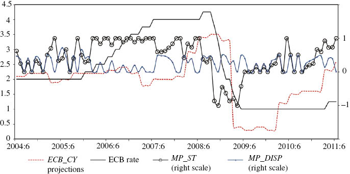
For each month between June 2004 and June 2011, three variables are computed. MP_ST provides the average inclination of all statements during a given month, so the policy stance of Governing council members’ communication. It is comprised between [–1; 1]. MP_INT displays the intensity of the communication so the number of statements times the stance MP_ST, and is used for robustness purposes. Finally, MP_DISP measures the dispersion of statements and is computed as the standard deviation of the stance of all statements during a given month. In a Bayesian updating model, the weight given to the signal (MP_ST) should depend on the precision of the signal. We assume that MP_DISP captures the precision of the signal conveyed in ECB speeches. Figure 1 plots the main ECB communication variables along with the ECB interest rate, while Table 1 provides some descriptive statistics.
Main ECB variables and the KOF index.
Introductory statistics.
| Communication on monetary policy inclination | |||||||
|---|---|---|---|---|---|---|---|
| Tightening | Neutral | Easing | Total | ||||
| 328 | 186 | 75 | 589 | ||||
| 56% | 31% | 13% | 100% | ||||
| Descriptive statistics | |||||||
| Variable | Obs | Mean | Std. dev. | Min | Max | ||
| CF_CY | 85 | 1.90 | 0.80 | 0.27 | 3.61 | ||
| CF_NY | 85 | 1.80 | 0.32 | 1.13 | 2.53 | ||
| ECB_CY | 85 | 1.95 | 0.84 | 0.30 | 3.50 | ||
| ECB_NY | 85 | 1.83 | 0.42 | 1.00 | 2.60 | ||
| ΔECB_CY | 82 | 0.01 | 0.64 | –2.90 | 0.90 | ||
| ΔECB_NY | 82 | 0.00 | 0.33 | –1.20 | 0.50 | ||
| (ECB-CF)_CY | 85 | 0.06 | 0.42 | –0.92 | 2.52 | ||
| (ECB-CF)_NY | 85 | 0.03 | 0.19 | –0.46 | 0.79 | ||
| MP_ST | 85 | 0.44 | 0.53 | –1 | 1 | ||
| ΔMP_ST | 82 | 0.02 | 0.43 | –1.29 | 1 | ||
| MP_INT | 85 | 2.98 | 5.41 | –13.01 | 15.00 | ||
| ECB rate | 85 | 2.33 | 1.15 | 1.00 | 4.25 | ||
| ECB shadow rate | 85 | 2.13 | 1.49 | –0.54 | 4.38 | ||
| Core HICP | 85 | 1.65 | 0.48 | 0.70 | 2.70 | ||
| Output gap | 85 | –0.02 | 1.17 | –2.49 | 2.26 | ||
| Credit growth | 85 | 7.32 | 4.45 | 0.10 | 13.20 | ||
| Oil price | 85 | 24.43 | 37.05 | –54.63 | 86.56 | ||
| VIX | 85 | 20.82 | 10.67 | 10.82 | 62.64 | ||
| Correlation between ECB communication, projections, rate and the KOF index | |||||||
| ECB_CY | ECB_NY | MP_ST | MP_INT | MP_DISP | KOF | ECB rate | |
| ECB_CY | 1 | ||||||
| ECB_NY | 0.74 | 1 | |||||
| MP_ST | 0.18 | 0.46 | 1 | ||||
| MP_INT | 0.14 | 0.41 | 0.91 | 1 | |||
| MP_DISP | 0.07 | –0.09 | –0.15 | –0.15 | 1 | ||
| KOF | 0.56 | 0.71 | 0.58 | 0.54 | –0.07 | 1 | |
| ECB rate | 0.63 | 0.77 | 0.37 | 0.31 | –0.06 | 0.66 | 1 |
| Documenting bias: mean forecast errors | |||||||
| Obs | MFE | Std. dev. | Min | Max | |||
| ECB_CY | 85 | –0.07 | 0.59 | –1.32 | 3.01 | ||
| CF_CY | 85 | –0.12** | 0.26 | –0.94 | 0.75 | ||
| ECB_NY | 79 | –0.22 | 1.07 | –1.42 | 2.31 | ||
| CF_NY | 79 | –0.26 | 1.00 | –1.4 | 2.24 | ||
| Documenting forecasting performance: mean absolute forecast errors | |||||||
| Obs | MAFE | Std. dev. | Min | Max | |||
| ECB_CY | 85 | 0.29*** | 0.52 | 0.01 | 3.01 | ||
| CF_CY | 85 | 0.21*** | 0.20 | 0 | 0.94 | ||
| ECB_NY | 79 | 0.86*** | 0.66 | 0.04 | 2.31 | ||
| CF_NY | 79 | 0.81*** | 0.63 | 0 | 2.24 | ||
**, ***Means forecast errors are significantly different from zero at 5% and 1% levels, respectively. This is estimated with Newey-West procedure (and maximum lag=4) to correct for serial correlation. CY and NY stand for current year and next year forecasts.
Some interesting facts appear from the preceding figure and table. There are much more statements that have a tightening inclination than neutral or easing ones. Fifty-six percentage of the statements made between June 2004 and June 2011 have a hawkish inclination and this makes sense as interest rates were increasing or high for half of the sample period. It is nevertheless interesting to note that the ECB signals much more interest rate hikes than decreases. This is in line with Jansen and De Haan (2009) for the ECB or Hayo and Neuenkirch (2010) for the Federal Reserve who find that these central banks seem cautious about mentioning rate cuts too much. It can also be noted from Figure 1 that ECB projections, the ECB rate and ECB qualitative communication, either MP_ST or KOF (see below), are consistent with each other.
This classification methodology is usually referred to as “content analysis” because of the systematic analysis of the content of a message (Holsti 1969) and it is worth noting that this work is by nature judgmental and subjective. In particular, the choice has been made to focus on forward-looking conventional and unconventional monetary policy announcements with a possible effect on price stability and inflation, and not on policies providing liquidity to money markets and banks. We believe that it is important to differentiate policies aiming at price stability and financial stability following the usual segmentation of monetary policy mandates. Another possible caveat is that Reuters News may have not reported or misinterpreted some statements.
The present index is therefore compared to the KOF monetary policy communicator for the euro area which provides a quantitative measure of the ECB communication with a special focus on forward-looking statements concerning price stability (see Conrad and Lamla (2010) or the KOF website[8] for more details) and is available on the same time span than the present index. It enables to assess the robustness and relevance of the latter. However, the KOF index translates the ECB President’s statement concerning risks to price stability as made during the monthly press conference (and only this specific Governing Council day) as well as ECB projections into a unique common index. In contrast, the index constructed in this paper encompasses all qualitative communication of each month and focuses specifically on speeches and statements in contrast with ECB projections.[9] Table 1 shows the correlation matrix between the KOF index and all indices of this study.[10]
3.2 ECB projections
The ECB/Eurosystem staff macroeconomic projections[11] for the euro area are produced biannually since December 2000, and quarterly since June 2004 with a special emphasis on their disclosure to the public. They are published during the first week of March, June, September and December and are presented as ranges for both the harmonized index for consumer prices (HICP) and real GDP. The ranges are based on twice the mean absolute projection error of historical projection errors to reflect uncertainty. As common for the Federal Open Market Committee (FOMC) at the Federal Reserve forecasts, the midpoint of the range is used to represent ECB projections. Until 2006Q1, the underlying scenarios for interest rates and commodity prices were that these variables remain constant over the projection horizon; since 2006Q2 they are based on market expectations derived from future rates.[12] These projections are published as average annual percentage changes and target current and next years, so are fixed-event projections. They might have seasonal effects as the forecasting horizon decreases quarter after quarter: one might suppose that the effects of ECB inflation projections on private ones are stronger in the beginning of each year and smaller at the end when more information is known on actual variables.[13] Finally, the sample considered here starts in June 2004 when ECB projections became quarterly so as to combine the need for high-frequency data to measure qualitative communication and the relative low-frequency of publication of ECB projections. In addition, we interpolate quarterly ECB projections to monthly frequency by filling the gaps of the 2 months following their disclosure to the public with the value of the last projection published.[14] This assumption seems reasonable as it respects the information structure and corresponds to the information set available to: private agents in the following 2 months of each quarter. However, this assumption introduces a bias against ECB projections which remain constant during 2 months whatever the macroeconomic or policy developments.
3.3 Private forecasts
The private inflation forecasts come from Consensus Economics Inc. The consensus forecasts (CF) is a monthly survey of quantitative predictions of private professional forecasters, with an average of 30 institutional respondents, for about fifteen macroeconomic variables including the overall index for HICP for the euro area (with changing composition), as measured by Eurostat and forecasted by the ECB, and calculated as average annual percentage change for current and next years. Because of its fixed-event nature, the forecasting horizon decreases every month, and we introduce month fixed-effects in our estimations to control for that and propose two robustness tests (see footnote 11). Surveys are collected at the end of the first week or beginning of the second week of each month.
We also consider a financial market-based measure of inflation expectations derived from inflation swaps 5-years 5-years-forward. The instruments are financial market contracts to transfer in 5 years the inflation risk over the 5-years-forward from one counterparty to another. We consider the average of all the working day observations in each month to be consistent with CF data. In general, the advantage of financial market expectations over survey measures of expectations is that they are directly related to payoff decisions, so there is no strategic response bias or no difference between stated and actual beliefs. Although one disadvantage is that financial market expectations do not provide a direct measure of inflation expectations as they may be affected by credit risk, liquidity and inflation risk premia. Swaps tend to be a better market measure for deriving inflation expectations than inflation-indexed bonds because they are generally less sensitive to liquidity and risk premia.
3.4 Other variables
The ECB interest rate considered is the main refinancing operations interest rate. It enables to check whether ECB communication may be a proxy for ECB decisions or whether ECB communication adds some specific information to private inflation expectations’ formation. Indeed, the ECB qualitative communication variable may measure the “procyclical” effect of the speech (e.g. when central bankers say they expect high future inflation, then private inflation expectations should increase) and in the meantime may capture the “countercyclical” effect of the same speech (e.g. when central bankers say they will increase interest rates, private inflation expectations should decrease). With the implementation of non-standard policy measures after 2008, one may argue that the interest rate is not necessarily capturing all aspects of the monetary policy stance. Therefore, we also use the ECB shadow rate estimated by Wu and Xia (2016).
We use various controls for the macroeconomic environment that should in theory impact the private expectations formation. Core the HICP considering all-items excluding energy and unprocessed food, the output gap (the HP-filtered monthly interpolated real GDP), the credit growth rate (to euro area residents other than governments), the oil price growth rate (based on the Brent crude oil spot price) and a proxy for global uncertainty and liquidity risks capturing the financial instability originating in the United States during the 2008–2009 crisis (the VIX index) are included in the empirical model as control variables.[15] These variables, especially the output gap, credit growth and the VIX, also enable to control for the financial turmoil and the great recession that take place during the sample period. The overall sample starts in June 2004, ends in June 2011 and is constituted of 85 monthly observations.
4 Do ECB speeches and projections influence private forecasts?
This section is divided in three parts. First, the econometric approach is described along with the estimation of instruments used to identify the causal effects of ECB projections, qualitative communication and interest rate on private inflation expectations. Second, the linear effects of each ECB variable are examined. Third, their interacted effects are estimated.
4.1 Empirical model
Based on the framework described in Section 2, we estimate the effects of ECB qualitative communication, projections and interest rate on private inflation forecasts beyond the effects of past private inflation forecasts – which explain approximately 85% of the variance of private inflation forecasts – and macroeconomic controls. Alternatively, one can view the expectations formation process as an AR(1) process complemented with the relevant information set used by private agents to predict inflation. Because private inflation forecasts are formed, collected and published at the early beginning of each month and in order to comply with the information timing structure, we assume private inflation forecasts dated t are formed based on the information set dated t–1 (see Figure 2). This is the only information set available to private agents and respecting the data generating process of macroeconomic variables.[16] Based on this information structure constraint, private forecasts at date t are therefore regressed on all variables at date t–1.

Timeline of information structure.
This information set includes variables likely to help predict inflation, in addition to ECB qualitative and quantitative communication and the ECB rate: core HICP, the output gap, credit growth, the oil price and a measure of uncertainty. Core HICP is supposed to affect positively inflation as its underlying fundamental driving force, the output gap similarly through a Phillips curve, credit growth is also supposed to have a positive effect via the quantity theory of money, the oil price is supposed to capture the positive impact of commodity and volatile prices on inflation while the effect of uncertainty may have different effect on inflation expectations: an inflation risk premium would increase inflation, while uncertainty may be associated to recessions and falling inflation. One would also want to include a macroeconomic news variable, but this seems impractical because of the format of private forecasts. Usually the news variable encompassing the information set released between t–1 and t is computed as the difference between the forecast of a given variable (inflation) in t–1 and the actual value of the given variable in t, and this is not possible with CF forecasts as the monthly forecasts are not for the next month horizon. One may nevertheless argue that the news component is small as the ECB qualitative communication variable encompasses all speeches during a given month and all macroeconomic variables are generated at the end of this given month, while private forecasts are formed at the early beginning of the following month. We therefore implicitly assume that price and monetary policy news, which affect expected future inflation (Beechey and Wright 2009), are comprised in t–1 variables and that no news is published between the end of a month and the early beginning of the following month when private agents form their forecasts.
Equation (2) can be rewritten by decomposing the vector Xt–1 in two vectors, one comprising our variables of interest and the other the macroeconomic controls. Because we include a lag of the left-hand side variable in our model, this is equivalent to looking at how inflation expectations change (so having the first difference in inflation expectations as the left-hand side variable) in response to different right-hand side variables, but without an implicit assumption about the inertia coefficient. The estimated equation where yt,h is the private forecast made in t for a given event date h is therefore:
where Πt contains the three policy variables: ECB projections, the ECB qualitative communication (either MP_ST, MP_INT or MP_DISP) and the ECB rate, and Ωt encompasses the macroeconomic controls: core HICP, the output gap, credit growth, the oil price, the proxy for uncertainty and month fixed-effects. The model is estimated with robust standard errors using heteroskedastic and autocorrelation-consistent (HAC) robust variance estimates.[17]
With forward-looking behavior and intertemporal smoothing, random shocks that affect private forecasts are likely to also affect ECB and macro variables, and all those variables are likely to be endogenous to private inflation forecasts (said differently, their correlation with the error term ε is not equal to zero). In order to solve the identification issue, we assume that only our three variables of interest – the vector Πt – are endogenous and that the macro controls are exogenous. The equation (3) is estimated with IV using two-stages-least-squares (2SLS) to identify the causal effects of the three ECB variables.
Another issue arises. The IV estimator requires additional variables that are correlated with these endogenous regressors but not with the error term ε, what Stock, Wright and Yogo (2002) call the “weak identification” problem as instruments are only weakly correlated with the included endogenous variables. Bai and Ng (2010) and Kapetanios and Marcellino (2010) propose to use factor analysis to overcome weak identification in IV estimations as they show that the estimated factors can be more efficient IV than observed variables. Using a principal component analysis, we estimate and generate three factors as linear combinations maximizing the common variance of ECB current- and next-year projections, MP_ST, MP_INT, the ECB rate, the ECB shadow rate, core HICP, the output gap, credit growth, oil prices.[18] We believe this set of variables is relevant because it will generate instruments that encompass the information set of policymakers, their communications and actions, and the most likely economic indicators used in their reaction function. The Kaiser-Meyer-Olkin measure of sampling adequacy provides a simple way to assess the relevance of applying principal component analysis on the selected variables by comparing the partial correlations and correlations between variables and is provided in Table 2 which summarizes the estimation and characteristics of these factors. The first three components capture 87% of the cumulative variance of the underlying series, and we use them as instruments of the vector Πt gathering the three endogenous policy variables.[19]
Factors as instruments.
| Principal components/correlation | Obs=85 | |||
|---|---|---|---|---|
| Rotation: (unrotated=principal) | ρ=0.87 | |||
| Eigenvalue | Difference | Proportion | Cumulative | |
| Comp1 | 5.92 | 3.98 | 0.59 | 0.59 |
| Comp2 | 1.94 | 1.16 | 0.19 | 0.79 |
| Comp3 | 0.79 | 0.36 | 0.08 | 0.87 |
| Principal components (eigenvectors) | ||||
| Variable | Comp1 | Comp2 | Comp3 | Unexplained |
| ECB_CY | 0.30 | –0.25 | 0.34 | 0.24 |
| ECB_NY | 0.36 | –0.05 | 0.11 | 0.20 |
| MP_ST | 0.25 | 0.51 | –0.30 | 0.05 |
| MP_INT | 0.23 | 0.53 | –0.26 | 0.08 |
| ECB rate | 0.37 | –0.20 | –0.19 | 0.07 |
| Shadow | 0.39 | –0.10 | –0.14 | 0.05 |
| Core | 0.31 | –0.32 | 0.17 | 0.20 |
| Output gap | 0.34 | 0.17 | 0.21 | 0.24 |
| Credit growth | 0.36 | –0.18 | –0.32 | 0.10 |
| Oil | 0.16 | 0.42 | 0.70 | 0.12 |
| Kaiser-Meyer-Olkin measure of sampling adequacy: 0.81 | ||||
| Predictive power of factors vs. an AR(1) model | ||||
| Adj. R2 | ECB_CY | ECB_NY | MP_ST | ECB rate |
| Factors | 0.75 | 0.79 | 0.94 | 0.93 |
| AR(1) model | 0.81 | 0.42 | 0.61 | 0.98 |
Tests of weak identification are reported in Table 2 and at the bottom of Tables 3–8.[20] First, we assess the predictive power for the endogenous regressors of our three instruments compared to a simple AR(1) model (the use of lags as instruments being the benchmark in the macroeconomic literature) and provide the corresponding adjusted R2 in Table 2. Second, the Cragg-Donald Wald test statistic assesses whether the excluded instruments are correlated with the endogenous regressors. A rejection of the null should be treated with caution however, because weak instrument problems may still be present. Third, the Anderson canonical correlations LM statistic informs whether the equation is identified – that the excluded instruments are correlated with the endogenous regressors. Under the null, the statistic is distributed as χ2 with 1 degree of freedom here. A rejection of the null indicates that the model is identified. All tests confirm that the instrument set is relevant for identifying the causal effect of the three variables of interest.[21]
IV 2SLS estimation of the effects of ECB action and communications on private current-year inflation forecasts.
| Dependent variable: CF current-year inflation forecasts | ||||||||||||||||
|---|---|---|---|---|---|---|---|---|---|---|---|---|---|---|---|---|
| (1) Baseline | (2) Shadow | (3) w/o Qual. | (4) w/o Quant. | (5) LIML | (6) MP_INT | (7) ΔComVar | (8) (ECB-CF) | (9) Post2006 | (10) Semester | (11) ECB_NY | (12) Quarterly | (13) MP_DISP | (14) PR_ST | (15) NPR_ST | (16) MP_ST2 | |
| ECB_CY | 0.256** | 0.253** | 0.263** | . | 0.256** | 0.252** | 0.199 | 0.253** | 0.261*** | 0.689** | 0.587*** | 0.234** | 0.257** | 0.257** | 0.257** | |
| [0.11] | [0.10] | [0.11] | [0.11] | [0.11] | [0.17] | [0.10] | [0.10] | [0.34] | [0.08] | [0.09] | [0.11] | [0.11] | [0.11] | |||
| MP_ST | –0.069 | –0.056 | . | –0.124 | –0.069 | –0.006 | –0.169 | –0.072 | –0.209 | –0.134 | –0.181 | 0.026 | –0.122 | –0.074 | –0.07 | –0.069 |
| [0.13] | [0.10] | [0.13] | [0.13] | [0.01] | [0.19] | [0.13] | [0.18] | [0.13] | [0.11] | [0.02] | [0.15] | [0.14] | [0.13] | [0.13] | ||
| ECB rate | 0.06 | 0.057 | 0.063 | –0.034 | 0.06 | 0.049 | –0.221 | 0.059 | 0.082 | 0.079 | –0.099 | –0.051** | 0.039 | 0.06 | 0.062 | 0.057 |
| [0.15] | [0.14] | [0.16] | [0.11] | [0.15] | [0.14] | [0.11] | [0.15] | [0.15] | [0.14] | [0.08] | [0.02] | [0.14] | [0.15] | [0.16] | [0.15] | |
| CF_CY | 0.501*** | 0.488*** | 0.496*** | 0.715*** | 0.501*** | 0.503*** | 0.583*** | 0.756*** | 0.490*** | 0.633*** | 0.533*** | 0.398*** | 0.530*** | 0.497*** | 0.496*** | 0.498*** |
| [0.09] | [0.11] | [0.09] | [0.08] | [0.09] | [0.09] | [0.16] | [0.07] | [0.09] | [0.14] | [0.12] | [0.08] | [0.07] | [0.09] | [0.09] | [0.09] | |
| Core HICP | –0.137 | –0.127 | –0.109 | –0.071 | –0.137 | –0.117 | 0.137 | –0.148 | –0.169 | –0.177 | 0.065 | 0.100*** | –0.129 | –0.129 | –0.145 | –0.133 |
| [0.14] | [0.11] | [0.11] | [0.09] | [0.14] | [0.12] | [0.14] | [0.14] | [0.26] | [0.13] | [0.10] | [0.02] | [0.13] | [0.13] | [0.15] | [0.13] | |
| Output gap | 0.132*** | 0.129** | 0.113** | 0.148*** | 0.132*** | 0.132*** | 0.142** | 0.134*** | 0.153** | 0.118 | 0.112*** | 0.019 | 0.144*** | 0.132*** | 0.133*** | 0.132*** |
| [0.05] | [0.05] | [0.05] | [0.05] | [0.05] | [0.05] | [0.06] | [0.05] | [0.07] | [0.06] | [0.04] | [0.01] | [0.04] | [0.05] | [0.05] | [0.05] | |
| Credit growth | –0.002 | –0.004 | –0.005 | 0.024 | –0.002 | –0.001 | 0.060** | 0 | –0.002 | –0.001 | 0.008 | 0.001 | 0.002 | –0.002 | –0.001 | –0.001 |
| [0.02] | [0.03] | [0.03] | [0.02] | [0.02] | [0.02] | [0.03] | [0.02] | [0.02] | [0.02] | [0.02] | [0.01] | [0.02] | [0.02] | [0.02] | [0.02] | |
| Oil price | 0.005*** | 0.005*** | 0.005*** | 0.004*** | 0.005*** | 0.005*** | 0.003*** | 0.005*** | 0.005*** | 0.004*** | 0.004*** | 0.000 | 0.005*** | 0.005*** | 0.005*** | 0.005*** |
| [0.00] | [0.00] | [0.00] | [0.00] | [0.00] | [0.00] | [0.00] | [0.00] | [0.00] | [0.00] | [0.00] | [0.00] | [0.00] | [0.00] | [0.00] | [0.00] | |
| VIX | –0.002 | –0.001 | –0.001 | –0.001 | –0.002 | –0.002 | 0.002 | –0.002 | –0.006 | –0.003 | –0.002 | 0.000 | –0.003 | –0.003 | –0.002 | –0.002 |
| [0.00] | [0.00] | [0.00] | [0.00] | [0.00] | [0.00] | [0.00] | [0.00] | [0.00] | [0.00] | [0.00] | [0.00] | [0.00] | [0.00] | [0.00] | [0.00] | |
| ECB_CY_sem1 | . | . | . | . | . | . | . | . | . | 0.220** | . | . | . | . | . | . |
| [0.09] | ||||||||||||||||
| ECB_CY_sem2 | . | . | . | . | . | . | . | . | . | 0.104 | . | . | . | . | . | . |
| [0.13] | ||||||||||||||||
| MP_DISP | . | . | . | . | . | . | . | . | . | . | . | . | –0.187 | . | . | . |
| [0.15] | ||||||||||||||||
| Constant | 0.328** | 0.337** | 0.239 | 0.351 | 0.328** | 0.304 | 0.349 | 0.337** | 0.478** | 0.427*** | –0.501 | –0.051 | 0.411*** | 0.333** | 0.331 | 0.328** |
| [0.17] | [0.15] | [0.23] | [0.18] | [0.17] | [0.17] | [0.20] | [0.16] | [0.19] | [0.17] | [0.49] | [0.04] | [0.15] | [0.17] | [0.17] | [0.17] | |
| Nb. of obs | 84 | 84 | 84 | 84 | 84 | 84 | 81 | 83 | 62 | 83 | 84 | 26 | 84 | 84 | 84 | 84 |
| R2 | 0.93 | 0.93 | 0.92 | 0.93 | 0.93 | 0.93 | 0.91 | 0.93 | 0.93 | 0.93 | 0.95 | 1.00 | 0.93 | 0.93 | 0.92 | 0.93 |
| Cragg-Donald Wald stat | 139.44 | 157.01 | 167.85 | 296.03 | 139.44 | 131.05 | 40.74 | 142.19 | 116.88 | 26.23 | 57.42 | 11.47 | 143.95 | 57.01 | 97.90 | 134.03 |
| χ2(1) p-value | 0.00 | 0.00 | 0.00 | 0.00 | 0.00 | 0.00 | 0.00 | 0.00 | 0.00 | 0.00 | 0.00 | 0.01 | 0.00 | 0.00 | 0.00 | 0.00 |
| Anderson LM stat | 82.18 | 88.54 | 92.23 | 126.79 | 82.18 | 78.96 | 33.00 | 82.84 | 65.69 | 22.79 | 43.75 | 9.50 | 83.86 | 43.51 | 64.90 | 80.12 |
| χ2(1) p-value | 0.00 | 0.00 | 0.00 | 0.00 | 0.00 | 0.00 | 0.00 | 0.00 | 0.00 | 0.00 | 0.00 | 0.02 | 0.00 | 0.00 | 0.00 | 0.00 |
**, ***Means coefficients are significant at 5% and 1%, respectively. Robust standard errors in brackets. Heteroskedastic and autocorrelation-consistent (HAC) robust variance estimated with bandwich equal to 12. The dependent variable is private inflation forecasts at date t, while all regressors are from date t–1. The equation also includes month fixed effects. Instruments are the t–1 first 3 components of a principal component analysis of ECB_CY, ECB_NY, MP_ST, MP_INT, ECB rate, ECB shadow rate, core HICP, output gap, credit growth, oil prices. Our main variables of interest – the three policy variables – are considered endogenous and instrumented. The equation is therefore exactly identified. We provide the Cragg-Donald Wald underidentification test and Anderson canonical correlations underidentification test statistics and p-values. In column 2, the ECB rate is replaced by the ECB shadow rate estimated by Wu and Xia (2016). In column 5, the GMM generalization of the LIML estimator to the case of possibly heteroskedastic and autocorrelated disturbances – the continuously updated GMM estimator or CUE – is used. In column 6, the ECB qualitative communication variable MP_ST is replaced by MP_INT. In columns 7 and 8, it is the ECB quantitative communication – the ECB projections – which is replaced by the quarter-over-quarter difference in ECB projections and the difference between ECB projections and CF forecasts, respectively. In column 9, the sample starts in 2006m4. In column 10, the ECB projections are split into two variables for ECB projections published during the first semester and the second one. In column 11, ECB next year projections replace the ECB current year ones. In column 12, the frequency is quarterly. In column 13, the dispersion of the ECB qualitative communication is added. MP_ST is replaced by PR_ST and NPR_ST, communication indices for the President and other members of the Governing Council, in columns 14 and 15, respectively. In column 16, the monthly communication index is computed with only the communications happening after the policy decision.
IV 2SLS estimation of the effects of ECB action and communications on private next-year forecasts.
| Dependent variable: CF next-year inflation forecasts | ||||||||||||||||
|---|---|---|---|---|---|---|---|---|---|---|---|---|---|---|---|---|
| (1) Baseline | (2) Shadow | (3) w/o Qual. | (4) w/o Quant. | (5) LIML | (6) MP_INT | (7) ΔComVar | (8) (ECB-CF) | (9) Post2006 | (10) Semester | (11) ECB_CY | (12) Quarterly | (13) MP_DISP | (14) PR_ST | (15) NPR_ST | (16) MP_ST2 | |
| ECB_NY | 0.037 | 0.096 | 0.058 | . | 0.037 | 0.045 | –0.156 | 0.078 | 0.248 | . | 0.009 | 0.213 | 0.048 | 0.023 | 0.053 | 0.039 |
| [0.07] | [0.07] | [0.07] | [0.07] | [0.07] | [0.10] | [0.08] | [0.16] | [0.02] | [0.13] | [0.09] | [0.08] | [0.08] | [0.07] | |||
| MP_ST | 0.076 | 0.049 | . | 0.078 | 0.076 | 0.006 | 0.052** | 0.068 | 0.002 | 0.03 | 0.081 | 0.078* | 0.091 | 0.082 | 0.077 | 0.076 |
| [0.05] | [0.05] | [0.05] | [0.05] | [0.00] | [0.03] | [0.05] | [0.07] | [0.04] | [0.05] | [0.04] | [0.06] | [0.05] | [0.05] | [0.05] | ||
| ECB rate | –0.085*** | –0.090*** | –0.085** | –0.085*** | –0.085*** | –0.075*** | –0.055** | –0.091** | –0.095** | –0.051 | –0.079** | –0.069*** | –0.079** | –0.086*** | –0.088** | –0.082*** |
| [0.03] | [0.03] | [0.03] | [0.03] | [0.03] | [0.03] | [0.03] | [0.04] | [0.04] | [0.04] | [0.03] | [0.02] | [0.03] | [0.03] | [0.04] | [0.03] | |
| CF_NY | 0.622*** | 0.617*** | 0.604*** | 0.655*** | 0.622*** | 0.623*** | 0.700*** | 0.662*** | 0.409*** | 0.893*** | 0.638*** | 0.565*** | 0.608*** | 0.652*** | 0.612*** | 0.623*** |
| [0.09] | [0.09] | [0.11] | [0.06] | [0.09] | [0.09] | [0.06] | [0.06] | [0.15] | [0.18] | [0.07] | [0.11] | [0.11] | [0.10] | [0.10] | [0.09] | |
| Core HICP | 0.045 | 0.046 | 0.013 | 0.042 | 0.045 | 0.026 | –0.021 | 0.054 | 0.198 | 0.012 | 0.036 | 0.140*** | 0.044 | 0.036 | 0.057 | 0.041 |
| [0.06] | [0.06] | [0.05] | [0.06] | [0.06] | [0.05] | [0.03] | [0.07] | [0.13] | [0.06] | [0.05] | [0.04] | [0.06] | [0.06] | [0.07] | [0.06] | |
| Output gap | 0.038** | 0.043** | 0.055*** | 0.041*** | 0.038** | 0.037** | 0.059*** | 0.038 | –0.004 | 0.024 | 0.039** | 0.005 | 0.033 | 0.038** | 0.036** | 0.037** |
| [0.02] | [0.02] | [0.02] | [0.01] | [0.02] | [0.02] | [0.01] | [0.02] | [0.04] | [0.02] | [0.02] | [0.01] | [0.02] | [0.02] | [0.02] | [0.02] | |
| Credit growth | 0.024*** | 0.028*** | 0.027*** | 0.025*** | 0.024*** | 0.024*** | 0.021*** | 0.025*** | 0.018** | 0.014 | 0.024*** | 0.010*** | 0.023*** | 0.025*** | 0.023*** | 0.024*** |
| [0.01] | [0.01] | [0.01] | [0.01] | [0.01] | [0.01] | [0.01] | [0.01] | [0.01] | [0.01] | [0.01] | [0.00] | [0.01] | [0.01] | [0.01] | [0.01] | |
| Oil price | 0.001*** | 0.001*** | 0.001** | 0.001*** | 0.001*** | 0.001*** | 0.001*** | 0.001** | 0.001*** | 0.001** | 0.001*** | 0 | 0.001** | 0.001*** | 0.001** | 0.001*** |
| [0.00] | [0.00] | [0.00] | [0.00] | [0.00] | [0.00] | [0.00] | [0.00] | [0.00] | [0.00] | [0.00] | [0.00] | [0.00] | [0.00] | [0.00] | [0.00] | |
| VIX | 0.000 | –0.003 | –0.002 | 0.000 | 0.000 | 0.000 | –0.002 | 0.000 | –0.007** | 0.000 | 0.000 | –0.005*** | 0.000 | 0.001 | 0.000 | 0.000 |
| [0.00] | [0.00] | [0.00] | [0.00] | [0.00] | [0.00] | [0.00] | [0.00] | [0.00] | [0.00] | [0.00] | [0.00] | [0.00] | [0.00] | [0.00] | [0.00] | |
| ECB_NY_sem1 | . | . | . | . | . | . | . | . | . | 0.069 | . | . | . | . | . | . |
| [0.06] | ||||||||||||||||
| ECB_NY_sem2 | . | . | . | . | . | . | . | . | . | –0.169 | . | . | . | . | . | . |
| [0.14] | ||||||||||||||||
| MP_DISP | . | . | . | . | . | . | . | . | . | . | . | . | 0.057 | . | . | . |
| [0.08] | ||||||||||||||||
| Constant | 0.503*** | 0.427*** | 0.595*** | 0.510*** | 0.503*** | 0.517*** | 0.541*** | 0.504*** | 0.517*** | 0.483*** | 0.528*** | 0.328*** | 0.480*** | 0.478*** | 0.495*** | 0.499*** |
| [0.11] | [0.10] | [0.14] | [0.11] | [0.11] | [0.10] | [0.14] | [0.11] | [0.09] | [0.10] | [0.12] | [0.03] | [0.12] | [0.12] | [0.11] | [0.11] | |
| Nb. of obs | 84 | 84 | 84 | 84 | 84 | 84 | 81 | 83 | 62 | 83 | 84 | 26 | 84 | 84 | 84 | 84 |
| R2 | 0.93 | 0.92 | 0.92 | 0.93 | 0.93 | 0.93 | 0.94 | 0.92 | 0.92 | 0.93 | 0.93 | 0.98 | 0.93 | 0.92 | 0.92 | 0.93 |
| Cragg-Donald Wald stat | 45.27 | 42.36 | 48.09 | 296.01 | 45.27 | 46.79 | 52.10 | 46.96 | 28.81 | 23.37 | 169.51 | 29.28 | 47.13 | 39.35 | 47.93 | 45.37 |
| χ2(1) p-value | 0.00 | 0.00 | 0.00 | 0.00 | 0.00 | 0.00 | 0.00 | 0.00 | 0.00 | 0.00 | 0.00 | 0.00 | 0.00 | 0.00 | 0.00 | 0.00 |
| Anderson LM stat | 36.21 | 34.30 | 38.02 | 126.79 | 36.21 | 37.19 | 40.23 | 37.22 | 23.66 | 20.59 | 92.78 | 19.61 | 37.41 | 32.28 | 37.92 | 36.27 |
| χ2(1) p-value | 0.00 | 0.00 | 0.00 | 0.00 | 0.00 | 0.00 | 0.00 | 0.00 | 0.00 | 0.00 | 0.00 | 0.00 | 0.00 | 0.00 | 0.00 | 0.00 |
**, ***Means coefficients are significant at 5% and 1%, respectively. Robust standard errors in brackets. Heteroskedastic and autocorrelation-consistent (HAC) robust variance estimated with bandwich equal to 12. The dependent variable is private inflation forecasts at date t, while all regressors are from date t–1. The equation also includes month fixed effects. Instruments are the t–1 first 3 components of a principal component analysis of ECB_CY, ECB_NY, MP_ST, MP_INT, ECB rate, ECB shadow rate, core HICP, output gap, credit growth, oil prices. Our main variables of interest – the three policy variables – are considered endogenous and instrumented. The equation is therefore exactly identified. We provide the Cragg-Donald Wald underidentification test and Anderson canonical correlations underidentification test statistics and p-values. In column 2, the ECB rate is replaced by the ECB shadow rate estimated by Wu and Xia (2016). In column 5, the GMM generalization of the LIML estimator to the case of possibly heteroskedastic and autocorrelated disturbances – the continuously updated GMM estimator or CUE – is used. In column 6, the ECB qualitative communication variable MP_ST is replaced by MP_INT. In columns 7 and 8, it is the ECB quantitative communication – the ECB projections – which is replaced by the quarter-over-quarter difference in ECB projections and the difference between ECB projections and CF forecasts, respectively. In column 9, the sample starts in 2006m4. In column 10, the ECB projections are split into two variables for ECB projections published during the first semester and the second one. In column 11, ECB current-year projections replace the ECB next-year ones. In column 12, the frequency is quarterly. In column 13, the dispersion of the ECB qualitative communication is added. MP_ST is replaced by PR_ST and NPR_ST, communication indices for the President and other members of the Governing Council, in columns 14 and 15, respectively. In column 16, the monthly communication index is computed with only the communications happening after the policy decision.
IV 2SLS estimation of the effects of ECB action and communications on private 1-year ahead forecasts.
| Dependent variable: CF 1-year ahead inflation forecasts | ||||||||||||||
|---|---|---|---|---|---|---|---|---|---|---|---|---|---|---|
| (1) Baseline | (2) Shadow | (3) w/o Qual. | (4) w/o Quant. | (5) LIML | (6) MP_INT | (7) ΔComVar | (8) (ECB-CF) | (9) Post2006 | (10) Quarterly | (11) MP_DISP | (12) PR_ST | (13) NPR_ST | (14) MP_ST2 | |
| ECB_1Y | 0.015 | 0.029 | 0.000 | . | –0.012 | 0.026 | –0.008 | 0.036 | 0.012 | 0.518*** | 0.015 | 0.001 | 0.002 | 0.000 |
| [0.02] | [0.02] | [0.02] | [0.04] | [0.02] | [0.01] | [0.02] | [0.02] | [0.09] | [0.02] | [0.02] | [0.02] | [0.02] | ||
| MP_ST | 0.05 | –0.005 | . | 0.05 | 0.067 | 0.005 | 0.086*** | 0.051 | 0.006 | 0.035 | 0.045 | 0.049 | 0.060** | 0.048 |
| [0.03] | [0.05] | [0.03] | [0.04] | [0.00] | [0.02] | [0.03] | [0.06] | [0.03] | [0.03] | [0.03] | [0.02] | [0.03] | ||
| ECB rate | –0.166*** | –0.192*** | –0.146*** | –0.148*** | –0.185*** | –0.170*** | –0.135*** | –0.195*** | –0.176*** | –0.109*** | –0.170*** | –0.146*** | –0.149*** | –0.146*** |
| [0.03] | [0.06] | [0.03] | [0.03] | [0.03] | [0.03] | [0.02] | [0.03] | [0.04] | [0.02] | [0.03] | [0.03] | [0.02] | [0.03] | |
| CF_1Y | 0.641*** | 0.717*** | 0.671*** | 0.668*** | 0.689*** | 0.625*** | 0.701*** | 0.639*** | 0.645*** | 0.372*** | 0.641*** | 0.675*** | 0.670*** | 0.670*** |
| [0.04] | [0.04] | [0.04] | [0.03] | [0.06] | [0.03] | [0.04] | [0.04] | [0.03] | [0.08] | [0.04] | [0.03] | [0.03] | [0.03] | |
| Core HICP | 0.055 | 0.030 | 0.026 | 0.051 | 0.079** | 0.043 | 0.04 | 0.062 | 0.147*** | 0.141*** | 0.056 | 0.041 | 0.064 | 0.047 |
| [0.04] | [0.03] | [0.04] | [0.04] | [0.04] | [0.04] | [0.04] | [0.05] | [0.04] | [0.04] | [0.04] | [0.04] | [0.04] | [0.04] | |
| Output gap | 0.134*** | 0.151*** | 0.136*** | 0.124*** | 0.127*** | 0.139*** | 0.127*** | 0.148*** | 0.111*** | 0.051*** | 0.136*** | 0.124*** | 0.121*** | 0.124*** |
| [0.02] | [0.03] | [0.01] | [0.02] | [0.02] | [0.02] | [0.02] | [0.02] | [0.03] | [0.01] | [0.02] | [0.02] | [0.02] | [0.02] | |
| Credit growth | 0.037*** | 0.050*** | 0.035*** | 0.033*** | 0.039*** | 0.039*** | 0.031*** | 0.042*** | 0.035*** | 0.013** | 0.037*** | 0.033*** | 0.031*** | 0.032*** |
| [0.01] | [0.02] | [0.01] | [0.01] | [0.01] | [0.01] | [0.01] | [0.01] | [0.01] | [0.01] | [0.01] | [0.01] | [0.01] | [0.01] | |
| Oil price | 0.002*** | 0.002*** | 0.002*** | 0.002*** | 0.001*** | 0.002*** | 0.002*** | 0.002*** | 0.002*** | 0.000 | 0.002*** | 0.002*** | 0.002*** | 0.002*** |
| [0.00] | [0.00] | [0.00] | [0.00] | [0.00] | [0.00] | [0.00] | [0.00] | [0.00] | [0.00] | [0.00] | [0.00] | [0.00] | [0.00] | |
| VIX | –0.002 | –0.007*** | –0.003** | –0.002 | 0.000 | –0.002 | –0.002 | –0.001 | –0.005*** | –0.003** | –0.002 | –0.002 | –0.002 | –0.002 |
| [0.00] | [0.00] | [0.00] | [0.00] | [0.00] | [0.00] | [0.00] | [0.00] | [0.00] | [0.00] | [0.00] | [0.00] | [0.00] | [0.00] | |
| MP_DISP | . | . | . | . | . | . | . | . | . | . | –0.025 | . | . | . |
| [0.03] | ||||||||||||||
| Constant | 0.602*** | 0.523*** | 0.639*** | 0.577*** | 0.582*** | 0.631*** | 0.541*** | 0.636*** | 0.591*** | 0.157*** | 0.612*** | 0.573*** | 0.560*** | 0.578*** |
| [0.10] | [0.10] | [0.06] | [0.09] | [0.08] | [0.09] | [0.08] | [0.10] | [0.13] | [0.04] | [0.09] | [0.09] | [0.07] | [0.08] | |
| Nb. of obs | 83 | 83 | 83 | 83 | 83 | 83 | 80 | 83 | 62 | 26 | 83 | 83 | 83 | 83 |
| R2 | 0.99 | 0.99 | 0.99 | 0.99 | 0.99 | 0.99 | 0.99 | 0.99 | 0.99 | 1.00 | 0.99 | 0.99 | 0.99 | 0.99 |
| Cragg-Donald Wald stat | 29.35 | 15.83 | 950.35 | 384.61 | 29.35 | 27.93 | 136.99 | 91.44 | 27.31 | 25.45 | 29.13 | 75.25 | 127.37 | 305.80 |
| χ2(1) p-value | 0.00 | 0.00 | 0.00 | 0.00 | 0.00 | 0.00 | 0.00 | 0.00 | 0.00 | 0.00 | 0.00 | 0.00 | 0.00 | 0.00 |
| Anderson LM stat | 25.13 | 14.48 | 209.30 | 143.49 | 25.13 | 24.07 | 79.83 | 61.65 | 22.63 | 17.75 | 24.97 | 53.57 | 77.19 | 128.17 |
| χ2(1) p-value | 0.00 | 0.00 | 0.00 | 0.00 | 0.00 | 0.00 | 0.00 | 0.00 | 0.00 | 0.00 | 0.00 | 0.00 | 0.00 | 0.00 |
**, ***Means coefficients are significant at 5% and 1%, respectively. Robust standard errors in brackets. Heteroskedastic and autocorrelation-consistent (HAC) robust variance estimated with bandwich equal to 12. ECB_1Y are constructed as in Dovern, Fritsche, and Slacalek (2012). The dependent variable is private inflation forecasts at date t, while all regressors are from date t–1. The equation also includes month fixed effects. Instruments are the t–1 first 3 components of a principal component analysis of ECB_1Y, MP_ST, MP_INT, ECB rate, ECB shadow rate, core HICP, output gap, credit growth, oil prices. Our main variables of interest – the three policy variables – are considered endogenous and instrumented. The equation is therefore exactly identified. We provide the Cragg-Donald Wald underidentification test and Anderson canonical correlations underidentification test statistics and p-values. In column 2, the ECB rate is replaced by the ECB shadow rate estimated by Wu and Xia (2016). In column 5, the GMM generalization of the LIML estimator to the case of possibly heteroskedastic and autocorrelated disturbances -the continuously updated GMM estimator or CUE- is used. In column 6, the ECB qualitative communication variable MP_ST is replaced by MP_INT. In columns 7 and 8, it is the ECB quantitative communication – the ECB projections – which is replaced by the quarter-over-quarter difference in ECB projections and the difference between ECB projections and CF forecasts, respectively. In column 9, the sample starts in 2006m4. In column 10, the frequency is quarterly. In column 11, the dispersion of the ECB qualitative communication is added. MP_ST is replaced by PR_ST and NPR_ST, communication indices for the President and other members of the Governing Council, in columns 12 and 13, respectively. In column 14, the monthly communication index is computed with only the communications happening after the policy decision.
IV 2SLS estimation of the effects of ECB action and communications on 5-year 5-year-forward inflation swaps.
| Dependent variable: 5-year 5-year-forward inflation swaps | ||||||||||||||
|---|---|---|---|---|---|---|---|---|---|---|---|---|---|---|
| (1) Baseline | (2) Shadow | (3) w/o Qual. | (4) w/o Quant. | (5) LIML | (6) MP_INT | (7) ΔComVar | (8) (ECB-CF) | (9) Post2006 | (10) ECB_CY | (11) MP_DISP | (12) PR_ST | (13) NPR_ST | (14) MP_ST2 | |
| ECB_NY | –0.128** | –0.115 | –0.143** | . | –0.128** | –0.127 | –0.008 | –0.118** | –0.158** | –0.041** | –0.130** | –0.133** | –0.131** | –0.128** |
| [0.06] | [0.07] | [0.07] | [0.06] | [0.07] | [0.04] | [0.06] | [0.07] | [0.02] | [0.06] | [0.06] | [0.06] | [0.06] | ||
| MP_ST | –0.041 | –0.044 | . | –0.070** | –0.041 | –0.004 | –0.050** | –0.051 | –0.063 | –0.067** | –0.059 | –0.042 | –0.045 | –0.043 |
| [0.04] | [0.04] | [0.03] | [0.04] | [0.00] | [0.02] | [0.03] | [0.07] | [0.03] | [0.04] | [0.04] | [0.04] | [0.04] | ||
| ECB rate | –0.051** | –0.047** | –0.043** | –0.064*** | –0.051** | –0.061** | –0.099*** | –0.056*** | –0.062** | –0.082*** | –0.057*** | –0.049** | –0.050** | –0.054** |
| [0.02] | [0.02] | [0.02] | [0.02] | [0.02] | [0.03] | [0.03] | [0.02] | [0.03] | [0.02] | [0.02] | [0.02] | [0.02] | [0.02] | |
| SWAP_5Y5Y | 0.906*** | 0.862*** | 0.870*** | 0.990*** | 0.906*** | 0.927*** | 1.031*** | 0.802*** | 0.840*** | 0.927*** | 0.906*** | 0.899*** | 0.914*** | 0.912*** |
| [0.08] | [0.07] | [0.07] | [0.06] | [0.08] | [0.09] | [0.07] | [0.10] | [0.08] | [0.06] | [0.07] | [0.07] | [0.08] | [0.08] | |
| Core HICP | –0.022 | –0.016 | 0.002 | –0.037** | –0.022 | –0.017 | –0.004 | –0.033 | 0.000 | 0.007 | –0.02 | –0.016 | –0.032 | –0.022 |
| [0.02] | [0.02] | [0.02] | [0.02] | [0.02] | [0.01] | [0.02] | [0.02] | [0.05] | [0.02] | [0.02] | [0.02] | [0.02] | [0.02] | |
| Output gap | 0.056*** | 0.054*** | 0.043*** | 0.051*** | 0.056*** | 0.059*** | 0.044*** | 0.059*** | 0.048 | 0.056*** | 0.061*** | 0.055*** | 0.058*** | 0.057*** |
| [0.02] | [0.02] | [0.01] | [0.01] | [0.02] | [0.02] | [0.01] | [0.01] | [0.03] | [0.01] | [0.02] | [0.02] | [0.02] | [0.02] | |
| Credit growth | 0.020*** | 0.021*** | 0.017*** | 0.017*** | 0.020*** | 0.021*** | 0.020*** | 0.021*** | 0.024*** | 0.022*** | 0.021*** | 0.019*** | 0.021*** | 0.020*** |
| [0.01] | [0.01] | [0.00] | [0.01] | [0.01] | [0.01] | [0.01] | [0.01] | [0.01] | [0.01] | [0.01] | [0.01] | [0.01] | [0.01] | |
| Oil price | 0.000 | 0.000 | 0.000 | –0.001*** | 0.000 | 0.000 | –0.001*** | 0.000 | 0.000 | –0.000** | 0.000 | 0.000 | 0.000 | 0.000 |
| [0.00] | [0.00] | [0.00] | [0.00] | [0.00] | [0.00] | [0.00] | [0.00] | [0.00] | [0.00] | [0.00] | [0.00] | [0.00] | [0.00] | |
| VIX | 0.001 | 0.000 | 0.001 | –0.001 | 0.001 | 0.000 | 0.000 | 0.000 | 0.000 | 0.000 | 0.000 | 0.000 | 0.000 | 0.000 |
| [0.00] | [0.00] | [0.00] | [0.00] | [0.00] | [0.00] | [0.00] | [0.00] | [0.00] | [0.00] | [0.00] | [0.00] | [0.00] | [0.00] | |
| MP_DISP | . | . | . | . | . | . | . | . | . | . | –0.068 | . | . | |
| [0.05] | ||||||||||||||
| Constant | 0.455** | 0.511** | 0.490** | 0.135 | 0.455** | 0.403 | –0.001 | 0.428** | 0.637*** | 0.267** | 0.488** | 0.475** | 0.445** | 0.445** |
| [0.21] | [0.21] | [0.21] | [0.13] | [0.21] | [0.23] | [0.14] | [0.18] | [0.20] | [0.13] | [0.21] | [0.20] | [0.21] | [0.21] | |
| Nb. of obs | 84 | 83 | 84 | 84 | 84 | 84 | 81 | 83 | 62 | 84 | 84 | 84 | 84 | 84 |
| R2 | 0.82 | 0.83 | 0.81 | 0.83 | 0.82 | 0.81 | 0.81 | 0.82 | 0.81 | 0.84 | 0.83 | 0.82 | 0.81 | 0.82 |
| Cragg-Donald Wald stat | 76.45 | 73.30 | 107.13 | 240.86 | 76.45 | 71.88 | 51.74 | 85.79 | 53.50 | 195.40 | 82.10 | 47.66 | 61.93 | 70.82 |
| χ2(1)p-value | 0.00 | 0.00 | 0.00 | 0.00 | 0.00 | 0.00 | 0.00 | 0.00 | 0.00 | 0.00 | 0.00 | 0.00 | 0.00 | 0.00 |
| Anderson LM stat | 54.36 | 52.54 | 69.06 | 113.62 | 54.36 | 51.94 | 40.01 | 58.91 | 38.57 | 100.95 | 57.27 | 37.75 | 46.39 | 51.36 |
| χ2(1) p-value | 0.00 | 0.00 | 0.00 | 0.00 | 0.00 | 0.00 | 0.00 | 0.00 | 0.00 | 0.00 | 0.00 | 0.00 | 0.00 | 0.00 |
**, ***Means coefficients are significant at 5% and 1%, respectively. Robust standard errors in brackets. Heteroskedastic and autocorrelation-consistent (HAC) robust variance estimated with bandwich equal to 12. The dependent variable is private inflation forecasts at date t, while all regressors are from date t–1. The equation also includes month fixed effects. Instruments are the t–1 first 3 components of a principal component analysis of ECB_1Y, MP_ST, MP_INT, ECB rate, ECB shadow rate, core HICP, output gap, credit growth, oil prices. Our main variables of interest – the three policy variables – are considered endogenous and instrumented. The equation is therefore exactly identified. We provide the Cragg-Donald Wald underidentification test and Anderson canonical correlations underidentification test statistics and p-values. In column 2, the ECB rate is replaced by the ECB shadow rate estimated by Wu and Xia (2016). In column 5, the GMM generalization of the LIML estimator to the case of possibly heteroskedastic and autocorrelated disturbances – the continuously updated GMM estimator or CUE – is used. In column 6, the ECB qualitative communication variable MP_ST is replaced by MP_INT. In columns 7 and 8, it is the ECB quantitative communication – the ECB projections – which is replaced by the quarter-over-quarter difference in ECB projections and the difference between ECB projections and CF forecasts, respectively. In column 9, the sample starts in 2006m4. In column 10, ECB current-year projections replace the ECB next-year ones. In column 11, the dispersion of the ECB qualitative communication is added. MP_ST is replaced by PR_ST and NPR_ST, communication indices for the President and other members of the Governing Council, in columns 12 and 13, respectively. In column 14, the monthly communication index is computed with only the communications happening after the policy decision.
Interacting ECB communications and action.
| Dependant variable: CF current-year inflation forecasts | Dependant variable: CF next-year inflation forecasts | ||||||||||||||||
|---|---|---|---|---|---|---|---|---|---|---|---|---|---|---|---|---|---|
| Predictor Moderator | (1) ECB_CY ECB_CY | (2) ECB_CY MP_ST | (3) ECB_CY MP_DISP | (4) MP_ST MP_DISP | (5) MP_ST MP_ST | (6) ECB_CY ECB rate | (7) MP_ST ECB rate | (8) MP_DISP ECB rate | – – | (1) ECB_NY ECB_NY | (2) ECB_NY MP_ST | (3) ECB_NY MP_DISP | (4) MP_ST MP_DISP | (5) MP_ST MP_ST | (6) ECB_NY ECB rate | (7) MP_ST ECB rate | (8) MP_DISP ECB rate |
| Interaction | 0.210*** | 0.419** | 0.025 | 1.759*** | 0.456** | 0.162*** | 0.006 | 0.015 | – | –0.039 | –0.037 | 0.179 | 0.336 | 0.210 | –0.019 | 0.062 | 0.063 |
| [0.08] | [0.17] | [0.22] | [0.51] | [0.20] | [0.06] | [0.07] | [0.13] | [0.10] | [0.10] | [0.35] | [0.53] | [0.15] | [0.05] | [0.04] | [0.11] | ||
| ECB_CY | –0.444 | 0.433*** | 0.279 | 0.215 | 0.188** | –0.015 | 0.258** | 0.284** | ECB_NY | 0.152 | –0.003 | –0.045 | –0.002 | 0.026 | 0.055 | 0.185 | –0.010 |
| [0.29] | [0.14] | [0.16] | [0.11] | [0.08] | [0.11] | [0.10] | [0.13] | [0.36] | [0.08] | [0.12] | [0.10] | [0.09] | [0.11] | [0.15] | [0.10] | ||
| MP_ST | –0.247 | –0.927** | . | –0.308** | –0.378** | –0.173 | –0.083 | . | – | 0.087** | 0.152 | . | 0.001 | –0.056 | 0.087** | –0.072 | . |
| [0.22] | [0.39] | [0.14] | [0.19] | [0.17] | [0.13] | [0.04] | [0.18] | [0.06] | [0.06] | [0.03] | [0.07] | ||||||
| MP_DISP | . | . | (0.20) | –1.288*** | . | . | . | (0.20) | – | . | . | –(0.66) | –(0.37) | . | . | . | –(0.47) |
| [0.63] | [0.40] | [0.60] | [0.66] | [0.27] | [0.32] | ||||||||||||
| ECB rate | –0.126 | 0.228 | 0.087 | 0.056 | 0.037 | –0.441*** | 0.058 | 0.083 | – | –0.079** | –0.088*** | –0.122** | –0.100** | –0.080*** | –0.039 | –0.131** | –0.132*** |
| [0.09] | [0.19] | [0.19] | [0.16] | [0.14] | [0.15] | [0.17] | [0.20] | [0.04] | [0.03] | [0.05] | [0.05] | [0.03] | [0.14] | [0.07] | [0.05] | ||
| CF_CY | 0.417*** | 0.433*** | 0.464*** | 0.602*** | 0.537*** | 0.411*** | 0.503*** | 0.465*** | CF_NY | 0.645*** | 0.659*** | 0.690*** | 0.703*** | 0.552*** | 0.644*** | 0.561*** | 0.702*** |
| [0.09] | [0.10] | [0.14] | [0.11] | [0.06] | [0.10] | [0.11] | [0.14] | [0.08] | [0.10] | [0.11] | [0.14] | [0.13] | [0.08] | [0.13] | [0.11] | ||
| Core HICP | –(0.28) | –(0.40) | –(0.15) | –(0.09) | –(0.08) | –(0.17) | –(0.14) | –(0.15) | – | (0.05) | (0.05) | (0.05) | (0.06) | (0.06) | (0.05) | (0.06) | (0.05) |
| [0.21] | [0.28] | [0.15] | [0.09] | [0.11] | [0.18] | [0.13] | [0.16] | [0.06] | [0.06] | [0.08] | [0.08] | [0.08] | [0.06] | [0.07] | [0.08] | ||
| Output gap | 0.315*** | 0.111** | 0.116** | 0.072 | 0.164*** | 0.236*** | 0.131** | 0.115** | – | 0.034 | 0.039** | 0.064*** | 0.039 | 0.054*** | 0.035 | 0.027 | 0.064*** |
| [0.10] | [0.05] | [0.05] | [0.07] | [0.04] | [0.06] | [0.05] | [0.05] | [0.02] | [0.02] | [0.02] | [0.04] | [0.02] | [0.02] | [0.02] | [0.02] | ||
| Credit growth | 0.044** | –(0.04) | –(0.01) | (0.00) | –(0.01) | 0.039** | –0.002 | –0.006 | – | 0.024*** | 0.026*** | 0.030*** | 0.026*** | 0.019** | 0.022** | 0.022*** | 0.028*** |
| [0.02] | [0.03] | [0.03] | [0.03] | [0.03] | [0.02] | [0.02] | [0.03] | [0.01] | [0.01] | [0.01] | [0.01] | [0.01] | [0.01] | [0.01] | [0.01] | ||
| Oil price | 0.004*** | 0.005*** | 0.005*** | 0.004*** | 0.006*** | 0.004*** | 0.005*** | 0.005*** | – | 0.001*** | 0.001** | 0.001*** | 0.001** | 0.002*** | 0.001*** | 0.001*** | 0.001** |
| [0.00] | [0.00] | [0.00] | [0.00] | [0.00] | [0.00] | [0.00] | [0.00] | [0.00] | [0.00] | [0.00] | [0.00] | [0.00] | [0.00] | [0.00] | [0.00] | ||
| VIX | –0.016 | 0.000 | –0.001 | –0.001 | –0.011 | –0.009 | –0.002 | –0.001 | – | 0.001 | 0.000 | –0.001 | 0.000 | –0.004 | 0.001 | 0.001 | –0.001 |
| [0.01] | [0.00] | [0.00] | [0.00] | [0.01] | [0.01] | [0.00] | [0.00] | [0.00] | [0.00] | [0.00] | [0.00] | [0.00] | [0.00] | [0.00] | [0.00] | ||
| Constant | 1.636*** | 0.418** | 0.230 | 0.467 | 0.545*** | 1.366*** | 0.327** | 0.232 | – | 0.362 | 0.504*** | 0.698*** | 0.542*** | 0.704*** | 0.410 | 0.399*** | 0.658*** |
| [0.55] | [0.20] | [0.29] | [0.27] | [0.16] | [0.40] | [0.16] | [0.30] | [0.40] | [0.12] | [0.17] | [0.17] | [0.18] | [0.28] | [0.12] | [0.14] | ||
| Nb. of obs | 84 | 84 | 84 | 84 | 84 | 84 | 84 | 84 | – | 84 | 84 | 84 | 84 | 84 | 84 | 84 | 84 |
| R2 | 0.92 | 0.90 | 0.91 | 0.92 | 0.94 | 0.93 | 0.93 | 0.91 | – | 0.93 | 0.93 | 0.88 | 0.88 | 0.90 | 0.93 | 0.91 | 0.88 |
| Cragg-Donald Wald stat | 93.82 | 47.24 | 6.78 | 7.67 | 120.26 | 139.06 | 112.92 | 6.76 | – | 54.73 | 59.31 | 5.56 | 19.86 | 21.79 | 57.84 | 28.80 | 5.64 |
| χ2(1) p-value | 0.00 | 0.00 | 0.01 | 0.01 | 0.00 | 0.00 | 0.00 | 0.01 | – | 0.00 | 0.00 | 0.02 | 0.00 | 0.00 | 0.00 | 0.00 | 0.02 |
| Anderson LM stat | 62.99 | 37.48 | 6.52 | 7.34 | 74.64 | 82.04 | 71.57 | 6.50 | – | 42.14 | 44.87 | 5.38 | 17.82 | 19.37 | 44.01 | 24.76 | 5.45 |
| χ2(1) p-value | 0.00 | 0.00 | 0.01 | 0.01 | 0.00 | 0.00 | 0.00 | 0.01 | – | 0.00 | 0.00 | 0.02 | 0.03 | 0.00 | 0.00 | 0.00 | 0.02 |
| Predictor coef. with high moderator | 0.141 [0.10] | 0.836*** [0.28] | 0.290*** [0.11] | 0.492** [0.24] | 0.059 [0.05] | 0.550*** [0.14] | –0.061 [0.20] | 0.255 [0.55] | – – | 0.065 [0.13] | –0.038 [0.17] | 0.036 [0.14] | 0.154 [0.20] | 0.146 [0.11] | –0.012 [0.10] | 0.143 [0.10] | –0.251 [0.32] |
| Predictor coef. with low moderator | –0.209 [0.20] | 0.396*** [0.13] | 0.279* [0.16] | –0.261* [0.14] | –0.419** [0.21] | 0.175** [0.08] | –0.075 [0.10] | 0.220 [0.54] | – – | 0.097 [0.22] | 0.001 [0.08] | –0.040 [0.11] | 0.010 [0.05] | –0.075 [0.07] | 0.033 [0.07] | 0.000 [0.03] | –0.396 [0.26] |
*, **, ***Means coefficients are significant at 10%, 5% and 1%, respectively. Robust standard errors in brackets. Heteroskedastic and autocorrelation-consistent (HAC) robust variance estimated with bandwich equal to 12. The dependent variable is from date t, while all regressors are from date t–1. The equation also includes month fixed effects. The interaction variable is generated from the multiplication of the predictor and the moderator variables. Instruments are the t–1 first 3 components of a principal component analysis of ECB_CY, ECB_NY, MP_ST, MP_INT, ECB rate, ECB shadow rate, core HICP, output gap, credit growth, oil prices, and a fourth instrument generated from the interaction of the predictor variable and the most correlated component with the moderator variable. Our main variables of interest – the three policy variables and the interaction term – are considered endogenous and instrumented. The equation is therefore exactly identified. We provide the Cragg-Donald Wald underidentification test and Anderson canonical correlations underidentification test statistics and p-values. For sake of simplicity, we compute the predictor coefficient while fixing the value of the moderator variable at either a high value (mean+1 S.D.) or a low value (mean–1 S.D.).
Interacting ECB communications and action.
| Dependant variable: 5-year 5-year-forward inflation swaps | ||||||||
|---|---|---|---|---|---|---|---|---|
| Predictor Moderator | (1) ECB_NY ECB_NY | (2) ECB_NY MP_ST | (3) ECB_NY MP_DISP | (4) MP_ST MP_DISP | (5) MP_ST MP_ST | (6) ECB_NY ECB rate | (7) MP_ST ECB rate | (8) MP_DISP ECB rate |
| Interaction | 0.104** | 0.107 | –0.083 | –0.183 | 0.067 | 0.052** | 0.021 | –0.029 |
| [0.05] | [0.06] | [0.23] | [0.19] | [0.07] | [0.03] | [0.02] | [0.07] | |
| ECB_NY | –0.487** | –0.101** | –0.107 | –0.142** | –0.144*** | –0.226** | –0.092 | –0.127 |
| [0.21] | [0.05] | [0.12] | [0.06] | [0.05] | [0.09] | [0.08] | [0.07] | |
| MP_ST | –0.057 | –0.243*** | . | –0.044 | –0.087 | –0.059 | –0.091 | . |
| [0.03] | [0.09] | [0.02] | [0.07] | [0.03] | [0.06] | |||
| MP_DISP | . | . | (0.34) | (0.02) | . | . | . | (0.25) |
| [0.49] | [0.10] | [0.26] | ||||||
| ECB rate | –0.060*** | –0.032 | –0.033 | –0.059** | –0.052** | –0.169*** | –0.067** | –0.028 |
| [0.02] | [0.03] | [0.02] | [0.02] | [0.02] | [0.06] | [0.03] | [0.02] | |
| SWAP_5Y5Y | 0.873*** | 0.849*** | 0.916*** | 0.901*** | 0.916*** | 0.874*** | 0.905*** | 0.916*** |
| [0.07] | [0.10] | [0.11] | [0.08] | [0.08] | [0.08] | [0.08] | [0.11] | |
| Core HICP | –(0.02) | –(0.01) | –(0.03) | –(0.03) | –(0.02) | –(0.02) | –(0.02) | –(0.03) |
| [0.02] | [0.02] | [0.03] | [0.02] | [0.02] | [0.02] | [0.02] | [0.03] | |
| Output gap | 0.064*** | 0.046** | 0.043*** | 0.070*** | 0.063*** | 0.060*** | 0.052*** | 0.043*** |
| [0.01] | [0.02] | [0.01] | [0.02] | [0.02] | [0.01] | [0.02] | [0.01] | |
| Credit growth | 0.020*** | (0.01) | 0.017** | 0.021*** | 0.018*** | 0.023*** | 0.019*** | 0.018*** |
| [0.01] | [0.01] | [0.01] | [0.01] | [0.01] | [0.01] | [0.01] | [0.01] | |
| Oil price | 0.000 | 0.000 | 0.000 | 0.000 | 0.000 | 0.000 | 0.000 | 0.000 |
| [0.00] | [0.00] | [0.00] | [0.00] | [0.00] | [0.00] | [0.00] | [0.00] | |
| VIX | –0.001 | 0.001 | 0.001 | 0.000 | –0.001 | –0.001 | 0.001 | 0.001 |
| [0.00] | [0.00] | [0.00] | [0.00] | [0.00] | [0.00] | [0.00] | [0.00] | |
| Constant | 0.873*** | 0.521*** | 0.316 | 0.516*** | 0.489*** | 0.743*** | 0.413 | 0.331 |
| [0.30] | [0.20] | [0.37] | [0.18] | [0.17] | [0.27] | [0.22] | [0.33] | |
| Nb. of obs | 84 | 84 | 84 | 84 | 84 | 84 | 84 | 84 |
| R2 | 0.84 | 0.80 | 0.74 | 0.81 | 0.82 | 0.83 | 0.82 | 0.74 |
| Cragg-Donald Wald stat | 111.26 | 44.60 | 4.56 | 20.56 | 28.48 | 116.13 | 60.28 | 4.63 |
| χ2(1) p-value | 0.00 | 0.00 | 0.03 | 0.00 | 0.00 | 0.00 | 0.00 | 0.03 |
| Anderson LM stat | 70.86 | 35.77 | 4.44 | 18.39 | 24.52 | 72.92 | 45.44 | 4.50 |
| χ2(1) p-value | 0.00 | 0.00 | 0.04 | 0.07 | 0.00 | 0.00 | 0.00 | 0.03 |
| Predictor coef. with high moderator | –0.253** | 0.001 | –0.145*** | –0.127 | –0.022 | –0.045 | –0.018 | 0.149 |
| [0.10] | [0.06] | [0.05] | [0.10] | [0.04] | [0.04] | [0.04] | [0.18] | |
| Predictor coef. with low moderator | –0.340** | –0.111** | –0.110 | –0.049* | –0.093 | –0.165** | –0.066 | 0.216 |
| [0.14] | [0.05] | [0.11] | [0.03] | [0.07] | [0.07] | [0.04] | [0.20] | |
*, **, ***Means coefficients are significant at 10%, 5% and 1%, respectively. Robust standard errors in brackets. Heteroskedastic and autocorrelation-consistent (HAC) robust variance estimated with bandwich equal to 12. The dependent variable is from date t, while all regressors are from date t–1. The equation also includes month fixed effects. The interaction variable is generated from the multiplication of the predictor and the moderator variables. Instruments are the t–1 first 3 components of a principal component analysis of ECB_CY, ECB_NY, MP_ST, MP_INT, ECB rate, ECB shadow rate, core HICP, output gap, credit growth, oil prices, and a fourth instrument generated from the interaction of the predictor variable and the most correlated component with the moderator variable. Our main variables of interest – the three policy variables and the interaction term – are considered endogenous and instrumented. The equation is therefore exactly identified. We provide the Cragg-Donald Wald underidentification test and Anderson canonical correlations underidentification test statistics and p-values. For sake of simplicity, we compute the predictor coefficient while fixing the value of the moderator variable at either a high value (mean+1 S.D.) or a low value (mean–1 S.D.).
4.2 Linear estimates
Table 3 displays estimates of the effect of the ECB rate, the qualitative and the quantitative ECB communication variables on current-year private forecasts. The first column presents the baseline model tested. ECB current-year inflation projections have a positive effect (0.25) – consistent with Hubert (2015) for a group of inflation targeting central banks and Hubert and Maule (2016) on UK data – and this suggests according to the hypothesis 2 that the signal about the future path of inflation dominates the signal about policy. ECB qualitative communication, measured by MP_ST and capturing the stance of overall communications, and the ECB rate are not significant as put forward by the hypotheses 1 and 3. Lagged private inflation forecasts have positive and significant effects together with the output gap and oil prices.
The second estimation replaces the ECB rate by the ECB shadow rate estimated by Wu and Xia (2016) in order to take into account the non-standard policy measures implemented after 2008.[22] In the third and fourth columns, ECB qualitative communication and ECB projections are respectively removed from the estimated model to test for the potential substitutability of the ECB communication types. In column 5, the GMM generalization of the LIML estimator to the case of possibly heteroskedastic and autocorrelated disturbances – the continuously updated GMM estimator or CUE – is used. In column 6, the ECB qualitative communication variable MP_ST is replaced by the intensity of the qualitative communication MP_INT. In columns 7 and 8, ECB projections are replaced by the quarter-over-quarter difference in ECB projections and the difference between ECB projections and CF forecasts, respectively. In column 9, the sample starts in 2006m4 after the ECB changed the way its projections are formed. The ECB used a constant interest rate scenario before 2006m4 and has used a market interest rate assumption since then. In column 10, the ECB projections are decomposed into two variables for ECB projections published during the first semester and the second one. Because ECB projections are fixed-event forecasts, we expect projections in the first semester to have more effect than those published in the second semester.[23] In column 11, ECB next-year projections replace the ECB current-year ones in order to assess whether longer-horizon projections have a different effect on current-year private forecasts. In column 12, the frequency of the dataset is quarterly as ECB projections are published on a quarterly basis but interpolated to monthly frequency in the baseline model. We assess the impact of this data transformation on our results by estimating our empirical model at quarterly frequency. We regress CF forecasts of March, June, September and December on the ECB rate and ECB projections of March, June, September and December, available to private forecasts since the first week of these months, and lagged CF forecasts and controls of February, May, August and November.[24] In column 13, the dispersion of the ECB qualitative communication is added to the vector Πt of endogenous policy variables. MP_ST is replaced by PR_ST and NPR_ST, qualitative communication indices for the President and the other members of the Governing Council, in columns 14 and 15, respectively. In column 16, an alternative monthly communication index MP_ST2 is computed with only the communications made after the policy meeting.[25]
All robustness tests confirm that current-year ECB inflation projections have a positive effect on current-year private inflation forecasts (except in the case of the variation in ECB current-year projections) whereas ECB qualitative communication and the ECB rate are not significant. Although increasing ECB projections have no effect on private forecasts, it is interesting to note that ECB projections higher than private forecasts positively affect private inflation forecasts. Two interpretations of the main result and the positive coefficient associated to ECB projections are possible: A. the ECB somewhat creates inflationary pressures by publishing its forecasts as private forecasters now expect inflation to increase, whereas B. by communicating on an 1% inflation increase that is going to happen (the inflation outlook signal), and therefore signaling its intention to counter it – under the assumption of an inflation adverse and credible central bank – (the policy path signal), private agents only increase their inflation expectations by 0.25% and the ECB has succeeded to dampen in part inflationary pressures.
Neither the ECB qualitative communication nor the ECB rate appears significant. One may argue for the latter that the forecasting horizon being inferior to the delays of transmission of monetary policy, it is consistent that the ECB rate has no effect on current-year inflation forecasts. Concerning the effect of qualitative communication, the same argument may apply to this variable which captures the future orientation of monetary policy by focusing on all forward-looking statements referring to policymaking. Finally, it is worth stressing that the two communication types are not substitutes (see columns 4 and 5).
Table 4 follows the same pattern than Table 3 and displays estimates of the effects on private next-year inflation forecasts. ECB next-year projections and the ECB qualitative communication MP_ST are not significant, whereas the ECB rate has a significant negative effect (–0.09). Moreover, lagged private forecasts, the output gap, credit growth and oil prices appear to be additional determinants of private next-year inflation forecasts. A potential reason for which ECB projections should be less important in determining private next year forecasts is that the ECB rate is supposed to impact next year inflation and so, private agents are more prone to focus on the policy instrument when forming their expectations at this horizon, as confirmed by the significant effect of the ECB rate. This suggests that actions speak louder than communication at the horizon when monetary policy is supposed to have its maximum impact on the economy, consistent with Gürkaynak, Sack, and Swanson (2005). It is also interesting to note that, when considering the first difference of ECB qualitative communication (column 7), the associated coefficient becomes positive and significant. The fact that the change in the tone of ECB speeches has a positive effect on inflation expectations suggests that the change in the ECB qualitative communication is interpreted by private agents as signaling the change in risks to price stability as perceived by policymakers and therefore signals inflationary pressures to private agents rather than the future policy path.
Table 5 follows the same pattern than Tables 3 and 4 and presents estimates of the effects on private 1-year-ahead inflation forecasts. We construct 1-year-ahead fixed-horizon forecasts as a weighted average of fixed-event forecasts based on the number of quarters forecasted in both the current and next years following Dovern, Fritsche, and Slacalek (2012).[26] These results are to be compared with Table 4 for next-year forecasts since for each month of a given year, the 1-year-ahead forecast falls on the next calendar year. This transformation does not alter the estimated results shown in Table 4: ECB projections and the ECB qualitative communication variable are not significant whereas the ECB rate has a significant negative effect and the change in the tone of ECB speeches is confirmed to have a positive effect.
Table 6 shows estimates when the dependent variable is 5-years 5-years-forward inflation expectations obtained from inflation swaps. The results should be analysed differently from those of Tables 3–5. In the previous tables, we look at how central bank qualitative and quantitative communication and action affect short-term inflation expectations, so focusing on the monetary policy transmission mechanism. In this set-up, we look at the response of long-term inflation expectations, so focusing on how private agents perceive steady-state inflation to evolve and central bank preferences and credibility to maintain inflation in line with its target. The ECB rate still has a negative effect but twice smaller. ECB next-year projections and the qualitative communication variable have negative effects too, but only if they are considered alone. Their negative effect suggests that both types of communication signal the policymakers’ intention to counter inflationary pressures (the policy path signal) more than the inflationary pressures themselves, which is consistent with the horizon studied. The fact that their effects are not significant simultaneously suggests that the two types of communications may be substitutes at long-term horizons.
It appears from these linear estimates that ECB projections are rather a very short-term communication tool to affect private current-year inflation forecasts which may help taming private inflation expectations by signaling policymakers are aware of forthcoming inflationary pressures (the policy path signal reduces the inflation outlook signal) while only the change in the ECB qualitative communication affects private next-year or 1-year-ahead inflation forecasts and seems to signal more inflationary pressures as perceived by policymakers than the future policy path. Short-term estimates therefore suggest that both types of communication are not substitutes and that actions speak louder than communication at the horizon when monetary policy has traction on the economy. At the opposite, long-term estimates suggest that the two types of communications may be substitutes and signal the endogenous reaction of policymakers (the policy path signal). The differentiated outcomes across horizons is consistent with Neuenkirch (2013) who find that shocks to the KOF index have a positive effect on inflation expectations on the short run and a negative effect on the long run.
4.3 Interacted effects
After having estimated the simultaneous linear effects of both types of communication and of the ECB rate on private inflation forecasts, we investigate to what extent central bank communications and action interact. One could for instance expect that qualitative communication affect the way ECB projections are interpreted and that hawkish speeches conveying a signal about the future inflation outlook reinforce the positive effect of ECB projections on private current year inflation forecasts.
Starting from the baseline model described by the equation (3); an interaction term is added to the vector Πt and also considered as endogenous. Since all interacted variables are continuous, the interaction is analysed in terms of the multiplication of the predictor and the moderator variable to simplify the interpretation of the results. The additional instrument is generated as the product of the multiplication of the predictor variable with the component most correlated to the moderator variable. In addition to the value of each coefficient, Table 6 presents the effect of the predictor variable on private forecasts for low and high values of the moderator variable, defined as the mean –1 SD and mean +1 SD of the relevant variable (Table 1 provides these descriptive statistics for all variables).
The left panel of Table 7, focusing on the effect on private current-year forecasts, provides evidence of non-linear effects. First, the effect of ECB projections positively depends on the level of ECB projections. The same is also true for ECB qualitative communication (MP_ST) whereas we find that this variable has no significant linear effect. Second, ECB projections have more effect when interacted with ECB qualitative communication: the effect of ECB projections on private inflation forecasts is stronger with high rather than low values of MP_ST. More hawkish speeches convey stronger signals about inflationary pressures and increase the relative strength of the inflation outlook signal of ECB projections. Third, ECB qualitative communication (MP_ST) has a more positive effect on private inflation forecasts (the inflation outlook signal dominates) when the dispersion of speeches (MP_DISP) is high whereas it has a negative effect on private inflation forecasts (the policy path signal dominates) when the dispersion is low, so there is a consensus among policymakers. Fourth, ECB projections have more effect when interacted with the ECB rate. The pattern here is similar to the interaction with ECB qualitative communication: ECB projections associated to a high interest rate convey stronger signals about inflationary pressures and increase the relative strength of the inflation outlook signal of ECB projections.
The right panel of Table 7, focusing on the effect on private next-year forecasts, provides no evidence of non-linear effects, while the ECB rate remains the main determinant (among ECB variables) of private expectations. This confirms the result from the preceding subsection that actions speak louder than communication at the horizon when monetary policy has traction on the economy, consistent with Gürkaynak, Sack, and Swanson (2005).
Table 8 shows estimates for 5-years 5-years-forward inflation expectations, and provides evidence of non-linear effects. Whereas the linear effects of ECB projections are positive on current-year inflation forecasts, null on next-year and 1-year-ahead inflation forecasts, and negative (when substituted with qualitative communication) on 5-years 5-years-forward inflation forecasts, ECB projections have more negative effects on private inflation forecasts when they are lower rather than higher. Similarly, the effect of ECB projections is also more negative when the ECB rate is low. It suggests that high ECB projections or a high ECB rate reinforces the inflation outlook signal of ECB projections.
The policy implications are the following. First, policymakers may want to pay attention to the interacted effects of their communication types with each other and with the ECB rate. At very short- and long-horizons, ECB speeches or the ECB rate have a tendency to reinforce the effect of ECB projections when they are consistent and convey the same signal about inflationary pressures. Last, the dispersion of speeches makes it more difficult for people to take a signal about the future path of policy and reinforces the inflation outlook signal and is therefore damaging to the management of inflation expectations.
5 Conclusion
This paper aims at establishing whether ECB projections and ECB Governing Council members’ speeches impact private inflation expectations. The main results are first that ECB inflation projections positively affect private current year inflation forecasts, and neither the ECB qualitative communication nor the ECB rate is significant. Second, the ECB rate decreases private next year inflation expectations, whereas ECB projections and speeches have no impact. Third, ECB projections and speeches have negative effects on long-horizons, but only if they are considered alone, suggesting the two types of communication signal the endogenous policy response and are substitutes.
Interacting both types of ECB communication together and with the ECB rate provides evidence of non-linearities. First, ECB projections and ECB qualitative communication have stronger effect on private current-year inflation forecasts when they take high values. At very short- and long-horizons, ECB speeches or the ECB rate also reinforce the effect of ECB projections giving more weight to signals about inflationary pressures. Finally, the dispersion of qualitative communication is detrimental to the management of inflation expectations.
The main outcome of this paper is that both communication types are a crucial part of the conduct of monetary policy as they both affect private inflation expectation formation with differentiated effects, and that the optimal design of communication should take into account ECB policy decisions and both communication types altogether.
Acknowledgments
I particularly thank Michael Ehrmann for sharing his dataset and for numerous helpful discussions and advices. I am also grateful to Christophe Blot, Jérôme Creel, Bruno Ducoudré, Patrick Hürtgen, Alexander Jung, Fabien Labondance, Becky Maule, Michael McMahon, Harun Mirza, André Romahn, Massimo Rostagno, Francesco Saraceno and Jirka Slacalek for useful comments and to Michael Lamla for sharing the KOF index. Any remaining errors are my own responsibility. This project benefited from funding from the EU Seventh Framework Programme (FP7/2007–2013) under grant agreement no. 266800 (FESSUD). This research was conducted in part while the author was visiting the Monetary Policy Strategy Division at the European Central Bank.
Appendix
Examples of Reuters reports and their associated coding
June 23, 2008: “ECB’s Liebscher: inflation alarming, needs action”
News agency Market News International said Liebscher declined to comment specifically on whether one interest rate rise in July would be enough to contain inflation expectations. “We will have to see what the future will bring. But we have to be tough,” he was quoted as saying at a weekend event in Innsbruck. “This inflation we have now, which obviously is much more protracted than we thought, is alarming.” “The most important thing is, on the one hand, to bring down the inflation rate itself and, on the other, to anchor firmly inflation expectations according to our understanding of price stability so that nothing happens in that respect,” Liebscher said.
Coded:MP=1.
November 14, 2008: “Further rates cuts not unlikely – ECB’s Orphanides”
“As President Trichet has said, we cannot rule it out and indeed I do not think that a further easing of monetary policy under the circumstances should be considered unlikely,” Orphanides said in an interview with Reuters television. He added that ECB staff forecasts to be published at the start of December would be far more pessimistic on euro zone growth than the previous set, but that the outlook for inflation had improved. “Today’s data indeed reflect what we already knew in the last few months, a deterioration in the real economy. I expect that the forecasts we will see by Eurosystem staff at the beginning of next month... will be much more pessimistic than the previous forecasts,” Orphanides said.
Coded:MP=–1.
March 23, 2009: “ECB could cut rates, take unconventional moves- Orphanides”
“Right now the base rate is 1.5 percent, and at 1.5 percent, yes, there is room for a further decline of rates,” Orphanides said. “There is room for a monetary policy easing right now with conventional means, which is through interest rate reductions, but also with unconventional means.” Orphanides, who is also the Cypriot central bank Governor, added to concerns about plunging inflation in the 16-country bloc. “We need to keep inflation close to, or under 2.0 percent. That is the criteria we look at to see if further easing is needed or not,” he said. “We have noted, that some forecasts for inflation are deviating off the 2.0 percent (target) which means that further easing may be warranted to keep our target.”
Coded:MP=–1.
October 17, 2010: “ECB’s Trichet rejects Weber view on bond buying”
In an interview with Italian daily La Stampa on Sunday, Trichet said the Governing Council as a whole did not agree with Weber’s remark last week that the ECB’s government bond-buying program had not worked and should be scrapped. “That is not the position of the Governing Council, in an overwhelming majority,” he said. He also struck a less hawkish note on interest rate policy than Weber, an influential member of the Governing Council, repeating the statement he made at the ECB’s most recent press conference that current interest rates were appropriate.
Coded:MP=0.
References
Adam, Klaus. 2005. “Learning to Forecast and Cyclical Behavior of Output And Inflation.” Macroeconomic Dynamics 9 (1): 1–27.10.1017/S1365100505040101Search in Google Scholar
Adam, Klaus, and Mario Padula. 2011. “Inflation Dynamics and Subjective Expectations in the United States.” Economic Inquiry 49 (1): 13–25.10.1111/j.1465-7295.2010.00328.xSearch in Google Scholar
Andersson, Magnus. 2010. “Using Intraday Data to Gauge Financial Market Responses to Fed and ECB Monetary Policy Decisions.” International Journal of Central Banking 6: 117–146.10.2139/ssrn.960972Search in Google Scholar
Andersson, Malin, Hans Dillén, and Peter Sellin. 2006. “Monetary Policy Signaling and Movements in the Term Structure of Interest Rates.” Journal of Monetary Economics 53: 1815–1855.10.1016/j.jmoneco.2006.06.002Search in Google Scholar
Andersson, Magnus, Lars Overby, and Szabolcs Sebestyén. 2009. “Which News Moves the Euro Area Bond Market?” German Economic Review 10 (1): 1–31.10.1111/j.1468-0475.2008.00439.xSearch in Google Scholar
Ang, Andrew, Geert Bekaert, and Min Wei. 2007. “Do Macro Variables, Asset Markets or Surveys Forecast Inflation Better?” Journal of Monetary Economics 54: 1163–1212.10.3386/w11538Search in Google Scholar
Armantier, Olivier, Wändi Bruine de Bruin, Giorgio Topa, Wilbert van der Klaauw, and Basit Zafar. 2011. “Inflation Expectations and Behavior: Do Survey Respondents Act on Their Beliefs?” Federal Reserve Bank of New York Staff Reports, No. 509.10.2139/ssrn.1917448Search in Google Scholar
Bai, Jushan, and Serena Ng. 2010. “Instrumental Variable Estimation in a Data Rich Environment.” Econometric Theory 26: 1577–1606.10.1017/S0266466609990727Search in Google Scholar
Beechey, Meredith, and Jonathan Wright. 2009. “The High-Frequency Impact of News on Long-Term Yields and Forward Rates: Is It Real?” Journal of Monetary Economics 56: 535–544.10.1016/j.jmoneco.2009.03.011Search in Google Scholar
Berger, Helge, Jakob De Haan, and Jan-Egbert Sturm. 2011. “Does Money Matter in the ECB Strategy? New Evidence Based on ECB Communication.” International Journal of Finance and Economics 16 (1): 16–31.10.1002/ijfe.412Search in Google Scholar
Blinder, Alan, Michael Ehrmann, Marcel Fratzscher, Jakob De Haan, and David-Jan Jansen. 2008. “Central Bank Communication and Monetary Policy: A Survey of Theory and Evidence.” Journal of Economic Literature 46 (4): 910–945.10.3386/w13932Search in Google Scholar
Brand, Claus, Daniel Buncic, and Jarkko Turunen. 2010. “The Impact of ECB Monetary Policy Decisions and Communication on the Yield Curve.” Journal of the European Economic Association 8 (6): 1266–1298.10.1162/jeea_a_00025Search in Google Scholar
Bullard, James, and Kaushik Mitra. 2002. “Learning about Monetary Policy Rules.” Journal of Monetary Economics 49: 1105–1129.10.20955/wp.2000.001Search in Google Scholar
Campbell, Jeffrey, Charles Evans, Jonas Fisher, and Alejandro Justiniano. 2012. “Macroeconomic Effects of Federal Reserve Forward Guidance.” Brookings Papers on Economic Activity, Spring, 2012: 1–80.10.1353/eca.2012.0004Search in Google Scholar
Capistran, Carlos, and Alan Timmermann. 2009. “Disagreement and Biases in Inflation Expectations.” Journal of Money, Credit and Banking 41: 365–396.10.36095/banxico/di.2006.07Search in Google Scholar
Carroll, Christopher. 2003. “Macroeconomic Expectations of Households and Professional Forecasters.” Quarterly Journal of Economics 118: 269–298.10.1162/00335530360535207Search in Google Scholar
Conrad, Christian, and Michael Lamla. 2010. “The High-Frequency Response of the EUR-US Dollar Exchange Rate to ECB Monetary Policy Announcements.” Journal of Money, Credit and Banking 42 (7): 1391–1417.10.1111/j.1538-4616.2010.00346.xSearch in Google Scholar
De Haan, Jakob. 2008. “The Effect of ECB Communication on Interest Rates: An Assessment.” The Review of International Organizations 3 (4): 375–398.10.1007/s11558-008-9048-zSearch in Google Scholar
Dovern, Jonas, Ulrich Fritsche, and Jiri Slacalek. 2012. “Disagreement among Forecasters in G7 Countries.” The Review of Economics and Statistics 94: 1081–1096.10.1162/REST_a_00207Search in Google Scholar
ECB. 2001. “A Guide to Eurosystem Staff Macroeconomic Projection Exercises.” Month Bulletin, European Central Bank, June.Search in Google Scholar
ECB. 2009. “New Procedure for Constructing ECB Staff Projection Ranges.” Note, ECB website, December.Search in Google Scholar
Ehrmann, Michael, and Marcel Fratzscher. 2007. “Communication by Central Bank Committee Members: Different Strategies, Same Effectiveness.” Journal of Money, Credit, and Banking 39 (2–3): 509–541.10.1111/j.0022-2879.2007.00034.xSearch in Google Scholar
Ehrmann, Michael, and Marcel Fratzscher. 2009. “Explaining Monetary Policy in Press Conferences.” International Journal of Central Banking 5: 41–84.10.2139/ssrn.989997Search in Google Scholar
Ehrmann, Michael, Sylvester Eijffinger, and Marcel Fratzscher. 2012. “The Role of Central Bank Transparency for Guiding Private Sector Forecasts.” Scandinavian Journal of Economics 114: 1018–1052.10.1111/j.1467-9442.2012.01706.xSearch in Google Scholar
Evans, George, and Seppo Honkapohja. 2001. Learning and Expectations in Economics. Princeton, NJ: Princeton University Press.10.1515/9781400824267Search in Google Scholar
Eusepi, Stefano, and Bruce Preston. 2011. “Expectations, Learning, and Business Cycle Fluctuations,” American Economic Review 101 (6): 2844–2872.10.3386/w14181Search in Google Scholar
Faust, Jon, John Rogers, Shing-Yi Wang, and Jonathan Wright. 2007. “The High-Frequency Response of Exchange Rates and Interest Rates to Macroeconomic Announcements.” Journal of Monetary Economics 54 (4): 1051–1068.10.1016/j.jmoneco.2006.05.015Search in Google Scholar
Fujiwara, Ippei. 2005. “Is the Central Bank’s Publication of Economic Forecasts Influential?” Economics Letters 89: 255–261.10.1016/j.econlet.2005.05.036Search in Google Scholar
Gerlach, Stefan. 2007. “Interest Rate Setting by the ECB, 1999–2006: Words and Deeds.” International Journal of Central Banking 3 (3): 1–46.Search in Google Scholar
Gürkaynak, Refet, Brian Sack, and Eric Swanson. 2005. “Do Actions Speak Louder Than Words? The Response of Asset Prices to Monetary Policy Actions and Statements.” International Journal of Central Banking 1 (1): 55–93.10.2139/ssrn.633281Search in Google Scholar
Guthrie, Graeme, and Julian Wright. 2000. “Open Mouth Operations.” Journal of Monetary Economics 46: 489–516.10.1016/S0304-3932(00)00035-0Search in Google Scholar
Hayo, Bernd, and Matthias Neuenkirch. 2010. “Do Federal Reserve Communications Help Predict Federal Funds Target Rate Decisions?” Journal of Macroeconomics 32: 1014–1024.10.1016/j.jmacro.2010.06.003Search in Google Scholar
Heinemann, Friedrich, and Katrin Ullrich. 2007. “Does It Pay to Watch Central Bankers Lips? The Information Content of ECB Wording.” Swiss Journal of Economics and Statistics 143 (2): 155–185.10.1007/BF03399237Search in Google Scholar
Holsti, Ole. 1969. Content Analysis for Social Sciences and Humanities. Reading, PA: Addison-Wesley.Search in Google Scholar
Hubert, Paul. 2014. “FOMC Forecasts as a Focal Point for Private Expectations.” Journal of Money, Credit and Banking 46 (7): 1381–1420.10.1111/jmcb.12142Search in Google Scholar
Hubert, Paul. 2015. “Do Central Bank Forecasts Influence Private Agents? Forecasting Performance vs. Signals.” Journal of Money, Credit and Banking 47 (4): 771–789.10.1111/jmcb.12227Search in Google Scholar
Hubert, Paul, and Becky Maule. 2016. “Policy and Macro Signals as Inputs to Inflation Expectation Formation.” Bank of England Staff Working Paper, No. 581.Search in Google Scholar
Jansen, David-Jan, and Jakob De Haan. 2007. “The Importance of Being Vigilant: Has ECB Communication Influenced Euro Area Inflation Expectations?” CESifo Working Paper, No. 2134.10.2139/ssrn.1027576Search in Google Scholar
Jansen, David-Jan, and Jakob De Haan. 2009. “Has ECB Communication been Helpful in Predicting Interest Rate Decisions?” Applied Economics 41 (16): 1995–2003.10.1080/00036840802167384Search in Google Scholar
Kaiser, Henry. 1960. “The Application of Electronic Computers to Factor Analysis.” Educational and Psychological Measurement 20: 141–151.10.1177/001316446002000116Search in Google Scholar
Kapetanios, George, and Massimiliano Marcellino. 2010. “Factor-GMM Estimation with Large Sets of Possibly Weak Instruments.” Computational Statistics and Data Analysis 54: 2655–2675.10.1016/j.csda.2010.04.008Search in Google Scholar
Kohn, Donald, and Brian Sack. 2004. “Central Bank Talk: Does it Matter and Why?” In Macroeconomics, Monetary Policy, and Financial Stability, edited by Bank of Canada, 175–206. Ottawa: Bank of Canada.Search in Google Scholar
Mankiw, Greg, and Ricardo Reis. 2002. “Sticky Information Versus Sticky Prices: A Proposal to Replace the New Keynesian Phillips Curve.” Quarterly Journal of Economics 117 (4): 1295–1328.10.3386/w8290Search in Google Scholar
Mackowiak, Bartosz, and Mirko Wiederholt. 2009. “Optimal Sticky Prices under Rational Inattention.” American Economic Review 99: 769–803.10.1257/aer.99.3.769Search in Google Scholar
Melosi, Leonardo. 2014. Signaling Effects of Monetary Policy. FRB Chicago, USA: Mimeo.10.2139/ssrn.2284167Search in Google Scholar
Milani, Fabio. 2007. “Expectations, Learning and Macroeconomic Persistence.” Journal of Monetary Economics 54 (7): 2065–2082.10.1016/j.jmoneco.2006.11.007Search in Google Scholar
Morris, Stephen, and Hyun Shin. 2002. “The Social Value of Public Information.” American Economic Review 92: 1521–1534.10.1257/000282802762024610Search in Google Scholar
Moscarini, Giuseppe. 2004. “Limited Information Capacity as a Source of Inertia.” Journal of Economic Dynamics and Control 28 (10): 2003–2035.10.1016/j.jedc.2003.08.002Search in Google Scholar
Musard-Gies, Marie. 2006. “Do ECB’s Statements Steer Short-Term and Long-Term Interest Rates in the Eurozone.” The Manchester School 74: 116–139 (supplement).10.1111/j.1467-9957.2006.00520.xSearch in Google Scholar
Nakamura, Emi, and Jon Steinsson. 2013. “High Frequency Identification of Monetary Non-Neutrality.” NBER Working Paper, No. 19260.10.3386/w19260Search in Google Scholar
Neuenkirch, Matthias. 2013. “Monetary Policy Transmission in Vector Autoregressions: A New Approach Using Central Bank Communication.” Journal of Banking and Finance 37 (11): 4278–4285.10.1016/j.jbankfin.2013.07.044Search in Google Scholar
Nunes, Ricardo. 2010. “Inflation Dynamics: The Role of Expectations.” Journal of Money, Credit and Banking 42 (6): 1161–1172.10.1111/j.1538-4616.2010.00324.xSearch in Google Scholar
Orphanides, Athanasios, and John Williams. 2008. “Learning, Expectations Formation, and the Pitfalls of Optimal Control Monetary Policy.” Journal of Monetary Economics 55: S80–S96.10.1016/j.jmoneco.2008.08.002Search in Google Scholar
Romer, Christina, and David Romer. 2000. “Federal Reserve Information and the Behavior of Interest Rates.” American Economic Review 90: 429–457.10.3386/w5692Search in Google Scholar
Rosa, Carlo, and Giovanni Verga. 2007. “On the Consistency and Effectiveness of Central Bank Communication: Evidence from the ECB.” European Journal of Political Economy 23 (1): 146–175.10.1016/j.ejpoleco.2006.09.016Search in Google Scholar
Sims, Christopher. 2003. “Implications of Rational Inattention.” Journal of Monetary Economics 50: 665–690.10.1016/S0304-3932(03)00029-1Search in Google Scholar
Sturm, Jan-Egbert, and Jakob de Haan. 2011. “Does Central Bank Communication Really Lead to Better Forecasts of Policy Decisions? New Evidence Based on a Taylor Rule Model for the ECB.” Review of World Economics 147 (1): 41–58.10.1007/s10290-010-0076-4Search in Google Scholar
Stock, James, Jonathan Wright, and Motohiro Yogo. 2002. “A Survey of Weak Instruments and Weak Identification in Generalized Method of Moments.” Journal of Business and Economic Statistics 20 (4): 518–529.10.1198/073500102288618658Search in Google Scholar
Tang, Jenny. 2014. “Uncertainty and the Signaling Channel of Monetary Policy.” FRB Boston, USA: Mimeo.Search in Google Scholar
Ullrich, Katrin. 2008. “Inflation Expectations of Experts and ECB Communication.” North American Journal of Economics and Finance 19 (1): 93–108.10.1016/j.najef.2008.03.002Search in Google Scholar
Woodford, Michael. 2001. “Imperfect Common Knowledge and the Effects of Monetary Policy,” NBER Working Paper, No. 8673.10.3386/w8673Search in Google Scholar
Woodford, Michael. 2005. “Central-Bank Communication and Policy Effectiveness.” In The Greenspan era: Lessons for the Future, 399–474. Kansas City: FRB of Kansas City.10.3386/w11898Search in Google Scholar
Wu, Cynthia, and Fan Xia. 2016. “Measuring the Macroeconomic Impact of Monetary Policy at the Zero Lower Bound.” Journal of Money, Credit and Banking 48 (2–3): 253–291.10.3386/w20117Search in Google Scholar
©2017 Walter de Gruyter GmbH, Berlin/Boston
Articles in the same Issue
- Frontmatter
- Advances
- Global value chains and the exchange rate elasticity of exports
- Home hours in the United States and Europe
- Persistent vs. Permanent Income Shocks in the Buffer-Stock Model
- Contributions
- Business cycle synchronization across U.S. states
- Qualitative and quantitative central bank communication and inflation expectations
- Economic growth and labor market friction: a quantitative study on Japanese structural transformation
- The Feldstein-Horioka hypothesis revisited
- Human-capital spillover, population and R&D-based growth
- Inflation and the steeplechase between economic activity variables: evidence for G7 countries