Economic growth and labor market friction: a quantitative study on Japanese structural transformation
-
Seung-Gyu Sim


Abstract
This paper develops a tractable multi-sector endogenous growth model with labor market friction and human capital accumulation to analyze the underlying link between economic growth and labor market institutions. The model, calibrated based on the Japanese structural transformation episodes, demonstrates that lifetime employment system has contributed to unprecedentedly rapid economic growth, by enhancing human capital accumulation and facilitating physical capital formation. The counterfactual experiment finds that had the job durations of a typical worker been 1 year (roughly one tenth of the actual average job duration) for 1960–1990 in the Japanese labor market, the non-agricultural GDP per capita in 1990 would have accounted for 71 percent of the actual values.
1 Introduction
There is extensive and growing interest in non-stationary multi-sector economic growth, or shortly structural transformation. However, since most of the previous studies on structural transformation presume that it is the evolution of Walrasian equilibria guided by the exogenous shock of total factor productivity (hereafter TFP), they are incapable of answering the question, “What enables some countries to perform rapid structural transformation and others not?” This paper develops a tractable endogenous growth model with labor market friction and human capital accumulation to analyze how different labor market institutions contribute differently to economic growth. The quantitative assessment based on the calibrated model reveals that the lifetime employment system characterized by lengthy job tenures has enabled the postwar Japanese economy, by enhancing human capital, lowering labor cost, and facilitating physical investment, to achieve rapid economic growth.
In their seminal work, Aghion and Howitt (1994) show that fast economic growth may reduce unemployment (capitalization effect) or add fuel to unemployment (creative destruction effect). Mortensen and Pissarides (1998) subsequently document the rapid progress of disembodied technology to decrease, and of embodied technology to increase, the steady state unemployment rate. By extending the aforementioned model, Pissarides and Vallanti (2007) and Miyamoto and Takahashi (2011) also evaluate the effect of technological progress on the labor market. All those pioneering models, focusing only on the one-sided effect of technological progress on steady state unemployment, are somewhat far from the neoclassical growth models in which the feedback effect of human capital accumulation on economic growth is a central issue. Chen, Chen, and Wang (2011) recently constructed a search model with endogenous human capital accumulation and labor market participation to evaluate the effectiveness of human capital policies. But their framework is still different from the typical approach of recent growth literature given that they solve only for the steady state equilibrium.
Figure 1 shows that job tenure is positively associated with not only depth but also speed of structural transformation from agricultural to non-agricultural sectors. In particular, it demonstrates that the average growth rates of GDP per capita and capital stocks tend to increase with the average job tenure among 18 OECD countries, during their structural transformation periods. Given that most OECD countries had already completed their structural transformation by 1990s, we set the sample period from 1970s to 1990s, which is the most earliest period on which we can get the data. Although the result from the simple regression analysis hardly reveals any causal relationship, these cross country correlations allows us to infer significant underlying linkages among capital accumulation, economic growth, and the long-term employment relationship in its labor market.
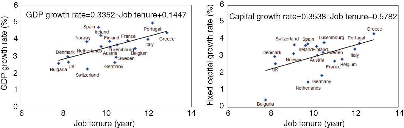
Economic growth, structural transformation and labor market institutions.
The country-specific average job tenure data, obtained from the OECD employment database, is estimated by the average length of time employees have been in their current main job for the period of 1970–1990. The GDP per capita growth rate (%) and fixed capital growth rate (%) are based on the average growth rate during 1970–1990 obtained from the World Bank database. Out of 34 observations from each OECD member country, the OECD database reports the average job tenure of 24 countries. We merge the dataset with economic growth measures in World Bank database, which reduces the sample observation to 18. The slope coefficient in each regression analysis is statistically significant at 99 percent level in the left panel and 95 percent level in the right panel. Detailed data descriptions and regression analysis are provided in the Appendix.
Motivated by the aforementioned empirical facts, we construct an endogenous growth model[1] of a small open economy having agricultural and non-agricultural sectors populated by a continuum of entrepreneurs and workers. Entrepreneurs employ capital and labor input to produce products in their respective sectors. Each sectoral labor market is subject to search and matching friction, as in Mortensen and Pissarides (1994). Employed workers provide labor and earn wages in the respective sectors, according to the Stole and Zwiebel (1996) bargaining rule, and accumulate human capital through learning-by-doing on the job. Unemployed workers collect unemployment benefits, search for jobs, and switch to the other sector when migration results in positive net gains. We assume the population and labor-augmenting technology (general human capital) of workers to grow at a constant rate. Analyzing the transition path from initial states to balanced growth paths under rational expectation enables us to investigate rich counterfactual scenarios. To solve for the entire transition path, we iterate the forward- and backward-shooting algorithms following Lipton et al. (1982) and Ishimaru, Oh, and Sim (2013).
We calibrate the model using the structural transformation episode of Japan. In addition to Japan, so called newly industrializing countries (NICs) of East Asia, such as Hong Kong, Singapore, South Korea, and Taiwan, have experienced rapid economic growth by transforming from agricultural to non-agricultural economies through specialization in heavy chemical industries. It is an interesting question why such rapid structural transformation to those heavy chemical industries took place in only those NICs and Japan. At least part of the answer likely lies in interaction between human capital accumulation and the “lifetime employment system” that resulted from the Confucian tradition which ethically discouraged job turnover by employees and dismissal by employers.[2] The interaction between human capital and lifetime employment system has little effect on the agricultural economy, which does not rely on significant (physical or human) capital accumulation. Rather it accelerates and intensifies specialization toward the non-agricultural sectors that require skilled workers and physical investment on complicated facilities, such as the electronics, automobiles, and heavy-chemical industries. In light of this, the main goal of our calibration is to quantify to what extent the lifetime employment system stimulates investment and enhances economic growth.
The counterfactual experiment finds that had the job durations of a typical worker been 1 year (roughly one tenth of the actual average job duration) for 1960–1990 in the Japanese labor market, the non-agricultural employment share in 1990 would have accounted for 81 percent of their actual values and the non-agricultural GDP per capita in 1990 for 71 percent of their actual values, respectively, suggesting sluggish structural transformation. Also, if the Japanese labor markets had transplanted from the flexible US labor market[3] the matching technology and high separation rate, non-agricultural GDP per capita would have been lower by 8 percent, whereas agricultural GDP per capita would have not been affected significantly. It suggests that at least during the period of structural transformation from agricultural to non-agricultural, the stable labor markets can perform better than flexible ones.
This paper adds to the extant literature on structural transformation several distinctive features. First, it introduces imperfect mobility of productive resources, that is, labor. Previous papers on structural transformation including Hansen and Prescott (2002), Ngai and Pissarides (2007), Duarte and Restuccia (2010), and Buera and Kaboski (2012) assume perfectly competitive labor markets absent any rigidity in factor mobility. Departing from the “immediate full employment assumption,” we borrow the concepts of both search friction from Mortensen and Pissarides (1994), Mortensen and Pissarides (1998) and an inter-sectoral labor barrier from Hayashi and Prescott (2008).[4] The current paper analyzes the dynamic path of non-stationary economic growth impeded by intra- and inter-sectoral labor rigidity. In our model, intra-sectoral rigidity (search friction) determines the direction of, and inter-sectoral rigidity (inter-sectoral barrier) determines the speed of, the non-stationary structural transformation.
Second, it incorporates both general and specific human capital. General human capital represents the accumulated knowledge or general equipment of the economy. Although not many workers in 1960 knew how to use automobiles, computers, or even telephones, most workers in developed countries now take advantage of cars, computers and cell-phones. These are captured by labor augmenting technology (general human capital) in our model. It works as a permanent TFP shock in other papers analyzing a balanced growth path with a permanent TFP shock. In addition to general human capital, workers individually acquire skills through learning-by-doing in many workplaces. The acquired skills through repetition of similar tasks may be specific to the occupation, job, or working environment. We capture it as job specific human capital of individual workers. Our numerical exercises quantify the effect of general human capital on the overall growth of the economy and that of specific human capital on the unbalanced growth of the sectors, structural transformation.
Third, rather than assuming an exogenously embedded TFP shock, the present paper demonstrates the endogenous structural transformation in the presence of labor market rigidity. Hayashi and Prescott (2008), and Uy, Yi, and Zhang (2013) analyze the structural transformation episode of Japan and South Korea.[5] In their models, however, the main driving force of structural transformation is the exogenously embedded sectoral TFP shock. In sharp contrast, this paper focuses on the dynamic path of the transitory equilibria which is endogenously determined by forward-looking decisions of contemporary economic agents having rational expectation. In the counterfactual experiments, we focus on to what extent the investment decisions by the forward-looking entrepreneurs encouraged by low labor cost has accelerated economic growth.
The remainder of the paper is organized as follows. We develop the model in Section 2 and, present numerical analysis using the Japanese episode in Section 3. Based on the calibration in Section 3, we conduct counterfactual experiments in Section 4, and conclude in Section 5.
2 The baseline model
2.1 Environment
Consider a small open economy populated by continuum of entrepreneurs and workers who consume both agricultural and non-agricultural products.[6] Entrepreneurs in both sectors, denoted by subscript i∈{a, m}, manage their own firms and take profit flow πt at every instant t∈[0, ∞). Workers are either employed or unemployed, the latter in both sectors receiving the same unemployment insurance, bt, at every instant, the employed workers in sector i earning wage wijt at time t, depending on skill j∈{h, l}. The labor market is assumed to be subject to search and matching friction following the Diamond-Mortensen-Pissarides model. Time is continuous and all economic agents discount the future at rate r.[7]
Workers At every instant, each individual worker having income flow w̅t chooses the consumption bundle (cat, cmt) to maximize
subject to the budget constraint pacat+pmcmt=w̅t, where pa and pm represent the world prices of agricultural and non-agricultural products, respectively.[8] It is assumed that workers are allowed neither to save nor to borrow.[9] Since we are looking at a small open economy, we assume that (pa, pm) are exogenously given and constant over time.[10] In particular, we take the non-agricultural products as numéraire and normalize pm to be unity. Note that the elasticity of substitution should be strictly positive, σ>0.[11] Solving the static utility maximization problem and plugging the individual demand for each product into the direct utility flow yields the indirect utility flow, as follows.
Denote by Lt the total population of workers at time t∈[0, ∞). At every instant, ρLt measure of workers retire and χLt measure of newly born workers enter the labor market as unemployed, which implies that the total population grows at rate χ–ρ(≥0) at every instant. Hence,
The sectoral ratio of newly-born workers is ex ante assumed to be the same as that of existing workers at every instant. But the new workers in one sector can immediately switch to the other sector at switching cost s~Logistic (0, εt/ω). For simplicity, the location parameter of the logistic distribution is normalized to be zero. The scale parameter of the logistic distribution is composed of parameter ω and the labor-augmenting technology εt (The role of the labor-augmenting technology will be explained later). Following Mcfadden (1974), Rust (1987), and Kennan and Walker (2011), we obtain the probability that the newly-born unemployed worker in sector i switches to sector –i as follows.
where Uit represents the lifetime value of the unemployed worker in sector i at time t.[12] Unemployed workers retire at rate ρ and receive job offers at rate f(θit).[13] If employed, the worker enjoys the lifetime value of Wilt. Unemployed workers in sector i also get revision shocks at rate ξ[14] and switch to the other sector if the net gains from doing so is positive. The Hamilton-Jacobi-Bellman (HJB hereafter) equation for the worker is given by
where
The detailed derivation of (6) is presented as well in Ishimaru, Oh, and Sim (2013). The left-hand side of (5) can be interpreted as the opportunity cost of holding the asset, unemployment at time t. The terms on the right-hand side represent the dividend flow from holding the asset Uit, the potential loss from retirement, the potential gains from job finding, the potential gains from inter-sectoral migration, and the gains from changes in valuation of the asset, respectively. To ensure the existence of the balanced growth path, we assume, following Mortensen and Pissarides (1998), that bt=bεt. An unskilled worker employed in sector i receives wage flow wilt per instant. The worker is separated from the job and becomes unemployed at rate δ and acquires skills at rate ζ. The HJB equations for the skilled and unskilled worker in sector i are, respectively,
The left-hand sides of (7) and (8) represent the opportunity cost of holding asset Wiht and Wilt, respectively. The right hand side in equation (7) consists of the dividend flow from the asset, the potential loss from retirement, the loss from job separation, and the gains from changes in valuation of the asset, respectively. The right hand side of (8) has one additional term, gains from skill acquisition. Note that employed workers are not allowed to search for another job, which reflects the scarcity of job-to-job transition in the Japanese labor market.[15] It is assumed that “skill” is job-specific so that skilled workers as well as unskilled workers lose their skill and get Uit when they are separated from their job.[16] Alternatively, one can think of a variant with “general skills,” which requires to extend the dimension of the model. The alternative may cause quantitative changes in our argument, but the qualitative implication of this paper will be maintained. Furthermore, in Japan, South Korea, and other East Asian countries having the Confucianism tradition, it is not common for an ordinary worker in one firm to switch to another rival firm and utilize the skills that she/he acquired in the former job. Once she/he is separated from a job, the worker is more likely to get the next job in a different occupation through long unemployment periods. Hence, this paper keeps the specific skills.
Entrepreneurs There are ni-measure of entrepreneurs in sector i∈{a, m}, who share the same preferences with workers. Entrepreneurs in each sector produce homogeneous products using identical production technology, given by
where
The total factor productivity component, ait, can be formed gradually through R&D investment and interaction with other productive resources (i.e. human capital). Throughout the paper we call it “technology.” That many R&D outcomes including new technologies and equipment can be utilized together with a certain level of skills accounts for gradual and persistent economic growth in a transitional economy. We posit
where λi is the efficiency parameter of technology investment, κi is the elasticity of technology investment, and ηa is the technology deterioration rate. Liht, Lilt, and Lit are the number of the skilled employed, unskilled employed, and all workers, respectively, in sector i at time t. Each entrepreneur in sector i makes R&D investment of zit at every t. The law of motion in (11) implies that that R&D investment becomes more efficient as the skilled population in sector i increases (human capital externality).[17] This, together with deterioration, embodies the gradual formation of the Ricardian comparative advantage and disadvantage. The capital stock, which can be immediately accumulated by purchasing from the international capital market, is depreciated at rate ηk.
where xit is the capital investment in sector i at time t. Regarding the labor input, it is assumed that
where (lilt, liht) represent the masses of unskilled and skilled workers, respectively, employed by the entrepreneur at time t. The coefficient αi reflects the fact that a skilled worker produces αi(≥1) times more than an unskilled worker. Again, “skill” is assumed to be job-specific. Let vit be the number of vacancies waiting for unemployed workers. The entrepreneur finds at rate q(θit) a worker who starts producing as an unskilled worker. Unskilled workers get learning shocks at rate ζ on the job and become skilled workers. All workers leave the entrepreneur due to separation shock at rate δ and retirement shock at rate ρ. The law of motion of the employed workers is described by
The profit flow of the entrepreneur in sector i at time t is given by
where (pk, pz) represent the cost of capital investment and R&D investment, respectively, and γεt represents the cost of creating a vacancy. Following Mortensen and Pissarides (1998), we assume the vacancy creation cost to grow together with εt, which is necessary to ensure the existence of the balanced growth path. The entrepreneur in sector i having (ε̅, a̅i, k̅i, l̅hi, l̅li) at time t chooses the schedule of (xiτ, viτ, ziτ) for each τ∈[t, ∞) to maximize
subject to (10), (11), (12), (14), (15) and the initial condition (εt, ait, kit, liht, lilt)=(ε̅, a̅i, k̅i, l̅hi, l̅li). Lemma 1 solves the optimal control problem by the entrepreneur.
Lemma 1:The entrepreneur in sector i∈{a, m} optimally chooses (xit, vit, zit) for each t∈[0, ∞) such that
In equations (18), (19), and (20), the left-hand side represents the marginal cost of investment, while the right-hand sides represent the marginal benefit. The proof of Lemma 1 is delayed in Appendix A.
Labor market The degree of the labor market tightness in sector i is defined as the ratio of the measure of total vacancy to that of job seekers in the sector. For each i∈{a, m},
Let m(vitni, uit) be the number of matches successfully formed at time t for each i∈{a, m}. Given constant returns to scale matching technology, we obtain
We denote by (Liht, Lilt, uit) the measure of skilled employees, unskilled employees, and unemployed workers, respectively, in sector i at time t. The total population, Lt, at time t is given by
The dynamic worker flows are summarized as follows.
where Lt is presented in (3). The last term of the right-hand side of (26) is derived by the following argument: At time t, there are χ(Laht+Lalt+uat) -measure of newly born workers in the agricultural sector and χ(Lmht+Lmlt+umt) -measure of newly born workers in the manufacturing sector; because they can immediately switch, the total measure of newly born workers in sector i after the immediate switching is given by χωitLt.
Wage bargaining In accordance with Stole and Zwiebel (1996),[18] successfully matched workers and entrepreneurs individually negotiate wages by splitting the marginal surplus.[19] This implies that for each j∈{h, l},
where ϕ is the worker’s bargaining power. In wage bargaining, the firm takes 1–ϕ portion of the joint (marginal) surplus and gives ϕ portion to the worker in the form of wage payment. Note that (27) is implicitly based on an equilibrium restriction such that in any equilibrium Wijt–Uit≥0 and
Lemma 2:The implied wage in sector i∈{a, m} is given by
where
Note that in both (29) and (30) the first terms are proportional to the marginal product of labor. The second terms reflect the labor market condition. For later use, we remark that
Equilibrium We finish this section by defining the equilibrium of our interest. The following definition summarizes the overall shape of our model.
Definition An equilibrium consists of bounded time series of choice rules {ωit, xit, vit, zit}i∈{a,m}, labor market tightness parameters {θit}i∈{a,m}, wages {wit}i={a,m}, value equations {Eit, Wiht, Wilt, Uit}i∈{a,m}, and laws of motions {εt, ait, kit, liht, lilt, Lt, Liht, Lilt, uit}i∈{a,m} at every t∈[0, ∞) such that:
unemployed workers as well as newly born workers optimally choose where they work when they are hit by an exogenous shock,
each entrepreneur in sector i optimally chooses {zit, xit, vit} at every t,
aggregate consistency requires that
the market tightness {θit}i∈{a, m} should be consistent with its definition,
wages {wit}i∈{a, m} should be consistent with the imposed bargaining rule,
Liht=niliht, Lilt=nililt, and Lt=∑i(Liht+Lilt+uit) for each i∈{a, m}.
the evolution of the entire system is recursively governed by the law of motions of (3), (5), (7), (8), (10), (11), (12), (14), (15), (17), (24), (25), and (26), given {Ei0, Wih0, Wil0, Ui0}i∈{a,m} and {ε0, ai0, ki0, lih0, lil0, L0, Lih0, Lil0, ui0}i∈{a, m}.
2.2 On the balanced growth path
In this subsection, we characterize the balanced growth paths by applying the previous definition with a small modification on the law of motions (v). Stationarity on the balanced growth path requires that
Let Lih, Lil and ui denote the proportion of skilled, unskilled and unemployed workers, respectively, in sector i to the total population. That is,
By the stationarity condition of the balanced growth path (31), these ratios are constant over time. The stationarity condition dictates that Δit/εt is constant over time on the balanced growth path. Also, from (15), (21), and (31), we get
on the balanced growth path. Since Lilt and uit grow together at the rate (χ–ρ), θit should be constant on the balanced growth path to make the last equality hold over time. We drop the time subscript t from the variables that are constant on the balanced growth path.
Using (31), we rewrite (5) as follows.
Combining (20) and (27) yields
Subtracting Uat from Umt, dividing by εt, and combining with (35) yields
These imply that (ωa, ωm) and (Umt–Uat)/εt are constant over time on the balanced growth path and uniquely determined by (θa, θm). From (25), (26), and (31), the triplet of (Lih, Lil, ui) is characterized as follows. Given (θa, θm), for each i∈{a, m},
Solving (37), (39) and (40), and multiplying by Lt results in Lemma 3.
Lemma 3:Given (θa, θm), on the balanced growth path,
Notice that
Lemma 4:Given (θa, θm) on the balanced growth path, the entrepreneur in each sector optimally chooses
where
In addition, these imply that
Plugging (42), (48), and (49) into (20) and reordering yields
for each i∈{a, m}. As mentioned before, (35) is based on the implicit restriction such that Wit–Uit>0 and
Proposition 1:There exists a balanced growth path if and only if the system of equations described in (50) has a solution of (θa, θm).
Given the complexity of the overall system, it is difficult to analytically determine under what parametric condition the balanced growth path exists and whether it is unique. Instead, we acknowledge that in our numerical experiment with reasonable parameter values, we obtain the same result regardless of the random starting points (we repeat the same experiment with more than 20 different random initial guesses).
2.3 On the postwar transition
Here, we characterize the transition path from a particular initial state to the balanced growth path, with the evolution of the economy governed by the system of differential equations. One advantage of our model is that the transition path is fully described by an autonomous control.
The lifetime value of unemployment evolves as follows. For each i∈{a, m},
Given (θat, θmt), equation (51) together with (6) determines (Uat, Umt, Δat, Δmt) at every t∈[0, ∞). Plugging (51) into (4) also yields (ωat, ωmt). Starting from (Lah0, Lal0, Lmh0, Lml0, ua0, um0), (Laht, Lalt, Lmht, Lmlt, uat, umt) evolve following (24)–(26) toward
Note that liht=Liht/ni, and lilt=Lilt/ni.
Lemma 5:Given (θat, θmt, Laht, Lalt, Lmht, Lmlt) at every t∈[0, ∞), we obtain
where
Lemma 5 summarizes the dynamic path followed by entrepreneurs. Given (θat, θmt) at every t∈[0, ∞), equations (24)–(26) jointly determine (Laht, Lalt, Lmht, Lmlt, uat, umt) and, together with Lemma 5, the unique path of the economy. Combining (20) and (27) yields
which restores (θat, θmt) at every t∈[0, ∞). Because (Wilt, Uit)→(Wil, Ui), we can get the convergence point (θa, θm). As in the previous subsection, (56) raises the equilibrium restriction that Wilt–Uit>0 for all i and t. Equations (24)–(26) and (51)–(56) provide the full description of the transition path of the model.
Again, the complexity of the system prevents us from providing an analytical proof on the existence and uniqueness of the solution. Instead, we acknowledge that we obtain the same result when we repeat the experiment with 20 different sets of “initial guesses.”
3 Numerical analysis
This section presents a quantitative assessment of the underlying link between labor market institutions and economic growth, with a focus on Japan. The Japanese episode is a comprehensive example of economic growth through structural transformation up to the starting point of “lost decades.” Lack of data for the 1950s and 1960s precludes analysis of the initial periods of structural transformation independently of the “postwar effect” of World War II (1939–1945) and the Korean War (1950–1953).
In Subsection 3.1, we calibrate the model by combining three Japanese data sources: the World Bank database; the Japanese national account; and the dataset employed by Hayashi and Prescott (2008). Lacking earlier data, we focus on the period beginning in 1960 and, to exclude the lost decades of Japan in the 1990s,[20] ending in 1990. Tables 1 and 2 summarize our choices of parameter values associated with Japan’s structural transformation.
Parameter values: exogenously assigned.
| Parameters | Description (source/target) |
|---|---|
| r=0.0095 | Discount rate (Esteban-Pretel and Sawada 2014) |
| pa/pm=1.2 | Price of agriculture good (Engel coefficient) |
| ρ=0.011 | Retirement rate (retirement age) |
| χ=0.014 | Birth rate (population growth rate) |
| δ=0.02 | Separation rate (Esteban-Pretel and Fujimoto 2012) |
| q(θ)=0.6θ−0.6 | Matching technology (Kano and Ohta 2002) |
| ϕ=0.6 | Bargaining parameter (Hosios 1990) |
| ψ=0.007 | Growth rate of the labor augmenting technology (average growth rate of OECD countries) |
| ηa=0.041 | Technology depreciation rate (Jorgenson 1996) |
| ηk=0.033 | Capital depreciation rate (Jorgenson 1996) |
| σ=3.8 | Elasticity of substitution (Ishimaru, Oh, and Sim 2013) |
Parameter values: endogenously targeted.
| Parameters | Description (source/target) | |
|---|---|---|
| ω=0.03 | Sensitivity of inter-sectoral migration | |
| ξ=0.007 | Arrival rate of revision shock | |
| αa=1.05 | Agr labor Productivity | |
| αm=1.5 | Non-Agr labor Productivity | |
| ζ=0.6 | Human capital accumulation | (The time series of sectoral GDP growth, sectoral labor share, sectoral capital share, sectoral wage growth, net EXP/GDP ratio, replacement ratio, and unemployment rate) |
| γ=0.12 | Cost of vacancy | |
| pk=0.3 | Capital cost | |
| pz=0.4 | Technology investment cost | |
| βka=0.193 | Agr capital share in production | |
| βkm=0.23 | Non-Agr capital share in production | |
| βla=0.58 | Agr labor share in production | |
| βlm=0.5 | Non-Agr labor share in production | |
| λa=0.3 | Efficiency of technology investment | |
| λm=0.5 | Efficiency of technology investment | |
| κa=0.1 | Elasticity of technology investment | |
| κm=0.4 | Elasticity of technology investment | |
| b=1.3 | Unemployment benefit |
3.1 Japanese structural transformation
Exogenously fed parameters We set r=0.0095 during the sample period to fix the annual interest rate at 3.8%, which is consistent with the estimate of the annual discount rate in Esteban-Pretel and Sawada (2014). But, the discount rate does not have a pronounced effect on the macro variables in our model. We normalize the price of non-agricultural products to be 1, and fix the relative price of agricultural products at 1.2, which is consistent with the average of the Engel coefficient from 1960 to 1990. The Engel coefficient, the ratio of food expenditures to total expenditures by households, is obtained by
Japan’s Engel coefficient was around 0.49 in 1960 and declined continuously to around 0.25 in 1990.[21] Because it assumes homothetic preferences, our model predicts a constant Engel coefficient, unless it additionally assumes the subsistence level, as in Matsuyama (1992). For the sake of simplicity, we alternatively take a simple average of the Engel coefficient during the target period.
The retirement rate is set to be 0.011, which results in roughly 90 percent of workers, who enter the labor market at age 25, retiring before age 70. The implied average “market duration,” the average elapsed time between labor market entry and exit, is thus less than than 25 years. Not being a life cycle model with aging, our model considers a worker who moves into the non-labor force to be a retiree and a worker who moves from the non-labor force into the labor force to be a newly born worker. Average market duration is thus much shorter than average lifespan. Japan’s population grew from 58.63 million in 1965 to 81.0 million in 1990.[22] The implied quarterly growth rate is ln(81.0/58.63)/100≈0.003, which determines the birth rate χ=ρ+0.003=0.014 during the sample period. The separation rate δ is set to 0.02 to obtain the average job duration of 12.5 years among non-retirees in the OECD data set. This choice is consistent with Esteban-Pretel and Fujimoto (2012). We posit
borrowing from Kano and Ohta (2002), who estimate the matching function of the Japanese labor market consistent with the plausible range of empirical elasticity of 0.5–0.7 proposed by Petrongolo and Pissarides (2001). We equalize the bargaining parameter to the elasticity of the matching technology by invoking Hosios’s condition, that is, ϕ=0.6. These choices on bargaining parameter and matching function parameters are consistent with Esteban-Pretel and Fujimoto (2012). The growth rate of labor augmenting technology ψ is set at 0.007. The latter choice, which implies a balanced growth path of 0.028 annually, is based on the average annual growth rate (a weighted average of country growth rates) of GDP in all OECD countries for the period 1980–1990.[23]
The capital depreciation rate ηk, calculated as the ratio of depreciation to real capital stock each year, results in ηk=0.033, following Jorgenson (1996).[24] Calculating the technology depreciation rate ηa based on the depreciation rate of service industry equipment results in ηa=0.041, again following Jorgenson (1996). Due to the lack of sectoral data, we employ the aggregate economy level of the depreciation rate. The elasticity of substitution σ is set to 3.8, following Bernard et al. (2003), Felbermayr, Prat, and Schmerer (2011), and Ishimaru, Oh, and Sim (2013). Values exogenously assigned are summarized in Table 1.
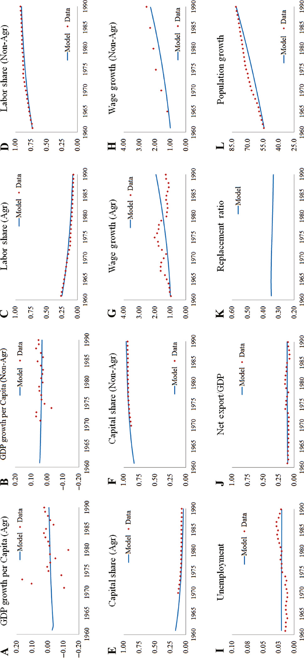
Calibrated parameters For the remaining parameters, we choose a vector that matches the aggregate of the time series data for sectoral GDP growth per capita, sectoral labor share, sectoral capital share, sectoral wage growth, the net EXP/GDP, replacement ratio and average unemployment rate.[25]
In Figure 2, the dots represent actual data values, the smooth lines the time series predicted by the model. Overall, Figure 2 suggests that our calibration strategy captures fairly well the trend in transition. Panels (A) and (B) present the time-series data and the model’s prediction of sectoral GDP growth per capita from 1970 to 1990 (lacking data for earlier periods). Panels (C) and (D) report sectoral labor shares, Panels (E) and (F) sectoral capital shares, from 1960 to 1990. Both labor and capital shares declined sharply in the agricultural, and rose rapidly in the non-agricultural, sector. In Panels (G)–(H), we exploit the evolution of sectoral wages from 1960 to 1990 to calibrate the labor productivity parameters (αa, αm, ζ). Based on historical wage data reported by Japan’s Ministry of Health, Labor and Welfare,[26] from 1960 to 1990 workers’ real wages grew by 29 and 152 percent in the agricultural and non-agricultural sectors, respectively. Panel (I) reports the unemployment rate in the actual data and the model. Without business cycle fluctuation, we set the target of the average unemployment rate at 2.0 percent. Panel (J) shows the Net Export/GDP ratio predicted by the model to be reconciled with the average Net Export/GDP ratio of 10.5 percent and its linear trend from 1960 to 1990. Panel (K) presents the population growth from the data and the model. Panel (l) reflects adjustment of the model’s parameters to keep unemployment benefits at around 40 percent of the average wage over time.[27] These choices are summarized in Table 2.
Calibration results (Japan).
4 Counterfactual experiments
Using the calibrated model, we conduct counterfactual experiments by substituting different arrival rates of separation shock and matching technologies. The baseline simulations, represented by the solid lines, are the results with the calibrated parameters. In the first counterfactual experiment, represented by the dotted lines (Counterfactual Experiment 1, or CE-1), setting the separation rate at 0.239 and retirement rate at 0.011 results in a 1-year job tenure.[28] The second experiment, represented by the dashed lines (Counterfactual Experiment 2, or CE-2), posits the counterfactual question: “If the Japanese labor market had transplanted from the flexible US labor market the efficient matching technology and high separation rate, what would have happened in 1990?”[29]
Figure 3 shows how varying job duration affects human capital accumulation and labor productivity, as calculated in each counterfactual experiment. Long job duration enables each entrepreneur to maintain high employment at a lower cost, and improves the average productivity of employed workers through learning-by-doing on the job. Panels (A)–(B) show the fraction of skilled workers to trend downward in the agricultural and upward in the non-agricultural sectors, and to be lower in counterfactual experiments involving a high separation rate. Panels (C)–(D) show the fraction of unskilled workers to exhibit moderate changes over time, Panels (E)–(F) labor productivity to be substantially higher in the baseline simulation.
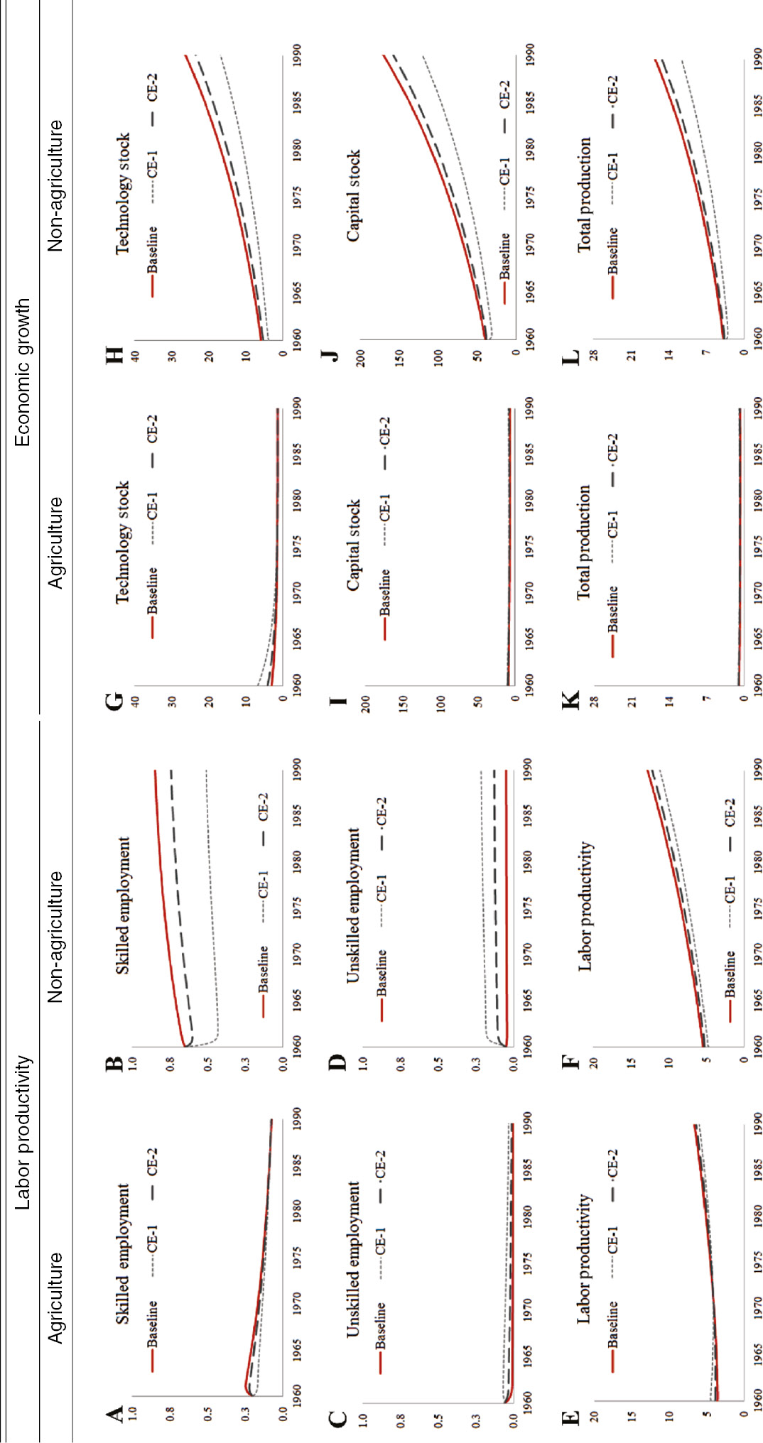
Counterfactual experiments: Japan (1960–1990).
Figure 3 also shows the transitional paths of technology stock, capital stock, and total production, as determined in each simulation. Panels (G)–(J) show agricultural investments in technology and capital to be slightly lower, and non-agricultural investments to be substantially lower, in the counterfactual experiments than in the baseline simulation. That technology and capital accumulation are more pronounced in the non-agricultural than in the agricultural sector is important. Taken together with the sectoral human capital accumulation patterns depicted in Figure 3 shows long job tenure and enhanced labor productivity to stimulate technology and capital investment more greatly in the non-agricultural sector. Consistent with these results, Panels (K)–(L) show aggregate production to be higher in the baseline simulation than in the counterfactual experiments. GDP growth in the non-agricultural sector, in which human capital accumulation significantly improves labor productivity and encourages investment, is especially accelerated by long job duration.
Table 3 summarizes the main results of our numerical experiments in terms of key ratios of counterfactual simulation results to baseline simulation results in 1990. Panel (A) presents the results from the first counterfactual experiment (CE-1), in which we set the separation rate at 0.239 and retirement rate at 0.011 to make job tenure 1 year. This result shows that if the job duration of Japanese workers had been 1 year, the non-agricultural employment share in 1990 would have accounted for about 80 percent, and non-agricultural GDP per capita in 1990 for about 70 percent, of their actual values. This suggests that long job duration is a crucial determinant of structural transformation that enables the economy to achieve rapid growth by driving resource reallocation from the agricultural to the non-agricultural sector.
Counterfactual experiments.
| Japan (1990) | |||
|---|---|---|---|
| Agriculture | Non-agriculture | Aggregate | |
| Panel A. Experiment with δ=0.239 to fix the job tenure at 1 year | |||
| GDP per capita | 1.29 | 0.71 | 0.74 |
| Technology stock | 1.02 | 0.64 | 0.66 |
| Capital stock | 1.29 | 0.71 | 0.73 |
| Employment | 1.43 | 0.81 | 0.86 |
| High type labor | 1.06 | 0.60 | 0.64 |
| Low type labor | 10.34 | 4.39 | 4.75 |
| Panel B. Experiment with δ=0.089 and q(θ)=1.35θ−0.72 | |||
| GDP per capita | 1.09 | 0.92 | 0.93 |
| Technology stock | 1.01 | 0.90 | 0.90 |
| Capital stock | 1.09 | 0.92 | 0.93 |
| Employment | 1.13 | 0.97 | 0.98 |
| High type labor | 1.02 | 0.88 | 0.89 |
| Low type labor | 3.84 | 2.61 | 2.69 |
| Panel C. Experiment with δ=0.089 | |||
| GDP per capita | 1.08 | 0.90 | 0.91 |
| Technology stock | 0.99 | 0.87 | 0.88 |
| Capital stock | 1.08 | 0.90 | 0.91 |
| Employment | 1.12 | 0.94 | 0.96 |
| High type labor | 1.01 | 0.85 | 0.86 |
| Low type labor | 3.80 | 2.54 | 2.62 |
Panel (B) depicts the second counterfactual simulation model (CE-2), which shows that, whereas agricultural GDP per capita would have not been affected, non-agricultural GDP per capita would have been lower by 8 percent. At the level of the aggregate economy, the difference between the baseline simulation and CE-2 implies that lower job duration would have reduced total GDP per capita by 7 percent. The counterfactual analysis of technology stock, capital stock, and human capital accumulation provides an explanation for the gap in GDP per capita across different labor market institutions. We show technology and capital stocks in the non-agricultural sector to be significantly lower in CE-2 than in the baseline simulations. In CE-2, the sectoral accumulations of technology and capital in the non-agricultural sector are 90–93 percent of the baseline simulation result in Japan, and skilled labor in the non-agricultural sector declines by 11 percent, whereas unskilled labor in both sectors increases significantly. This indicates that high separation rates drive lower human capital accumulation.
Panel (C) illustrates the effect of only making job duration shorter, as in the US labor markets, without transplanting the matching technology. These counterfactual simulation results show GDP per capita to be lower than in the baseline simulation or CE-2, which indicates that a high exogenous separation rate would have had a greater impact, some part of which, however, would have been absorbed by the efficient matching technology in CE-2. Although the loss by 9 percent in GDP per capita is smaller than the loss in the previous experiment, the loss is economically considerable as it amounts 3000 dollars in terms of GDP per capita and 346 billion dollars in total GDP (in terms of 2000 US dollar).
5 Conclusion
We incorporate labor market friction and learning-by-doing into a transitional two-sector growth framework to create a new endogenous growth model for exploring the underlying link between labor market institutions and economic growth. As workers stay in their jobs longer, they become more productive through learning-by-doing, which concomitantly lowers the labor cost to entrepreneurs. Enhanced labor productivity stimulates physical capital investment by forward-looking entrepreneurs. When the economy specializes in a sector where learning-by-doing does not improve labor productivity significantly, such as the agricultural sector, economic growth is more moderate. When the economy shifts towards the industrialized sector, on the other hand, in which the effect of learning-by-doing is significant, a stable labor market with a long job duration stimulates and accelerates economic growth by encouraging investment as well as improving labor productivity.
In the numerical analysis, we apply our model to the East Asian episode of structural transformation. Those countries’ lifetime employment systems, borne of the Confucian tradition that ethically discourages job turnover by employees and imposes on employers the duty of continuing employment, contributes to the formation of Ricardian comparative advantage in the non-agricultural industrialized sector. The counterfactual experiment finds that had the average job duration of Japanese workers been 1 year, the non-agricultural employment share would have accounted for about 80 percent, and non-agricultural GDP per capita for about 70 percent, of their actual values in 1990, which suggests sluggish structural transformation. Had the Japanese labor markets transplanted and maintained the efficient matching technology and high separation rate of the flexible US labor market, non-agricultural GDP per capita in 1990 would have declined by 8 percent, and aggregate GDP per capita by 7 percent, respectively. Lengthy job tenure was apparently one of the key ingredients in the structural transformation towards the non-agricultural sector.
Overall, this paper studies the underlying link between labor market institutions and the economic growth in transitional economies by highlighting matches between particular labor market institutions and sectoral characteristics. We hope that it delivers useful implications for many developing countries that are currently experiencing or expecting structural transformation towards the industrial sector. One may ask if our model can account for the recent growth slowdown or stagnation in NICs and Japan. This paper focuses on the structural transformation in the Japanese labor market from 1960 to 1990, with an emphasis on “capitalization effect.” In contrast, the emergence after the 1990s of the new (highly value-added) service sectors, such as information technology, computer software, health, and financial industries, may further emphasize “innate ability” rather than “acquired skill” and require “efficient reallocation” rather than “lifetime employment.” It may give us a hint on why the Japanese economy had achieved a considerable success in the manufacturing sectors (Sony, Toyota, Cannon, Panasonic, Sharp and so on), but underperformed in the software industries, information technology industries, financial industries and so on. Potential requirements for different processes of human capital accumulation and/or different types of human capital, being beyond the scope of this paper, are left to future research.
Acknowledgments
We thank Pengfei Wang (the editor), anonymous referees, Seung Mo Choi, Shin-ichi Fukuda, Junichi Fujimoto, Hidehiko Ichimura, Soohyun Oh, Dan Sasaki, Michio Suzuki and all seminar participants at various conferences and workshops including 2014 APEA conference in Bangkok, 2014 Annual Conference of the Canadian Economic Association, Sungkyunkwan University, and University of Tokyo. Seung-Gyu Sim appreciates the hospitality of E. Han Kim and the Ross School of Business, University of Michigan, a substantial part of this study having been completed during his stay in Ann Arbor. Seung-Gyu Sim is also grateful for the financial support by JSPS core-to-core Program (B. Asia-Africa science platforms). All errors are our own.
Appendix
A Regression analysis
In this section, we provide direct empirical evidence for the key mechanism of our model by examining the relations between labor market institutions and economic growth during structural transformation from OECD member sample countries for the period of 1970–1990. The numerical analysis for the Japanese episode in this paper focuses on the period beginning in 1960–1990 when Japan experienced a rapid economic growth through structural transformation. However, due to the data limitation, the cross-country empirical analysis employs the part of this period from 1970. Specifically, we assess the link between country-specific job tenure and 1) GDP growth rate and 2) capital investment during this period.
We first obtain cross-country job tenure data from OECD employment database (Dataset: LFS–Employment by Job Tenure). The job tenure is measured by the length of time employees have been in their current main job. The data is restricted to the period of 1992–2014 and has a gap to structural transformation period of each country. However, since country-specific time series job tenure data shows a persistent pattern over time,[30] we construct a time-invariant measure of job tenure for each sample country based on their average job tenure from 1992 to 2014. Then, we calculate the average growth rate of 1) GDP per capita and 2) fixed capital formation for the period of 1970–1990 from World Bank database[31] to capture the speed of aggregate economic growth and capital investment through structural transformation.
We estimate OLS regression relating the average growth rate of GDP per capita and capital investment with our country-specific average job tenure. Out of 34 observations from each OECD member country, the database on job tenure covers 24 countries. Then we merge with economic growth measures from World Bank database, which reduces the sample observation to 18. In Columns (1)–(2) of Table 4, the dependent variables are the average growth rate of annual GDP per capita and the average growth rate of gross fixed capital formation, respectively. All standard errors are robust to heteroskedasticity. Coefficients marked ***, ** and * are significant at the 1%, 5% and 10% level, respectively.
Regression analysis on economic growth and job tenure.
| (1) GDP growth | (2) Capital growth | |
|---|---|---|
| Job tenure | 0.335*** | 0.354** |
| (4.56) | (2.29) | |
| Constant | 0.145 | –0.578 |
| (0.18) | (–0.34) | |
| Observations | 18 | 18 |
| R2 | 0.372 | 0.267 |
t-statistics are reported in parenthesis. ** and ***represent statistical significance at the 5% and 1% level, respectively.
Columns (1) and (2) in Table 4 shows that longer job tenure increases the speed of economic growth during the period of structural transformation. The results indicate that a longer job tenure increases GDP growth and capital investment, and the effects are statistically significant in 1–5% significance level and economically large. One standard deviation increases in job tenure (1.4 year) is associated with 0.47% increase in annual GDP growth rate and 0.50% increase in annual fixed capital investment. These magnitudes are about 13% of average annual GDP growth and 16% of average capital investment, respectively.
B Mathematical appendix
Proof of Lemma 1: The entrepreneur chooses (xiτ, ziτ, viτ) at every τ∈[t, ∞) to maximize
subject to
First, we ignore the non-negative restriction in the domain and solve for the optimal control problem. Then, we check if the optimal decision is binding. The Hamiltonian for the above problem is
The maximum principle implies that
From (B10),
Since the shadow price μa cannot diverge as τ→∞, Ca=0. Thus, we get
Then, plugging (B14) into (B7) yields
Along the similar reasoning, by combining (B8) and (B11), we get
From (B12) and (B13), we get
Plugging (B18) into (B9) yields
Finally, since
connecting (B19) and (B20) results in
Proof of Lemma 2: Let
By equation (B21) and (B22), we get as follows.
Rewriting this yields
The solution of the above differential equation is given by
where
Proof of Lemma 3: Rewriting (39) and (40) in matrix notation yields
The matrix on the left-hand side is non-singular. Multiplying the inverse matrix of it on both side yields (Lah+Lal, Lmh+Lml, ua, um). Since (χ+δ)Lih=ζLil for each i∈{a, m} on steady states, we get (Lah, Lal, Lmh, Lml, ua, um).
Proof of Lemma 4: Since
we get
and
From (19),
Then, reordering and dividing by dt yields
Finally, sending dt→0 and reordering results in
Plugging (B30) and (B31) into the expression of
Since Lih=lihni, Lil=lilni, and q(θi)vi=(χ+δ+ζ), we get (46).
Proof of Proposition 1: First, suppose that there exists a balanced growth path. The stationarity conditions dictate that θat and θmt should be constant on the balanced growth path. Then, by construction, equation (50) should be satisfied on the balanced growth path. Second, suppose that the system of equations described in (50) has a solution of (θa, θm). Then, by invoking Lemma 1 through 4, we know that any pair of (θa, θm) can generate the solution of the model satisfying the equilibrium configuration (i) through (iv). Therefore, the solution of (50) solves for the balanced growth path.
Proof of Lemma 5: By the same reasoning as in the proof of Lemma 4, we get
Since
we get
It completes the proof.
C Numerical algorithm
C.1 On the balanced growth path
In this appendix, we describe the computational algorithm for solving the balanced growth path. To start, guess {θa, θb}.
Given (θa, θm), we obtain (Umt–Uat)/εt and (ωa, ωm) using (4) and (36).
Let
If ∑i(RHSi–LHSi)2 is less than the preassigned tolerance level, go to step (c). Otherwise, using the Nelder and Meade method, update (θa, θm) and go back to step (a).
Given (θa, θm), solve for variables {Li, ui, wi, ki, xi, ai, zi, vi, Yi}i∈{a,m}.
C.2 On the transition path
In this subsection, we present the solution algorithm for the transitional path to the new balanced growth path. First, we analyze the transition path from an initial point to the autarky balanced growth path. Assume that the economy converges to the new balanced growth path within T. We already know both endpoints.
Pick up a sufficiently large amount of time for T and construct the set of evenly spaced grid points {t0, t1, …, tn}⊂[0, T].
Guess the entire transition path of (Lat, Lmt, uat, umt, Wat, Wmt, Uat, Umt, pat, pmt).
Take all the other series as given and calculate the new series of
Take all the other series as given and iterate the new series of (Ŵat, Ŵmt, Ûat, Ûmt) by the backward shooting and weighted updating procedure as in step (c).
Take all the other series as given and iterate the prices
Iterate step (c), (d), and (e), until all the series converge to the below of a certain tolerance level. If the differentials between the initial value and the updated values are small enough, move onto step (g).
Prolong the time interval into
References
Acemoglu, D., and W. B. Hawkins. 2014. “Search with Multi-worker Firms.” Theoretical Economics 9 (3): 583–628.10.3982/TE1061Search in Google Scholar
Aghion, P., and P. Howitt. 1994. “Growth and Unemployment.” Review of Economic Studies 61 (3): 477–494.10.2307/2297900Search in Google Scholar
Arrow, K. J., H. B. Chenery, B. S. Minhas, and R. M. Solow. 1961. “Capital-Labor Substitution and Economic Efficiency.” The Review of Economics and Statistics 43 (3): 225–250.10.2307/1927286Search in Google Scholar
Bernard, A. B., J. Eaton, J. B. Jensen, and S. Kortum. 2003. “Plants and Productivity in International Trade.” American Economic Review 93 (4): 1268–1290.10.3386/w7688Search in Google Scholar
Buera, F. J., and J. P. Kaboski. 2012. “Scale and the Origins of Structural Change.” Journal of Economic Theory 147 (2): 684–712.10.1016/j.jet.2010.11.007Search in Google Scholar
Chen, B.-L., H.-J. Chen, and P. Wang. 2011. “Labor-Market Frictions, Human Capital Accumulation, and Long-Run Growth: Positive Analysis and Policy Evaluation.” International Economic Review 52 (1): 131–160.10.1111/j.1468-2354.2010.00622.xSearch in Google Scholar
Choi, S. M. 2011. “How Large are Learning Externalities?.” International Economic Review 52 (4): 1077–1103.10.1111/j.1468-2354.2011.00660.xSearch in Google Scholar
Duarte, M., and D. Restuccia. 2010. “The Role of the Structural Transformation in Aggregate Productivity.” The Quarterly Journal of Economics 125 (1): 129–173.10.1162/qjec.2010.125.1.129Search in Google Scholar
Esteban-Pretel, J., and J. Fujimoto. 2012. “Life-Cycle Search, Match Quality and Japan’s Labor Market.” Journal of the Japanese and International Economies 26 (3): 326–350.10.1016/j.jjie.2012.06.003Search in Google Scholar
Esteban-Pretel, J., and Y. Sawada. 2014. “On the Role of Policy Interventions in Structural Change and Economic Development: The Case of Postwar Japan.” Journal of Economic Dynamics and Control40: 67–83.10.1016/j.jedc.2013.12.009Search in Google Scholar
Felbermayr, G., J. Prat, and H.-J. Schmerer. 2011. “Globalization and Labor Market Outcomes: Wage Bargaining, Search Frictions, and Firm Heterogeneity.” Journal of Economic Theory 146 (1): 39–73.10.1016/j.jet.2010.07.004Search in Google Scholar
Hansen, G. D., and E. C. Prescott. 2002. “Malthus to Solow.” American Economic Review 92 (4): 1205–1217.10.3386/w6858Search in Google Scholar
Hayashi, F., and E. C. Prescott. 2008. “The Depressing Effect of Agricultural Institutions on the Prewar Japanese Economy.” Journal of Political Economy 116 (4): 573–632.10.3386/w12081Search in Google Scholar
Helpman, E., and O. Itskhoki. 2010. “Labour Market Rigidities, Trade and Unemployment.” Review of Economic Studies 77 (3): 1100–1137.10.1111/j.1467-937X.2010.00600.xSearch in Google Scholar
Helpman, E., O. Itskhoki, and S. Redding. 2010. “Inequality and Unemployment in a Global Economy.” Econometrica 78 (4): 1239–1283.10.3386/w14478Search in Google Scholar
Hosios, A. J. 1990. “On the Efficiency of Matching and Related Models of Search and Unemployment.” Review of Economic Studies 57 (2): 279–98.10.2307/2297382Search in Google Scholar
Ishimaru, S., S. Oh, and S.-G. Sim. 2013. “Unemployment and Inequality after Trade Liberalization.” Discussion papers.Search in Google Scholar
Jorgenson, D. 1996. “Empirical Studies of Depreciation.” Economic Inquiry 34: 24–42.10.7551/mitpress/2577.003.0005Search in Google Scholar
Kano, S., and M. Ohta. 2002. “An Empirical Matching Function with Regime Switching: The Japanese Case.” Discussion paper, Institute of Policy and Planning Sciences, No. 967.Search in Google Scholar
Kennan, J., and J. R. Walker. 2011. “The Effect of Expected Income on Individual Migration Decisions.” Econometrica 79 (1): 211–251.10.3386/w9585Search in Google Scholar
Lipton, D., J. Poterba, J. Sachs, and L. Summers. 1982. “Multiple Shooting in Rational Expectations Models.” Econometrica 50 (5): 1329–1333.10.3386/t0003Search in Google Scholar
Lucas, R. J. 1988. “On the Mechanics of Economic Development.” Journal of Monetary Economics 22 (1): 3–42.10.1016/0304-3932(88)90168-7Search in Google Scholar
Matsuyama, K. 1992. “Agricultural Productivity, Comparative Advantage, and Economic Growth.” Journal of Economic Theory 58 (2): 317–334.10.3386/w3606Search in Google Scholar
Mcfadden, D. 1974. “Conditional Logit Analysis of Qualitative Choice Behavior.” In Frontiers in Econometrics, edited by P. Zarembka, 105–142. New York: Academic Press.Search in Google Scholar
Miyamoto, H., and Y. Takahashi. 2011. “Productivity Growth, on-the-Job Search, and Unemployment.” Journal of Monetary Economics 58 (6–8): 666–680.10.1016/j.jmoneco.2011.11.007Search in Google Scholar
Mortensen, D. T., and C. A. Pissarides. 1994. “Job Creation and Job Destruction in the Theory of Unemployment.” Review of Economic Studies 61 (3): 397–415.10.2307/2297896Search in Google Scholar
Mortensen, D. T., and C. A. Pissarides. 1998. “Technological Progress, Job Creation and Job Destruction.” Review of Economic Dynamics 1 (4): 733–753.10.1006/redy.1998.0030Search in Google Scholar
Ngai, L. R., and C. A. Pissarides. 2007. “Structural Change in a Multisector Model of Growth.” American Economic Review 97 (1): 429–443.10.1257/aer.97.1.429Search in Google Scholar
Petrongolo, B., and C. A. Pissarides. 2001. “Looking into the Black Box: A Survey of the Matching Function.” Journal of Economic Literature 39 (2): 390–431.10.1257/jel.39.2.390Search in Google Scholar
Pissarides, C. A., and G. Vallanti. 2007. “The Impact Of TFP Growth On Steady-State Unemployment.” International Economic Review 48 (2): 607–640.10.1111/j.1468-2354.2007.00439.xSearch in Google Scholar
Romer, P. M. 1986. “Increasing Returns and Long-Run Growth.” Journal of Political Economy 94 (5): 1002–37.10.1086/261420Search in Google Scholar
Romer, P. M. 1987. “Growth Based on Increasing Returns Due to Specialization.” American Economic Review 77 (2): 56–62.Search in Google Scholar
Rust, J. 1987. “Optimal Replacement of GMC Bus Engines: An Empirical Model of Harold Zurcher.” Econometrica 55 (5): 999–1033.10.2307/1911259Search in Google Scholar
Shimer, R. 2005. “The Cyclical Behavior of Equilibrium Unemployment and Vacancies.” American Economic Review 95 (1): 25–49.10.1257/0002828053828572Search in Google Scholar
Stole, L. A., and J. Zwiebel. 1996. “Intra-Firm Bargaining under Non-binding Contracts.” Review of Economic Studies 63 (3): 375–410.10.2307/2297888Search in Google Scholar
Uy, T., K.-M. Yi, and J. Zhang. 2013. “Structural Change in an Open Economy.” Journal of Monetary Economics 60 (6): 667–682.10.1016/j.jmoneco.2013.06.002Search in Google Scholar
©2017 Walter de Gruyter GmbH, Berlin/Boston
Articles in the same Issue
- Frontmatter
- Advances
- Global value chains and the exchange rate elasticity of exports
- Home hours in the United States and Europe
- Persistent vs. Permanent Income Shocks in the Buffer-Stock Model
- Contributions
- Business cycle synchronization across U.S. states
- Qualitative and quantitative central bank communication and inflation expectations
- Economic growth and labor market friction: a quantitative study on Japanese structural transformation
- The Feldstein-Horioka hypothesis revisited
- Human-capital spillover, population and R&D-based growth
- Inflation and the steeplechase between economic activity variables: evidence for G7 countries