When Experience Pays Off: Professional Development, Work Scheduling, and Performance
-
Guan-Yuan Wang


Abstract
Organizations routinely face scheduling decisions that affect worker performance, with rest and preparation being particularly crucial for high-intensity, performance-critical contexts. Yet little is known about how professional experience affects workers’ ability to adapt to variations in these preparation windows. We examine whether scheduling sensitivity varies with career experience, using variation in NBA game start times during the 2023–24 season to identify preparation constraints. Using fixed-effects models, we find that experienced players demonstrate superior performance when preparation windows are compressed, while younger players benefit more from extended preparation time. This suggests that accumulated professional experience enables better adaptation strategies through learning-by-doing. These findings highlight important considerations for competitive balance in sports leagues and suggest organizations may benefit from experience-differentiated scheduling policies that leverage experienced employees’ adaptation capabilities while providing structured preparation windows for newer workers.
1 Introduction
The relationship between sleep patterns and athletic performance has garnered significant attention in sports science research, with evidence demonstrating that strategic napping and optimal timing enhance physical and cognitive performance (Cook and Charest 2023; Haskell et al. 2025). Studies show that pre-competition naps improve reaction time, alertness, and overall athletic output among elite athletes (Teece et al. 2023a, 2023b; Boukhris et al. 2024; Waterhouse et al. 2007), with documented improvements in power and reductions in fatigue following strategic daytime sleep periods (Teece et al. 2023a, 2023b). NBA players consistently emphasize the critical role of pre-game naps, describing them as non-negotiable and typically napping for 2–3 h before games (NBA on ESPN 2023).
These findings align with broader workplace productivity research, where the same cognitive and physiological mechanisms underlying strategic rest benefit performance in high-intensity occupations (Li et al. 2021; Iridiastadi 2021; Onninen et al. 2020). Yet workplace research also reveals that scheduling patterns critically affect these rest benefits. Unstable schedules reduce productivity (Kamalahmadi et al. 2021; Kesavan et al. 2022) and increase distress (Schneider and Harknett 2019), while consistent schedules improve performance (Lu et al. 2022). When scheduling flexibility is available, it can enhance well-being and productivity (Angelici and Profeta 2024; Arntz et al. 2022; Mas and Pallais 2017), leading workers to seek schedule control in alternative arrangements (Chen et al. 2019; Bergman et al. 2023; De Menezes and Kelliher 2017).
Turning to basketball-specific research, studies examining game timing, often confounded with travel effects, show mixed findings regarding performance impacts. Nutting and Price (2017) found no significant relationship between time zones and team performance from 2002 to 2013. However, Hasbany et al. (2023) found that eastward travel increases team scoring via improved shooting performance, while Glinski and Chandy (2022) found that jet lag negatively affected free throw shooting only for westward travel, and Özdalyan et al. (2024) reported that westward travel increases performance while eastward travel decreases it. These studies focus primarily on team-level outcomes or specific skills, potentially masking important heterogeneity at the individual player level. Our study bridges workplace productivity and basketball-specific findings by examining how individual player performance varies with game timing across different career stages.
Our study bridges workplace productivity and basketball-specific findings by distinguishing between two types of scheduling challenges that affect player performance differently. Professional basketball players face scheduling constraints that arise from both travel logistics and game timing decisions. Travel-related factors, such as timezone crossing, impose physiological disruptions that teams attempt to mitigate by arriving the night before games to allow for rest and recovery (Bulls.com 2025). This travel planning acknowledges that physiological constraints from jet lag are a fundamental and often unavoidable biological burden.
In contrast, game start times represent a strategic dimension of scheduling where adaptation opportunities exist. Players describe structured preparation routines built meticulously around game timing, including optional morning shootarounds for shot preparation, post-lunch rest periods, and crucial pre-game naps timed to evening tipoffs (NBA on ESPN 2023; Bulls.com 2025). The goal, as one player noted, is to be prepared when game time comes by focusing on fundamentals and physical readiness (Bulls.com 2025). When games are scheduled for afternoon rather than the typical evening hours, these carefully developed routines must be compressed or strategically adjusted. This distinction between physiological disruptions from travel and strategic timing adaptation for game preparation provides a natural setting to examine how professional experience shapes an athlete’s ability to optimize performance across varying scheduling constraints.
To examine this individual-level variation, NBA scheduling provides a natural experiment for examining predetermined timing effects on performance. Most games are scheduled for evening hours, allowing players to develop consistent routines with strategic afternoon napping. When games are scheduled earlier, these routines must be adjusted. This preparation is explicitly viewed as critical for development: a player emphasizes the importance of utilizing optional pre-game work, stating, “The best way to be prepared is to put your work in before the game so you’re prepared when game time comes…especially as a young player” (Bulls.com 2025). This highlights the necessity for younger athletes to maximize the available time for practice, film, and physical readiness. Using comprehensive 2023–24 NBA season data, we investigate how game start times affect player performance across career stages. We classify players aged 28 and above as experienced, aligning with official NBA demographics showing average ages of 26–28 years (NBA 2024). We validate this threshold through robustness tests across ages 26–30.
We find that timing importance varies significantly by career stage. Younger players benefit from evening games providing extended preparation windows, consistent with pre-competition napping research. However, players aged 28 and above perform better in afternoon games, suggesting experience enables efficient adaptation when preparation windows are compressed. This interaction is robust across performance metrics, sample definitions, and age thresholds. Heterogeneity analysis reveals effects are strongest in contexts where adaptation skills matter most: away games, starting players, winning games, and among guards with the highest movement demands.
Our results contribute to the literature on strategic rest and workplace adaptation (Alfes et al. 2022; Ranasinghe et al. 2025) by providing field evidence for how career progression shapes timing flexibility and performance optimization strategies. From a sports economics perspective, these findings raise considerations for competitive balance, as teams with different age compositions may have systematic advantages depending on game scheduling (Wang et al. 2018; Karg et al. 2021; Schreyer et al. 2016; Schreyer and Ansari 2022). From a managerial perspective, our findings suggest human resource policies should consider experience-differentiated scheduling approaches, providing structure for newer employees while leveraging experienced workers’ adaptability across varied conditions (Hunter and Wu 2016; Baucells and Zhao 2019; Jeunet and Salassa 2024).
The paper proceeds as follows. Section 2 describes our data. Section 3 presents our empirical specification. Section 4 reports the main results. Section 5 concludes. Appendix A presents descriptive statistics of our sample data. Appendix B presents robustness checks, examining alternative performance metrics, sample definitions, and age thresholds. Appendix C presents heterogeneity analysis across player characteristics and game contexts.
2 Data and Sample
Our analysis uses comprehensive player performance and game scheduling data from the official data source, NBA API.[1] The dataset comprises player-level demographic information (age,[2] position, and team) and game-level performance data including detailed box score statistics. From these statistics, we construct our primary outcome measures: Efficiency (EFF) and Game Score (GmSc). EFF captures overall performance by summing positive actions (points, rebounds, assists, steals, blocks) and subtracting negative ones (missed shots, turnovers, fouls). GmSc, developed by basketball statistician John Hollinger, uses a similar approach but weights individual statistics differently. Both metrics are designed to measure player’s overall performance in a single game. Detailed formulas are provided in Kubatko et al. (2007) and Hollinger (2003).
Game start times serve as our primary explanatory variable, ranging from 12:00 PM to 9:00 PM local time. To address potential confounding from travel-related fatigue, we construct a timezone change variable measuring the difference between the game location and the team’s home city timezone, following suggestions from Nutting (2010) and Nutting and Price (2017). This variable typically ranges from −3 to +3 h for continental US travel, with negative values indicating westward travel (adaptation to later local times) and positive values indicating eastward travel (adaptation to earlier local times). The extreme values of 6 h reflect one of the NBA global games in international venues such as Paris.
Our sample includes all player-game observations from the 2023–24 NBA regular season (1,230 unique games across 30 teams), restricting to players appearing in at least 25 games with positive playing time. This ensures adequate exposure to timing variation while focusing on regular contributors, yielding 24,460 player-game observations. Table 3 in Appendix A presents descriptive statistics and correlations for key variables.
Figure 1 shows the distributions of key variables in our sample. Panel (a) displays the age distribution of players. Panel (b) shows that most games start between 6 and 8 PM local time, though some afternoon games begin as early as noon. Panel (c) presents the distribution of timezone changes, which cluster around zero, indicating that most games are played in or near the team’s home timezone.[3] Following Nutting and Price (2017), we examine the seasonal distribution of game start times. Figure 2 shows that day games (starting before 6 PM) are less common at the beginning of the season (October, 4.1 %) and more common at the end (April, 18.2 %). This seasonal variation motivates our inclusion of month fixed effects in the empirical analysis to control for time-varying factors that may correlate with both game start times and player performance.

Distribution of key variables. Panel (a) displays the age distribution of players. Panel (b) shows the distribution of game start times. Panel (c) presents the distribution of timezone changes.

Percentage of day games by month during the 2023–24 NBA season.
3 Empirical Specification
We employ a fixed effects regression framework to estimate how game start times affect player performance across age groups. Our identification strategy leverages variation in NBA game start times, which are predetermined by league scheduling based on broadcasting agreements, arena availability, and market considerations, and are not chosen in response to individual team characteristics such as player age composition. This ensures that our timing variation is plausibly exogenous to player-level performance factors. We explicitly control for time zone change effects to address travel-related fatigue. Our central hypothesis posits that younger players benefit from the extended preparation windows that evening games provide, while experienced players perform relatively better in earlier games through efficient adaptation strategies developed via learning-by-doing.
We classify players aged 28 and above as experienced, aligning with the average NBA player age and official league demographics (NBA 2024).[4] Our empirical analysis proceeds in three stages, progressively incorporating interaction terms to identify heterogeneous timing effects across career stages. First, we estimate the baseline relationship between game start times and performance, interacted with player experience:
where Performance ijt represents the performance measure for player i on team j at time t. Our primary outcome is Efficiency (EFF), supplemented by Game Score (GmSc) for robustness validation. Game_Start_Time jt is the numerical representation of game start time, allowing us to capture the continuous relationship between timing and performance. Timezone_Change jt controls for the timezone difference between the game location and the team’s home city, addressing potential confounding from travel-related fatigue that may otherwise bias our estimates of pure timing effects.
The vector X it includes game-level controls: Home_Game jt accounts for home field advantage; Pace jt captures game tempo and style; and Wins jt controls for team performance that might affect individual statistics. All specifications include player fixed effects (δ i ) and month fixed effects (θ t ), with standard errors clustered at both the player and team levels to account for potential correlation in performance within players across games and within teams across different games. Month fixed effects are particularly important because day games vary systematically across the season, as discussed in Figure 2. As a robustness check, we also estimate specifications with team fixed effects (results presented in Appendix B.1).
Second, we examine how timezone changes differentially affect performance across age groups:
This specification isolates the differential adaptation capacity to travel-related disruptions, with β 3 identifying whether experienced players mitigate jet lag effects more effectively than their younger counterparts.
Third, our full specification simultaneously estimates both interaction effects:
This comprehensive model allows us to jointly assess whether experience-based adaptation manifests differently across the two dimensions of scheduling constraints: strategic timing adjustments versus physiological travel disruptions.
4 Results
Before presenting our econometric analysis, we provide model-free evidence on the relationship between game timing and player performance across age groups. Figures 3 and 4 display the unconditional relationships between our key variables and performance outcomes, offering a visualization of the patterns that motivate our subsequent regression analysis.

Player efficiency by game start time and age group.

Player efficiency by timezone change and age group.
Figure 3 shows mean player efficiency ratings against game start times, separately for players below and above age 28. The data reveal a clear divergent pattern between younger and more experienced players. For younger players (Age < 28, shown in black), performance exhibits a gradual upward trend across the range of game start times, suggesting that later games may be beneficial for less experienced players. In contrast, older players (Age ≥ 28, shown in gray) demonstrate a clear decline in efficiency as game start times move later in the day. This divergent pattern provides strong preliminary evidence for age-differentiated responses to game scheduling that form the foundation of our empirical investigation.
Figure 4 examines the relationship between timezone change and performance across the same age groups.[5] The results reveal patterns similar to those observed for game start times: younger players show relatively stable performance across different timezone changes, while older players demonstrate better performance with eastward travel (positive timezone changes) and declining performance with westward travel. These patterns suggest that both game start times and timezone changes may interact with player experience in affecting performance. While both variables show similar age-related patterns, we focus our main analysis on game start times because they represent a direct management decision variable, whereas timezone changes primarily reflect travel logistics. Nevertheless, we control for timezone effects throughout our analysis and examine both variables in parallel in our empirical specifications.
Table 1 reports the player fixed-effects estimates examining how game start time affects player performance (Efficiency, EFF), and how this relationship varies by career experience. Figure 5 visualizes the key coefficients from Column (1) (without controls) and Column (4) (with controls), illustrating the direct effect of game start time and its interaction with the age ≥ 28 indicator.
Effect of game start time on player performance (EFF) by age.
| (1) | (2) | (3) | (4) | (5) | (6) | |
|---|---|---|---|---|---|---|
| EFF | EFF | EFF | EFF | EFF | EFF | |
| Game start time | 0.081 | 0.036 | 0.081 | 0.090c | 0.042 | 0.090c |
| (0.049) | (0.034) | (0.049) | (0.042) | (0.028) | (0.042) | |
| Game start time × age ≥ 28 | −0.111c | −0.110c | −0.120c | −0.120c | ||
| (0.064) | (0.064) | (0.066) | (0.066) | |||
| Timezone change | 0.094 | 0.103 | 0.102 | 0.023 | 0.031 | 0.030 |
| (0.062) | (0.075) | (0.075) | (0.054) | (0.068) | (0.068) | |
| Timezone change × age ≥ 28 | −0.024 | −0.021 | −0.022 | −0.018 | ||
| (0.115) | (0.114) | (0.115) | (0.114) | |||
| Home game | 0.230b | 0.231b | 0.230b | |||
| (0.088) | (0.088) | (0.087) | ||||
| Pace | 0.085a | 0.085a | 0.085a | |||
| (0.011) | (0.011) | (0.011) | ||||
| Win | 2.133a | 2.132a | 2.133a | |||
| (0.109) | (0.110) | (0.109) | ||||
| Observations | 24,460 | 24,460 | 24,460 | 24,460 | 24,460 | 24,460 |
| Controls | ✓ | ✓ | ✓ | |||
| Player FE | ✓ | ✓ | ✓ | ✓ | ✓ | ✓ |
| Month FE | ✓ | ✓ | ✓ | ✓ | ✓ | ✓ |
-
Standard errors clustered at the player and team level are reported in parentheses. Controls include home game indicator, pace, and win indicator. Pace measures the number of possessions per 48 min. Results remain consistent when using total possessions as an alternative control variable. a p < 0.01, b p < 0.05, c p < 0.1.
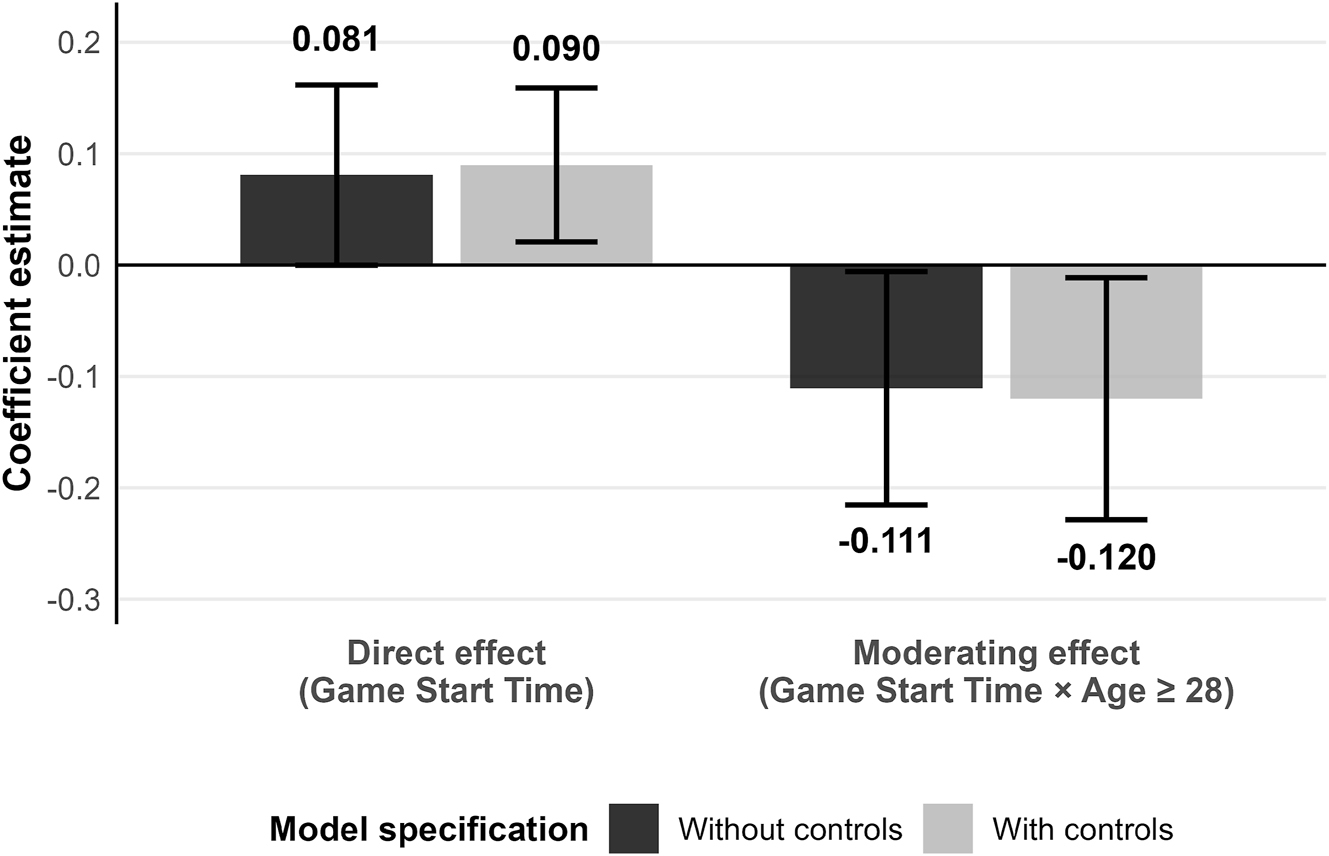
Effect of game start time on player performance: direct effects and moderating effects by age.
The results show a clear and consistent pattern. Later game start times are associated with higher performance for younger players, while the interaction term is negative, indicating that experienced players perform relatively better in earlier games. Specifically, in the baseline specification without controls, the effect of game start time is positive but statistically insignificant (0.081, p > 0.10), while the interaction term is negative and marginally significant (−0.111, p < 0.10). When game-level controls are added, the coefficient on game start time increases slightly to 0.090 (p < 0.10), and the interaction term remains negative and marginally significant (−0.120, p < 0.10). The stability of both sign and magnitude across specifications suggests that the moderating role of experience is robust and not driven by omitted factors.
Importantly, these effects are robust to the inclusion of game-level controls such as home advantage, pace, and team win outcome, which all show expected signs and significance. The inclusion of controls strengthens rather than weakens the main coefficients, suggesting that the results are not driven by confounding factors.
Timezone change and its interaction with age are small and statistically insignificant in all player fixed-effects specifications, providing no evidence that travel-related physiological disruptions affect players differently by age. Because these coefficients are not significant and not central to our theoretical argument, we focus on the timing-related effects visualized in Figure 5.
The control variables behave as expected: home games are associated with higher efficiency
Overall, the results support the interpretation that accumulated professional experience enables players to adapt efficiently when pre-game preparation windows are shortened. Younger players benefit from later start times that allow extended preparation, whereas experienced players achieve comparable or superior performance when games are scheduled earlier, consistent with learning-by-doing and refined schedule-management strategies.
To verify that our results are not driven by the choice of performance metric, Table 2 replicates our main analysis using Game Score (GmSc) as the dependent variable. The results exhibit consistent patterns across both performance measures, though with somewhat weaker statistical significance. The coefficient on game start time is 0.062 (p < 0.10), while the interaction term is −0.088, which is statistically insignificant (p > 0.10) in the player fixed effects specification. However, the direction and magnitude of effects remain consistent with our main findings using Efficiency as the outcome variable. Additionally, the findings remain robust when using team fixed effects specifications, which offer complementary identification by exploiting variation at the team level. As reported in Appendix B.1, the team fixed effects estimates yield similar yet stronger statistical patterns, with the game start time coefficient increasing to 0.136 (p < 0.01) and the interaction term remaining negative and highly significant (−0.246, p < 0.01).
Effect of game start time on player performance (GmSc) by age.
| (1) | (2) | (3) | (4) | (5) | (6) | |
|---|---|---|---|---|---|---|
| GmSc | GmSc | GmSc | GmSc | GmSc | GmSc | |
| Game start time | 0.056 | 0.023 | 0.056 | 0.062c | 0.027 | 0.062c |
| (0.037) | (0.026) | (0.037) | (0.032) | (0.022) | (0.032) | |
| Game start time × age ≥ 28 | −0.081 | −0.081 | −0.088 | −0.088 | ||
| (0.054) | (0.055) | (0.057) | (0.057) | |||
| Timezone change | 0.059 | 0.062 | 0.061 | 0.006 | 0.010 | 0.009 |
| (0.050) | (0.058) | (0.058) | (0.045) | (0.053) | (0.054) | |
| Timezone change × age ≥ 28 | −0.010 | −0.007 | −0.009 | −0.006 | ||
| (0.085) | (0.085) | (0.086) | (0.085) | |||
| Home game | 0.170b | 0.170b | 0.170b | |||
| (0.069) | (0.069) | (0.069) | ||||
| Pace | 0.056a | 0.056a | 0.056a | |||
| (0.008) | (0.008) | (0.008) | ||||
| Win | 1.601a | 1.600a | 1.601a | |||
| (0.086) | (0.087) | (0.086) | ||||
| Observations | 24,460 | 24,460 | 24,460 | 24,460 | 24,460 | 24,460 |
| Controls | ✓ | ✓ | ✓ | |||
| Player FE | ✓ | ✓ | ✓ | ✓ | ✓ | ✓ |
| Month FE | ✓ | ✓ | ✓ | ✓ | ✓ | ✓ |
-
Standard errors clustered at the player and team level are reported in parentheses. Controls include home game indicator, pace, and win indicator. Pace measures the number of possessions per 48 min. Results remain consistent when using total possessions as an alternative control variable. a p < 0.01, b p < 0.05, c p < 0.1.
Our main findings demonstrate robustness across multiple specifications and sample definitions. As detailed in Appendix B, results remain consistent when using team fixed effects (Appendix B.1 Team Fixed Effects Specification), alternative sample periods excluding October and April (Appendix B.2 Alternative Sample Period), more restrictive player selection criteria requiring at least 42 games, which represents approximately half of the 82-game regular season (Appendix B.3 Alternative Sample Selection), and different age thresholds ranging from 26 to 30 years (Appendix B.4 Alternative Age Thresholds).
Heterogeneity analysis (Appendix C) reveals that experience-based timing effects are strongest in contexts where adaptation skills matter most: away games where players face unfamiliar environments (Appendix C.1 Home versus Away Games), starting players with greater performance responsibilities (Appendix C.2 Starters versus Bench Players), and guards with the highest cognitive and physical demands (Appendix C.3 Player Position). These patterns support our interpretation that accumulated professional experience enables strategic adaptation to compressed preparation windows.
5 Discussion and Conclusion
This study provides empirical evidence that the relationship between work scheduling and performance varies significantly by professional experience level. Using data from the 2023–24 NBA season, we find that while younger players benefit from extended preparation windows provided by later game start times, experienced players (aged 28+) demonstrate superior performance in afternoon games with compressed preparation timeframes. This experience-timing interaction is robust across multiple performance measures and specifications.
Our findings build upon and extend previous NBA scheduling research. While Nutting and Price (2017) found no significant time zone effects at the team level from 2002 to 2013, and Hasbany et al. (2023) documented eastward travel benefits for team scoring, our player-level analysis reveals more nuanced patterns. Our results align with Özdalyan et al. (2024)’s finding that athletes can adapt to timing disruptions, but we show this adaptation capacity varies systematically with career experience. Importantly, our analysis distinguishes between two types of scheduling challenges: timezone changes, which represent physiological disruptions that affect players similarly regardless of experience, and game start times, which involve strategic adaptation where experienced players demonstrate distinct advantages. This distinction suggests that while travel-related fatigue imposes unavoidable biological constraints, the timing of performance within daily rhythms is amenable to experience-based optimization. By examining individual performance rather than team outcomes, we uncover heterogeneous responses masked in aggregate analyses. These findings are robust across multiple specifications and sample definitions (see Appendix B for details).
From a sports economics perspective, our results raise important questions about competitive balance and scheduling equity (Bowman et al. 2023; Esteves et al. 2021). Teams with different age compositions may have systematic advantages depending on game timing, introducing a previously unrecognized dimension to competitive fairness. Our finding that experienced players perform better in afternoon games implies that later tip-offs do not provide them with a positive marginal performance return; rather, their performance may relatively decline as the contest extends past the body’s natural physiological peak. This contrast suggests that game start time serves as the crucial strategic management decision for optimizing team operational efficiency, managing player physical recovery, and aligning roster selection with daily timing. Current NBA scheduling practices may unintentionally affect teams’ expected performance based on roster age composition, with implications for fan experiences and revenue optimization (Wang et al. 2018; Karg et al. 2021; Schreyer et al. 2016; Schreyer and Ansari 2022).
Our findings reveal fundamental insights about workplace productivity and human resource management. The optimal timing of work preparation evolves with professional experience, as younger workers show patterns consistent with studies emphasizing extended preparation periods (Teece et al. 2023a, 2023b; Boukhris et al. 2024; Waterhouse et al. 2007), while experienced workers develop efficient strategies enabling superior performance under compressed timeframes. This demonstrates how professional development affects workers’ ability to maintain performance across different timing conditions (Bergman et al. 2023; Lu et al. 2022).
The heterogeneity analysis (see Appendix C for details) shows experience-based adaptation matters most in challenging contexts: away games (where adaptation skills are tested by unfamiliar environments), starting players (who face greater performance pressure), winning games (where maximum effort is exerted), and guards (who have the highest cognitive and physical demands). This pattern suggests these mechanisms may be particularly relevant for high-stakes, high-intensity work environments across various industries.
Rather than applying uniform scheduling policies, organizations may consider experience-differentiated approaches that recognize how optimal timing varies by career stage. Newer employees may benefit from predictable schedules with adequate preparation windows, while experienced workers may maintain performance across varied conditions due to developed adaptation skills. In high-intensity occupations where performance affects safety (Li et al. 2021; Iridiastadi 2021; Onninen et al. 2020; Jeunet and Salassa 2024), policies recognizing both the universal importance of strategic rest and varying optimal timing based on experience could enhance individual performance and organizational outcomes.
Future research should explore experience-based timing adaptation in other professional environments, investigate the mechanisms underlying our findings through direct observation of preparation behaviors, and examine how different types of professional experience influence timing adaptation to inform more nuanced workforce management strategies. The broader implication is that professional experience creates flexibility in optimal work timing, challenging one-size-fits-all scheduling approaches and supporting policies that recognize the evolution of optimal work timing throughout careers.
Appendix A: Descriptive statistics
Table 3 presents descriptive statistics and correlation matrix for our main variables. The sample comprises 24,460 player-game observations with an average player age of 26.53 years. Game start times average 18.71 hours (approximately corresponding to 6:30 PM), with most games scheduled in the evening. The correlations reveal that our key explanatory variables (game start time, timezone change, and age) show minimal correlation with each other.
Descriptive statistics and correlation matrix
| Descriptive Statistics | Correlations | |||||||||||||
|---|---|---|---|---|---|---|---|---|---|---|---|---|---|---|
| Variables | N | Mean | SD | Min | Max | (1) | (2) | (3) | (4) | (5) | (6) | (7) | (8) | (9) |
| (1) Efficiency (EFF) | 24,460 | 12.95 | 10.26 | −12.00 | 78.00 | 1.000 | ||||||||
| (2) Game_Score (GmSc) | 24,460 | 9.15 | 8.00 | −11.20 | 64.00 | 0.980 | 1.000 | |||||||
| (3) Game_Start_Time | 24,460 | 18.71 | 1.42 | 12.00 | 21.00 | 0.004 | 0.003 | 1.000 | ||||||
| (4) Timezone_Change | 24,460 | 0.04 | 1.02 | −3.00 | 6.00 | 0.008 | 0.005 | 0.011 | 1.000 | |||||
| (5) Age | 24,460 | 26.53 | 4.35 | 19.00 | 39.00 | 0.076 | 0.076 | −0.010 | 0.002 | 1.000 | ||||
| (6) Home_Game | 24,460 | 0.50 | 0.50 | 0.00 | 1.00 | 0.024 | 0.022 | −0.006 | −0.037 | −0.003 | 1.000 | |||
| (7) Pace | 24,460 | 100.85 | 5.25 | 84.66 | 131.98 | 0.043 | 0.038 | −0.011 | 0.039 | −0.042 | 0.003 | 1.000 | ||
| (8) Possessions | 24,460 | 100.85 | 5.44 | 82.28 | 132.04 | 0.030 | 0.025 | −0.011 | 0.037 | −0.045 | 0.000 | 0.965 | 1.000 | |
| (9) Win | 24,460 | 0.51 | 0.50 | 0.00 | 1.00 | 0.127 | 0.123 | −0.004 | 0.038 | 0.069 | 0.101 | 0.002 | −0.054 | 1.000 |
-
This table presents descriptive statistics and pairwise correlations for key variables. Home_Game is a binary indicator for home or away games. Pace measures the number of possessions per 48 minutes. Possessions represents the total number of ball possessions in a game. Win indicates whether the team won the game. Sample includes 24,460 player-game observations from the 2023–24 NBA season.
Appendix B: Robustness checks
To ensure the validity of our main findings, we conduct several robustness checks that test the sensitivity of our results to alternative specifications and sample definitions.
First, we present team fixed effects specifications, which complement the player fixed effects results in Table 1. We also use these specifications for subsequent robustness and heterogeneity analyses given the single-season nature of our data.
Second, we refine the sample by excluding games from October and April when day game frequencies are atypically high or low (See Figure 2), ensuring our results are not driven by seasonal scheduling patterns.
Third, we test the sensitivity of our results to sample composition by conducting separate analyses using different player selection criteria. In addition to our main sample of players appearing in at least 25 games, we also examine a more restrictive sample that includes only players with more extensive playing time, ensuring that our results are not driven by the inclusion of marginal players with limited game experience.
Forth, we examine the robustness of our age threshold by estimating our model using alternative thresholds of 26, 27, 29, and 30 years. This sensitivity analysis tests whether our results are specific to the 28-year threshold or reflect a more general pattern of age-related performance sensitivity to game timing.
B.1 Team fixed effects specification
While Table 1 presents player fixed effects specifications, we also examine team fixed effects specifications as a robustness check. Two features of our single-season data make team fixed effects a useful complement to our main player fixed effects analysis. First, because age remains constant throughout the 2023-24 season, player fixed effects absorb much of the cross-sectional age variation that identifies our key age-timing interaction. Team fixed effects preserve more of this identifying variation by exploiting differences across players within teams. Second, game start times are determined at the team level, making team fixed effects a natural way to control for team-specific scheduling patterns.
Table 4 presents team fixed effects specifications corresponding to the analysis in Table 1. The results show similar yet stronger patterns, with the game start time coefficient for younger players at 0.136 (p < 0.01) and the age interaction term at −0.246 (p < 0.01). These estimates serve as the basis for the robustness checks and heterogeneity analyses reported throughout this appendix.
Team fixed effects specification–effect of game start time on player performance (EFF) by age.
| (1) | (2) | (3) | (4) | (5) | (6) | |
|---|---|---|---|---|---|---|
| EFF | EFF | EFF | EFF | EFF | EFF | |
| Age ≥ 28 | 1.161 | 5.642a | 1.152 | 5.764a | 1.144 | 5.800a |
| (0.898) | (1.955) | (0.893) | (1.939) | (0.893) | (1.924) | |
| Game Start Time | 0.031 | 0.127a | 0.031 | 0.136a | 0.037 | 0.137a |
| (0.031) | (0.046) | (0.031) | (0.037) | (0.022) | (0.037) | |
| Game Start Time × Age ≥ 28 | –0.239a | –0.246a | –0.249a | |||
| (0.080) | (0.078) | (0.078) | ||||
| Timezone Change | 0.117b | 0.118b | 0.016 | 0.026 | –0.076 | –0.078 |
| (0.052) | (0.052) | (0.089) | (0.041) | (0.089) | (0.090) | |
| Timezone Change × Age ≥ 28 | 0.259 | 0.261 | 0.265 | |||
| (0.222) | (0.225) | (0.225) | ||||
| Home Game | 0.228b | 0.231b | 0.230b | |||
| (0.107) | (0.107) | (0.106) | ||||
| Pace | 0.098a | 0.098a | 0.098a | |||
| (0.011) | (0.011) | (0.011) | ||||
| Win | 2.562a | 2.558a | 2.560a | |||
| (0.085) | (0.087) | (0.086) | ||||
| Observations | 24,460 | 24,460 | 24,460 | 24,460 | 24,460 | 24,460 |
| Controls | ✓ | ✓ | ✓ | |||
| Team FE | ✓ | ✓ | ✓ | ✓ | ✓ | ✓ |
| Month FE | ✓ | ✓ | ✓ | ✓ | ✓ | ✓ |
-
Standard errors clustered at the player and team level are reported in parentheses. Controls include home game indicator, pace, and win indicator. Pace measures the number of possessions per 48 minutes. Results remain consistent when using total possessions as an alternative conptrol variable. a p < 0.01, b p < 0.05, c p < 0.1.
Figure 6 visualizes the key coefficient estimates from Table 4: Column (2) (without controls) and Column (4) (with controls). The left panel shows the direct effect of game start time on player performance (Efficiency), while the right panel shows the moderating effect of age (interaction term).

Team fixed effects specification–effect of game start time on player performance: direct effects and moderating effects by age.
Table 5 presents corresponding results using Game Score (GmSc), showing consistent patterns across performance metrics.
Team fixed effects specification–effect of game start time on player performance (GmSc) by age.
| (1) | (2) | (3) | (4) | (5) | (6) | |
|---|---|---|---|---|---|---|
| GmSc | GmSc | GmSc | GmSc | GmSc | GmSc | |
| Age ≥ 28 | 0.758 | 4.288a | 0.751 | 4.381a | 0.744 | 4.409a |
| (0.658) | (1.482) | (0.653) | (1.477) | (0.652) | (1.464) | |
| Game Start Time | 0.019 | 0.095a | 0.019 | 0.101a | 0.023 | 0.102a |
| (0.024) | (0.033) | (0.023) | (0.027) | (0.018) | (0.027) | |
| Game Start Time × Age ≥ 28 | −0.189a | −0.194a | −0.196a | |||
| (0.062) | (0.062) | (0.061) | ||||
| Timezone Change | 0.078c | 0.078c | -0.002 | 0.010 | -0.070 | -0.071 |
| (0.041) | (0.041) | (0.071) | (0.034) | (0.071) | (0.072) | |
| Timezone Change × Age ≥ 28 | 0.203 | 0.204 | 0.207 | |||
| (0.166) | (0.168) | (0.169) | ||||
| Home Game | 0.164c | 0.166c | 0.165c | |||
| (0.082) | (0.082) | (0.082) | ||||
| Pace | 0.067a | 0.068aa | 0.067a | |||
| (0.008) | (0.008) | (0.008) | ||||
| Win | 1.921a | 1.918a | 1.920a | |||
| (0.071) | (0.072) | (0.071) | ||||
| Observations | 24,460 | 24,460 | 24,460 | 24,460 | 24,460 | 24,460 |
| Controls | ✓ | ✓ | ✓ | |||
| Team FE | ✓ | ✓ | ✓ | ✓ | ✓ | ✓ |
| Month FE | ✓ | ✓ | ✓ | ✓ | ✓ | ✓ |
-
Standard errors clustered at the player and team level are reported in parentheses. Controls include home game indicator, pace, and win indicator. Pace measures the number of possessions per 48 minutes. Results remain consistent when using total possessions as an alternative control variable. a p < 0.01, b p < 0.05, c p < 0.1.
B.2 Alternative Sample Period
We examine whether our results are driven by seasonal variations in game scheduling. Figure 2 in the main text shows that day games (starting before 6:00 PM) are less common at the beginning of the regular season (October, 4.1%) and more prevalent at the end (April, 18.2%). To ensure that our findings are not influenced by these periods with atypical scheduling patterns, Table 6 replicates our main specifications excluding games played in October and April. The results demonstrate remarkable consistency with our main findings: the game start time coefficient remains positive and significant, while the age interaction term stays negative and significant across both performance metrics. This robustness check confirms that our experience-based timing effects reflect general patterns rather than season-specific phenomena.
Robustness check: alternative sample period.
| Efficiency | Game Score | |||||
|---|---|---|---|---|---|---|
| (1) | (2) | (3) | (4) | (5) | (6) | |
| Age ≥ 28 | 6.753a | 6.760a | 5.005a | 5.016a | ||
| (2.362) | (2.229) | (1.740) | (1.635) | |||
| Game Start Time | 0.158a | 0.155a | 0.135a | 0.117a | 0.115a | 0.091a |
| (0.053) | (0.046) | (0.036) | (0.038) | (0.032) | (0.026) | |
| Game Start Time × Age ≥ 28 | −0.296b | −0.298a | −0.164b | −0.225b | −0.226a | −0.109c |
| (0.110) | (0.102) | (0.071) | (0.082) | (0.076) | (0.060) | |
| Observations | 21,264 | 21,264 | 21,264 | 21,264 | 21,264 | 21,264 |
| Player FE | ✓ | ✓ | ||||
| Controls | ✓ | ✓ | ✓ | ✓ | ||
| Team FE | ✓ | ✓ | ✓ | ✓ | ✓ | ✓ |
| Month FE | ✓ | ✓ | ✓ | ✓ | ✓ | ✓ |
-
This table replicates our main specifications excluding games played in October and April, when day games are most and least frequent, respectively (see Figure 2). Controls include timezone change, home game indicator, pace, and win indicator. Standard errors clustered at the player and team level are reported in parentheses. Results remain consistent with our main findings. a p < 0.01, b p < 0.05, c p < 0.1.
B.3 Alternative sample selection
Table 7 tests the sensitivity of our results to sample composition by using a more restrictive criterion that includes only players who appeared in at least 42 games (approximately half the season). This ensures our findings are not driven by players with limited playing time who might have erratic performance patterns or insufficient exposure to varying game schedules.
Robustness check: alternative sample selection.
| Efficiency | Game Score | |||||
|---|---|---|---|---|---|---|
| (1) | (2) | (3) | (4) | (5) | (6) | |
| Age ≥ 28 | 5.495b | 5.708b | 4.226b | 4.388b | ||
| (2.149) | (2.128) | (1.636) | (1.624) | |||
| Game Start Time | 0.142a | 0.153a | 0.123a | 0.107a | 0.115a | 0.087a |
| (0.050) | (0.041) | (0.040) | (0.036) | (0.029) | (0.030) | |
| Game Start Time × Age ≥ 28 | -0.250a | -0.261a | -0.157b | -0.199a | -0.207a | -0.117b |
| (0.087) | (0.084) | (0.064) | (0.067) | (0.066) | (0.055) | |
| Observations | 22,333 | 22,333 | 22,333 | 22,333 | 22,333 | 22,333 |
| Player FE | ✓ | ✓ | ||||
| Controls | ✓ | ✓ | ✓ | ✓ | ||
| Team FE | ✓ | ✓ | ✓ | ✓ | ✓ | ✓ |
| Month FE | ✓ | ✓ | ✓ | ✓ | ✓ | ✓ |
-
This table replicates our main specifications using a sample of players with at least 42 games (half-season). Controls include timezone change, home game indicator, pace, and win indicator. Standard errors clustered at the player and team level are reported in parentheses. Results remain consistent with our main findings. a p < 0.01, b p < 0.05, c p < 0.1.
The results demonstrate even stronger consistency and significance compared to our main sample. The interaction terms become more pronounced and statistically significant across both performance metrics when restricting to regular rotation players. This pattern suggests that experience-based timing adaptation is particularly important for players with substantial playing time, who face greater demands for consistent performance and benefit most from optimized preparation routines.
B.4 Alternative age thresholds
Table 8 examines the robustness of our results to different age cutoffs, testing thresholds of 26, 27, 28, 29, and 30 years. Figure 7 visualizes how the strength of our experience-moderated timing effects varies across these different age definitions, showing the coefficients from the full specifications with controls.
Robustness check: alternative age thresholds.
| Efficiency | Game Score | |||||
|---|---|---|---|---|---|---|
| Age ≥ 26 | (1) | (2) | (3) | (4) | (5) | (6) |
| Age Indicator | 4.092c | 4.148b | 3.236b | 3.283b | ||
| (2.066) | (2.020) | (1.551) | (1.522) | |||
| Game Start Time | 0.097c | 0.103c | 0.067 | 0.074b | 0.079b | 0.047 |
| (0.058) | (0.051) | (0.048) | (0.043) | (0.038) | (0.037) | |
| Game Start Time × Age | −0.118 | −0.122 | −0.046 | −0.098 | −0.102 | −0.036 |
| (0.096) | (0.092) | (0.067) | (0.073) | (0.070) | (0.054) | |
| Age ≥ 27 | (1) | (2) | (3) | (4) | (5) | (6) |
| Age Indicator | 5.066b | 5.154b | 3.962b | 4.032b | ||
| (2.117) | (2.048) | (1.604) | (1.563) | |||
| Game Start Time | 0.124b | 0.131a | 0.073c | 0.094a | 0.099a | 0.051 |
| (0.047) | (0.039) | (0.044) | (0.035) | (0.030) | (0.034) | |
| Game Start Time × Age | −0.189b | −0.194b | −0.063 | −0.151b | −0.155b | −0.051 |
| (0.086) | (0.081) | (0.061) | (0.067) | (0.064) | (0.053) | |
| Age ≥ 28 | (1) | (2) | (3) | (4) | (5) | (6) |
| Age Indicator | 5.640a | 5.764a | 4.288a | 4.381a | ||
| (1.974) | (1.939) | (1.482) | (1.477) | |||
| Game Start Time | 0.128a | 0.136a | 0.090b | 0.095a | 0.101a | 0.062c |
| (0.046) | (0.037) | (0.042) | (0.033) | (0.027) | (0.032) | |
| Game Start Time × Age | −0.239a | −0.246a | −0.120c | −0.189a | −0.194a | −0.088 |
| (0.081) | (0.078) | (0.057) | (0.062) | (0.062) | (0.057) | |
| Age ≥ 29 | (1) | (2) | (3) | (4) | (5) | (6) |
| Age Indicator | 4.589b | 4.600b | 3.329b | 3.339b | ||
| (2.093) | (2.066) | (1.587) | (1.580) | |||
| Game Start Time | 0.090b | 0.094a | 0.060 | 0.062c | 0.066b | 0.037 |
| (0.045) | (0.035) | (0.040) | (0.033) | (0.026) | (0.031) | |
| Game Start Time × Age | −0.169a | −0.170b | −0.055 | −0.124c | −0.125c | −0.031 |
| (0.091) | (0.088) | (0.072) | (0.070) | (0.069) | (0.063) | |
| Age ≥ 30 | (1) | (2) | (3) | (4) | (5) | (6) |
| Age Indicator | 2.470 | 2.462 | 1.811 | 1.806 | ||
| (1.951) | (1.950) | (1.468) | (1.479) | |||
| Game Start Time | 0.061 | 0.066c | 0.053 | 0.040 | 0.043c | 0.031 |
| (0.037) | (0.030) | (0.037) | (0.028) | (0.023) | (0.029) | |
| Game Start Time × Age | −0.101 | −0.100 | −0.041 | −0.069 | −0.069 | −0.015 |
| (0.083) | (0.080) | (0.075) | (0.062) | (0.060) | (0.064) | |
| Observations | 24,460 | 24,460 | 24,460 | 24,460 | 24,460 | 24,460 |
| Player FE | ✓ | ✓ | ||||
| Controls | ✓ | ✓ | ✓ | ✓ | ||
| Team FE | ✓ | ✓ | ✓ | ✓ | ✓ | ✓ |
| Month FE | ✓ | ✓ | ✓ | ✓ | ✓ | ✓ |
-
This table tests the robustness of our main findings to alternative age thresholds. Controls include timezone change, home game indicator, pace, and win indicator. Standard errors clustered at the player and team level are reported in parentheses. a p < 0.01, b p < 0.05, c p < 0.1.

Robustness Check: Effect of Game Start Time Across Different Age Thresholds. Notes: This figure visualizes the coefficient estimates from Table 8 across different age thresholds. Panel (a) shows results with team fixed effects, while Panel (b) shows results with player fixed effects. The left side shows direct effects of game start time on player performance (Efficiency), and the right side shows the moderating effects (interaction terms).
The results reveal a clear inverted-U pattern across age thresholds that validates our theoretical framework. The interaction effects are weakest and insignificant at age 26, suggesting younger players have not yet developed strong timing adaptation skills. Effects strengthen progressively through ages 27 and 28, where we observe the most pronounced and statistically significant experience-based differences in timing sensitivity. Beyond age 28, the effects gradually weaken and lose statistical significance at higher thresholds, likely reflecting smaller sample sizes as fewer players remain active in later career stages. This pattern confirms that experience-based timing adaptation emerges in mid-career rather than being specific to any single age cutoff, supporting our interpretation that accumulated professional experience enables strategic timing optimization.
Appendix C: Heterogeneous analysis
Building on our baseline findings, we explore how the age-timing interaction varies across different game contexts and player characteristics. This analysis provides insights into the mechanisms underlying our main results and identifies which game situations and types of players are most affected by the differential responses to game timing between younger and more experienced players.
We first examine heterogeneity by home versus away games, recognizing that travel fatigue and unfamiliar environments may test players’ adaptation abilities differently, particularly affecting how experience translates into performance optimization across various game timings. We estimate our baseline specification separately for home and away games to identify whether experience-based timing advantages are more pronounced in either context.
Second, we analyze differences between starting players and bench players, as starters typically have more structured and intensive preparation routines compared to bench players. Starting players generally engage in more extensive pre-game preparation protocols and have greater responsibilities during games, potentially making the relationship between experience and timing adaptation more pronounced for those in critical roles. This analysis helps determine whether the experience-timing effects are driven by players with the most performance pressure and investment in preparation optimization.
Finally, we examine heterogeneity by player position, comparing guards, forwards, and centers. Different positions in basketball involve varying physical demands, cognitive requirements, and typical career patterns, so examining position-specific effects can provide insights into how different role requirements interact with experience-based timing preferences.
This comprehensive empirical framework enables us to identify not only whether game timing affects player performance differentially by age, but also to understand the specific contexts and player characteristics that drive these effects. The results will provide evidence on how professional experience shapes optimal performance timing and inform scheduling practices that account for different career-stage needs in professional athletics.
C.1 Home versus Away Games
Table 9 examines whether the age-timing interaction differs between home and away games. Travel and unfamiliar environments may test players’ ability to adapt their preparation routines, potentially amplifying the differences between experienced and younger players.
Heterogeneity by home/away status.
| Home games | Away games | |||
|---|---|---|---|---|
| (1) | (2) | (3) | (4) | |
| EFF | GmSc | EFF | GmSc | |
| Age ≥ 28 | 4.181 | 3.233 | 7.291a | 5.514a |
| (2.556) | (1.925) | (2.419) | (1.871) | |
| Game Start Time | 0.106b | 0.087b | 0.147b | 0.102b |
| (0.051) | (0.038) | (0.060) | (0.045) | |
| Game Start Time × Age ≥ 28 | −0.154 | −0.126 | −0.335a | −0.261a |
| (0.120) | (0.090) | (0.111) | (0.090) | |
| Observations | 12,239 | 12,239 | 12,221 | 12,221 |
| Controls | ✓ | ✓ | ✓ | ✓ |
| Team FE | ✓ | ✓ | ✓ | ✓ |
| Month FE | ✓ | ✓ | ✓ | ✓ |
-
Controls include timezone change, pace, and win indicator. Standard errors clustered at the player and team level are reported in parentheses. a p < 0.01, b p < 0.05, c p < 0.1.
The results show a clear difference between home and away games. For away games, experienced players perform significantly better in earlier games compared to younger players, with large and highly significant interaction effects across both metrics. In contrast, this pattern is weak and insignificant for home games. This suggests that when facing travel and unfamiliar environments, experienced players can adapt efficiently to earlier start times, while younger players need the extended preparation windows that later games provide. The adaptation advantages of experience become most apparent when players must handle compressed preparation on the road.
C.2 Starters versus Bench Players
Table 10 examines whether the experience-timing interaction varies between starting players and bench players. This analysis provides crucial insights into role heterogeneity, as starters typically have larger responsibilities, more structured preparation routines, and greater performance pressure.
Heterogeneity by starter status.
| Starters | Non-Starters | |||
|---|---|---|---|---|
| (1) | (2) | (3) | (4) | |
| EFF | GmSc | EFF | GmSc | |
| Age ≥ 28 | 6.467b | 5.273b | 2.201 | 1.132 |
| (2.789) | (2.307) | (1.889) | (1.509) | |
| Game Start Time | 0.207a | 0.159a | 0.016 | 0.005 |
| (0.062) | (0.051) | (0.060) | (0.046) | |
| Game Start Time × Age ≥ 28 | −0.322b | −0.274b | −0.074 | −0.034 |
| (0.132) | (0.110) | (0.093) | (0.074) | |
| Observations | 12,075 | 12,075 | 12,385 | 12,385 |
| Controls | ✓ | ✓ | ✓ | ✓ |
| Team FE | ✓ | ✓ | ✓ | ✓ |
| Month FE | ✓ | ✓ | ✓ | ✓ |
-
Controls include timezone change, home game indicator, pace, and win indicator. Standard errors clustered at the player and team level are reported in parentheses.a p < 0.01, b p < 0.05, c p < 0.1.
The results show a clear difference between starters and bench players. For starting players, experienced players perform better in earlier games, with significant interaction effects across both metrics. In contrast, bench players show almost no timing sensitivity regardless of age or experience level. This pattern indicates that timing adaptation matters most for players with major on-court responsibilities and structured preparation routines. Starters invest heavily in pre-game preparation and face greater performance pressure, making their ability to adapt to different game times more valuable. Bench players, with less structured routines and lower stakes, show little variation in performance across different start times regardless of their career stage.
C.3 Player position
Table 11 explores heterogeneity by position, examining whether experience-timing effects vary with different on-court demands and responsibilities.
The results show that timing effects are strongest for guards, moderate for forwards, and weakest for centers. Guards show the most pronounced interaction effects, while centers show almost no timing sensitivity. This pattern aligns with position-specific demands: guards face the highest cognitive and physical requirements, involving constant decision-making, ball-handling, and court coverage. These intensive requirements may make optimized preparation timing more critical for guards than for centers, whose roles involve more predictable physical tasks. Although statistical significance varies by position, this pattern strongly supports that experience-based timing adaptation matters most for roles characterized by high performance complexity and cognitive demand.
Heterogeneity by player position.
| Guards | Forwards | Centers | ||||
|---|---|---|---|---|---|---|
| (1) | (2) | (3) | (4) | (5) | (6) | |
| EFF | GmSc | EFF | GmSc | EFF | GmSc | |
| Age ≥ 28 | 7.677a | 6.058a | 5.796a | 4.213a | −0.957 | −0.069 |
| (2.513) | (2.062) | (2.999) | (2.404) | (8.365) | (6.225) | |
| Game Start Time | 0.146b | 0.109b | 0.151a | 0.103a | 0.048 | 0.053 |
| (0.068) | (0.053) | (0.077) | (0.053) | (0.110) | (0.073) | |
| Game Start Time × Age ≥ 28 | −0.366b | −0.298b | −0.267b | -0.189* | −0.010 | −0.039 |
| (0.136) | (0.110) | (0.114) | (0.095) | (0.173) | (0.135) | |
| Observations | 11,117 | 11,117 | 9,707 | 9,707 | 2,648 | 2,648 |
| Controls | ✓ | ✓ | ✓ | ✓ | ✓ | ✓ |
| Team FE | ✓ | ✓ | ✓ | ✓ | ✓ | ✓ |
| Month FE | ✓ | ✓ | ✓ | ✓ | ✓ | ✓ |
-
Controls include timezone change, home game indicator, pace, and win indicator. Standard errors clustered at the player and team level are reported in parentheses. a p < 0.01, b p < 0.05, c p < 0.1.
References
Alfes, K., A. Avgoustaki, T. A. Beauregard, A. Cañibano, and M. Muratbekova-Touron. 2022. “New Ways of Working and the Implications for Employees: A Systematic Framework and Suggestions for Future Research.” International Journal of Human Resource Management 33 (22): 4361–85. https://doi.org/10.1080/09585192.2022.2149151.Suche in Google Scholar
Angelici, M., and P. Profeta. 2024. “Smart Working: Work Flexibility Without Constraints.” Management Science 70 (3): 1680–705. https://doi.org/10.1287/mnsc.2023.4767.Suche in Google Scholar
Arntz, M., S. B. Yahmed, and F. Berlingieri. 2022. “Working from Home, Hours Worked and Wages: Heterogeneity by Gender and Parenthood.” Labour Economics 76: 102169. https://doi.org/10.1016/j.labeco.2022.102169.Suche in Google Scholar
Baucells, M., and L. Zhao. 2019. “It is Time to Get Some Rest.” Management Science 65 (4): 1717–34. https://doi.org/10.1287/mnsc.2017.3018.Suche in Google Scholar
Bergman, A., G. David, and H. Song. 2023. ““I Quit”: Schedule Volatility as a Driver of Voluntary Employee Turnover.” Manufacturing & Service Operations Management 25 (4): 1416–35. https://doi.org/10.1287/msom.2023.1205.Suche in Google Scholar
Boukhris, O., K. Trabelsi, H. Suppiah, A. Ammar, C. C. Clark, H. Jahrami, et al.. 2024. “The Impact of Daytime Napping Following Normal Night-Time Sleep on Physical Performance: A Systematic Review, Meta-Analysis and Meta-Regression.” Sports Medicine 54 (2): 323–45. https://doi.org/10.1007/s40279-023-01920-2.Suche in Google Scholar
Bowman, R. A., O. Harmon, and T. Ashman. 2023. “Schedule Inequity in the National Basketball Association.” Journal of Sports Analytics 9 (1): 61–76. https://doi.org/10.3233/jsa-220629.Suche in Google Scholar
Bulls.com. 2025. “Road Diaries: A Player’s Perspective of Our West Coast Road Trip. Bulls.com (NBA.com).” https://www.nba.com/bulls/news/road-diaries-a-players-perspective-of-our-west-coast-road-trip (accessed October 16, 2025).Suche in Google Scholar
Chen, M. K., P. E. Rossi, J. A. Chevalier, and E. Oehlsen. 2019. “The Value of Flexible Work: Evidence from Uber Drivers.” Journal of Political Economy 127 (6): 2735–94. https://doi.org/10.1086/702171.Suche in Google Scholar
Cook, J. D., and J. Charest. 2023. “Sleep and Performance in Professional Athletes.” Current Sleep Medicine Reports 9 (1): 56–81. https://doi.org/10.1007/s40675-022-00243-4.Suche in Google Scholar
De Menezes, L. M., and C. Kelliher. 2017. “Flexible Working, Individual Performance, and Employee Attitudes: Comparing Formal and Informal Arrangements.” Human Resource Management 56 (6): 1051–70. https://doi.org/10.1002/hrm.21822.Suche in Google Scholar
Esteves, P. T., K. Mikolajec, X. Schelling, and J. Sampaio. 2021. “Basketball Performance is Affected by the Schedule Congestion: NBA Back-to-Backs Under the Microscope.” European Journal of Sport Science 21 (1): 26–35. https://doi.org/10.1080/17461391.2020.1736179.Suche in Google Scholar
Glinski, J., and D. Chandy. 2022. “Impact of Jet Lag on Free Throw Shooting in the National Basketball Association.” Chronobiology International 39 (7): 1001–5. https://doi.org/10.1080/07420528.2022.2057321.Suche in Google Scholar
Hasbany, J., R. Burke, L. Watson, and J. Doremus. 2023. “Scoring Benefits to Eastward Travel in the NBA.” Journal of Sports Economics 24 (1): 50–72. https://doi.org/10.1177/15270025221100202.Suche in Google Scholar
Haskell, B., A. Eiler, and H. Essien. 2025. “Sleep Quality and Cognitive Skills Impact Neurocognitive Function and Reduce Sports Related Injury Risk.” Arthroscopy, Sports Medicine, and Rehabilitation 7 (2): 101077, https://doi.org/10.1016/j.asmr.2025.101077.Suche in Google Scholar
Hollinger, J. 2003. Pro Basketball Prospectus. University of Nebraska Press.Suche in Google Scholar
Hunter, E. M., and C. Wu. 2016. “Give Me a Better Break: Choosing Workday Break Activities to Maximize Resource Recovery.” Journal of Applied Psychology 101 (2): 302. https://doi.org/10.1037/apl0000045.Suche in Google Scholar
Iridiastadi, H. 2021. “Fatigue in the Indonesian Rail Industry: A Study Examining Passenger Train Drivers.” Applied Ergonomics 92: 103332. https://doi.org/10.1016/j.apergo.2020.103332.Suche in Google Scholar
Jeunet, J., and F. Salassa. 2024. “Optimised Break Scheduling vs. Rest Breaks in Collective Agreements Under Fatigue and Non Preemption.” International Journal of Production Economics 275: 109343. https://doi.org/10.1016/j.ijpe.2024.109343.Suche in Google Scholar
Kamalahmadi, M., Q. Yu, and Y. P. Zhou. 2021. “Call to Duty: Just-In-Time Scheduling in a Restaurant Chain.” Management Science 67 (11): 6751–81. https://doi.org/10.1287/mnsc.2020.3877.Suche in Google Scholar
Karg, A., J. Nguyen, and H. McDonald. 2021. “Understanding Season Ticket Holder Attendance Decisions.” Journal of Sport Management 35 (3): 239–53. https://doi.org/10.1123/jsm.2020-0284.Suche in Google Scholar
Kesavan, S., S. J. Lambert, J. C. Williams, and P. K. Pendem. 2022. “Doing Well by Doing Good: Improving Retail Store Performance with Responsible Scheduling Practices at the Gap, Inc.” Management Science 68 (11): 7818–36. https://doi.org/10.1287/mnsc.2021.4291.Suche in Google Scholar
Kubatko, J., D. Oliver, K. Pelton, and D. T. Rosenbaum. 2007. “A Starting Point for Analyzing Basketball Statistics.” Journal of Quantitative Analysis in Sports 3 (3). https://doi.org/10.2202/1559-0410.1070.Suche in Google Scholar
Li, W. C., P. Kearney, J. Zhang, Y. L. Hsu, and G. Braithwaite. 2021. “The Analysis of Occurrences Associated with Air Traffic Volume and Air Traffic Controllers’ Alertness for Fatigue Risk Management.” Risk Analysis 41 (6): 1004–18. https://doi.org/10.1111/risa.13594.Suche in Google Scholar
Lu, G., R. Y. Du, and X. Peng. 2022. “The Impact of Schedule Consistency on Shift Worker Productivity: An Empirical Investigation.” Manufacturing & Service Operations Management 24 (5): 2780–96. https://doi.org/10.1287/msom.2022.1132.Suche in Google Scholar
Mas, A., and A. Pallais. 2017. “Valuing Alternative Work Arrangements.” The American Economic Review 107 (12): 3722–59. https://doi.org/10.1257/aer.20161500.Suche in Google Scholar
NBA on ESPN. 2023. “The Importance of the Pre-game Nap – Sportscenter [Video].” YouTube. https://www.youtube.com/watch?v=MSZrBvbArnA (accessed March 9, 2025).Suche in Google Scholar
NBA. 2024. “NBA Roster Survey: Facts to Know for the 2024–25 Season. Nba.Com.” (accessed August 25, 2025). https://www.nba.com/news/nba-roster-survey-facts-2024-25-season.Suche in Google Scholar
Nutting, A. W., and J. Price. 2017. “Time Zones, Game Start Times, and Team Performance: Evidence from the NBA.” Journal of Sports Economics 18 (5): 471–8. https://doi.org/10.1177/1527002515588136.Suche in Google Scholar
Nutting, A. W. 2010. “Travel Costs in the NBA Production Function.” Journal of Sports Economics 11 (5): 533–48. https://doi.org/10.1177/1527002509355637.Suche in Google Scholar
Onninen, J., T. Hakola, S. Puttonen, A. Tolvanen, J. Virkkala, and M. Sallinen. 2020. “Sleep and Sleepiness in Shift-Working Tram Drivers.” Applied Ergonomics 88: 103153. https://doi.org/10.1016/j.apergo.2020.103153.Suche in Google Scholar
Özdalyan et al., 2024 Özdalyan, F., E. Çene, H. Gümüş, and O. Açıkgöz. 2024. “Investigation of the Effect of Circadian Rhythm on the Performances of NBA Teams.” Chronobiology International 41 (5): 599–608. https://doi.org/10.1080/07420528.2024.2325641.Suche in Google Scholar
Ranasinghe, T., D. Loske, and E. H. Grosse. 2025. “Cold Storage, Warm Breaks: The Effects of Rest Breaks on Order Picking Performance in Cold-Storage Environments.” International Journal of Production Economics 283: 109560. https://doi.org/10.1016/j.ijpe.2025.109560.Suche in Google Scholar
Schneider, D., and K. Harknett. 2019. “Consequences of Routine Work-Schedule Instability for Worker Health and Well-Being.” American Sociological Review 84 (1): 82–114. https://doi.org/10.1177/0003122418823184.Suche in Google Scholar
Schreyer, D., and P. Ansari. 2022. “Stadium Attendance Demand Research: A Scoping Review.” Journal of Sports Economics 23 (6): 749–88. https://doi.org/10.1177/15270025211000404.Suche in Google Scholar
Schreyer, D., S. L. Schmidt, and B. Torgler. 2016. “Against All Odds? Exploring the Role of Game Outcome Uncertainty in Season Ticket Holders’ Stadium Attendance Demand.” Journal of Economic Psychology 56: 192–217. https://doi.org/10.1016/j.joep.2016.07.006.Suche in Google Scholar
Teece, A. R., M. Beaven, M. Huynh, C. K. Argus, N. Gill, and M. W. Driller. 2023a. “Nap to Perform? Match-Day Napping on Perceived Match Performance in Professional Rugby Union Athletes.” International Journal of Sports Science & Coaching 18 (2): 462–9. https://doi.org/10.1177/17479541221084146.Suche in Google Scholar
Teece, A. R., C. M. Beaven, C. K. Argus, N. Gill, and M. W. Driller. 2023b. “Daytime Naps Improve Afternoon Power and Perceptual Measures in Elite Rugby Union Athletes–A Randomized Cross-Over Trial.” Sleep 46 (12): zsad133. https://doi.org/10.1093/sleep/zsad133.Suche in Google Scholar
Wang, C., D. Goossens, and M. Vandebroek. 2018. “The Impact of the Soccer Schedule on TV Viewership and Stadium Attendance: Evidence from the Belgian Pro League.” Journal of Sports Economics 19 (1): 82–112. https://doi.org/10.1177/1527002515612875.Suche in Google Scholar
Waterhouse, J., G. Atkinson, B. Edwards, and T. Reilly. 2007. “The Role of a Short Post-Lunch Nap in Improving Cognitive, Motor, and Sprint Performance in Participants with Partial Sleep Deprivation.” Journal of Sports Sciences 25 (14): 1557–66. https://doi.org/10.1080/02640410701244983.Suche in Google Scholar
© 2025 the author(s), published by De Gruyter, Berlin/Boston
This work is licensed under the Creative Commons Attribution 4.0 International License.
Artikel in diesem Heft
- Frontmatter
- Research Articles
- Endogenous Merger Under Product Differentiation and Price Competition: The Role of High-Quality Producer
- The Unintended Consequences of Education Barriers for Migrant Children on the Academic Performance of Local Students: Evidence from Random Class Assignment in China
- Does Drunk-Driving Liability Insurance Induce Asymmetric Information in the Insurance Market?
- Can Innovation City Policy Alleviate Skill Mismatch and its Wage Effects? Evidence from Korean Labor Market
- A Peer Like Me? Peer Effects Among International Students in Doctoral Programs
- The Impact of Peers with Severe Sickness Experience on Students’ Mental Health
- Income Taxation and Hours Worked in Different Types of Entrepreneurship
- Letters
- Ergonomics and Incentive Compensation
- When Experience Pays Off: Professional Development, Work Scheduling, and Performance
- Why Startups Pay More: Compensation Premiums Beyond Risk Factors
- Natural Resource Management Under Increasing Scarcity and Competition: The Case of Groundwater