University Admission: Is Achievement a Sufficient Criterion?

1 Introduction

Should universities base their admissions decisions solely on objective measures of achievement such as exam scores and entrance tests, or should other irrelevant factors such as race, gender, the secondary school attended or family social background also play a role in the selection process? While most observers tend to view university policies that favour certain applicants on the basis of gender, age, race or social class as clearly discriminatory, many leading universities still engage in such practices. In the United States, the debate revolves around the issue of affirmative action for ethnic minorities.^[1] In the United Kingdom, the focus, however, shifts to the social background and the type of school, whether private or state-funded, attended by the applicants.^[2]

The adoption of affirmative action policies in university admission is founded on principles of social justice, aiming to support minorities or disadvantaged groups. However, our paper presents an alternative perspective by showing that a university, guided solely by the objective of admitting the most qualified candidates, would opt for different admission standards for various groups. This finding arises from the well-established dual role of education, which not only enhances human capital but also serves as a means to signal an individual’s ability.^[3]

We develop a model of statistical discrimination in which students attend school and subsequently undergo a final school test that shapes their university prospects. Students possess varying levels of ability, directly influencing their test outcomes, and are categorised into different social groups. Within each group, the distribution of ability differs: in line with empirical findings, students from higher socio-economic backgrounds exhibit lower variance compared to those from less privileged households.^[4] In addition, we assume that the result of the test is affected by an idiosyncratic “luck of the day”.^[5]

The university system accommodates students according to their expected human capital, which comprises a combination of ability and the effort they put into their studies whilst in school. Specifically, the most prestigious universities aim at admitting students with the highest human capital. These institutions have access to information about a student’s social group and their test results. Using this data, universities form their beliefs about the student’s human capital. On the other hand, students understand how universities operate and, based on this understanding, adjust their study efforts accordingly.

The main finding of our study is that students from groups with a more variable or uncertain signal require a lower grade to gain admission to the top universities. Interestingly, this result contradicts the established model of statistical discrimination in the labour market, as proposed by Phelps (1972) and Lundberg and Startz (1983). In our model, these students from less advantaged groups seem to experience favourable discrimination.

Our result is a consequence of the nature of the information structure and the process of human capital acquisition we postulate. We assume that both human capital and test scores are affected by studying at school and by ability. However, studying has a “comparative advantage” in affecting the school test: an increase in school learning that compensates in the school test exactly for lower ability would not be sufficient to compensate for the reduction in human capital. In other words, given that universities do not observe ability directly but must infer it from the exam results, Spence signalling operates. If a student from a social group characterised by low ability variance achieves a high score on the exam, they are more likely to be perceived as fortunate rather than possessing exceptional ability. On the other hand, a student from a group with higher ability variance who performs well on the exam is more likely to be perceived as genuinely talented. Consequently, when ability variance is lower, a test score becomes less informative and should be more heavily discounted in the admission process.

Next, we examine the impact of an anti-discrimination policy that legally restricts universities from selecting students based on their social group. In equilibrium, we discover that students benefiting from the anti-discrimination policy demonstrate higher expected human capital compared to their peers in highly selective universities. As a result, if policymakers slightly lower the admission threshold for disadvantaged students compared to advantaged ones, disadvantaged students maintain a higher expected human capital. However, if the threshold is lowered too much for disadvantaged students, the outcome is reversed.

In line with these findings, the empirical evidence is mixed. For instance, Melguizo (2008, 2010 finds that minorities enrolled in highly selective institutions have a higher probability of attaining a bachelor’s degree compared to those in less selective institutions. Wainer and Melguizo (2018), analysing the results of the Brazilian national exam ENADE, discover that the performance of students admitted to university through affirmative action is equivalent to that of other students who did not benefit from it. In contrast, Arcidiacono, Aucejo, and Hotz (2016), focusing on California colleges and STEM majors, find that beneficiaries of affirmative action programmes perform worse than their counterparts. Our framework interprets this ambiguity as stemming from varying intensities of affirmative action programmes. Specifically, setting the admission threshold too low for students from low social groups, in comparison to their socially advantaged counterparts, can effectively reverse their expected human capital outcomes.

The paper is organised as follows. Section 2 briefly surveys some of the related literature, and Section 3 contains the model. Section 4 presents the baseline results, whilst Section 5 analyses the introduction of the anti-discrimination policy. Section 6 extends the analysis by assuming that students are aware of their abilities and introducing competition among universities with different objectives. Section 7 concludes the paper.

2 Related Literature

First, the paper contributes to the debate on affirmative action.^[6] Affirmative action policies involve the modification of admission standards based on observable characteristics, such as ethnicity or socioeconomic status, with the aim of enhancing educational and job opportunities for minority or disadvantaged groups. This practice is widespread in many U.S. universities (Bowen and Bok 1998) and has also been adopted outside the United States in recent years. For instance, the British government has implemented policies promoting access to universities for applicants from disadvantaged backgrounds over the past decade, while Brazil introduced a U.S.-style, race-based affirmative action law in the summer of 2012 (BBC, 8th August 2012.

Theoretical models of affirmative action typically fall within the framework of statistical discrimination. In this line of research, seminal papers by Phelps (1972) and Arrow (1973) have contributed significantly to understanding the subject.^[7] In their analysis of labour market discrimination, Coate and Loury (1993) assume that both ability and human capital are unobservable. However, they assert that ability is equally distributed within each social group, while the employer holds bias and perceives one group to be more productive than the other. This prejudice is then reinforced in equilibrium as workers from the perceived less productive group invest less in human capital.

The implementation of an affirmative action policy exacerbates the situation. Due to the belief that one group performs worse than the other, the employer sets lower standards for workers from this group, which, in turn, leads to reduced incentives for them to acquire human capital.^[8]

On the contrary, De Fraja (2005) supports affirmative action programmes and evaluates the intervention of a utilitarian government in the analysis of the second best, considering the presence of asymmetric information on students’ ability. He finds that the optimal education policy should allow individuals from disadvantaged groups to pay lower tuition fees and be enrolled in higher education levels compared to otherwise identical individuals from advantaged groups.

The present paper is closely related to De Fraja (2005), but it makes two different assumptions. First, unlike De Fraja (2005), we assume that students have no information about their level of ability. This assumption is a simplification, for the sake of tractability, of the more realistic scenario in which the university and the student both observe a separate, imperfectly correlated signal of the student’s ability.^[9] Yet, it is convenient to catch the relevance of students’ “self-awareness” and “metacognition”, well known by educational psychologists, in their study effort choice.^[10]

Another important distinction is that De Fraja (2005) assumes that the distribution of ability among students from higher social groups first-order stochastically dominates that of students from lower ones. In practical terms, this implies that the most socially disadvantaged group tends to have the lowest proportion of individuals with high ability, while the most advantaged group exhibits the highest proportion.^[11] In contrast, we make the weaker assumption that the distribution of ability within the advantaged social group has lower variance than that within the disadvantaged group. This assumption suggests a disparity in the signal precision of ability associated with belonging to a particular social group, a key element in our analysis. The assumption is also consistent with substantial empirical evidence (see footnote ^[12] for details). Additionally, our focus is not on designing optimal school tuition but on university admission decisions.

In the context of university admission analysis, Epple, Romano, and Sieg (2008) and Chan and Eyster (2004) find that when universities prioritise diversity, the elimination of affirmative action significantly reduces the number of minorities in top-tier colleges. On the other hand, Krishna and Tarasov (2016) examine a model of contests among agents differing in ability and social advantage, who choose their effort level to pass a test. They find that affirmative action creates a trade-off between wasteful effort and selection. The effort effect implies that preferences in favour of the disadvantaged group increase their average effort level. However, since this effort is exerted solely to improve a student’s placement, it becomes inefficient as it comes at the expense of other students. The selection effect, however, results from admitted students from the disadvantaged group having, on average, greater natural ability. If a society prioritises natural ability over the placement system, this effect favours disadvantaged students. Krishna and Tarasov (2016) demonstrate that the selection effect outweighs the effort effect when tuition fees are high, and vice versa. As a policy implication, affirmative action should be implemented only in such cases, similar to the U.S. college system. Compared to Krishna and Tarasov (2016), our analysis includes the role of learning effort, while we do not model wasteful effort as students are not affected by the academic performance of others. Following the Greek university system, De Fraja, Eleftheriou, and Ioakimidis (2021) assess the incentives that drive students to exert effort both at school and during preparation for the “Panhellenic examination” – the test required for admission to Greek universities. To conduct their evaluation, they employ a multi-unit, all-pay model of auction. The study reveals that students with higher abilities tend to invest more effort in their studies.

The paper is also related to the theoretical literature on admission standards. Pioneering works of Costrell (1994) and Betts (1998) theoretically analyse optimal standards using political economy models. In particular, Betts (1998) assumes that students exhibit different levels of ability, and employers cannot fully assess the productivity of job applicants. Unlike these models, we assume that belonging to different social groups has an impact on the beliefs about a student’s ability. In Epple et al. (2006), college admissions are modelled as a bargaining game between the college and potential students under asymmetric information, with a particular focus on the evidence of student “profiling” practices in college admission processes. Information about student abilities is revealed during the negotiation process. Gary-Bobo and Trannoy (2008) provide a normative analysis of the admission process and emphasise the double-sided asymmetric information problem of a student’s ability. They demonstrate that this issue can be addressed through a mixed policy involving tuition fees and examinations. Hence, the different information held by students and universities explains the need for a policy mix. In contrast, we assume the same lack of information regarding students’ abilities for both students and universities. Additionally, we consider students who are members of various social groups.

Several contributions have also explored the effects of introducing admission tests in a political economy setting. De Fraja (2001) considers a framework where students differ in ability and income, pay university fees, and face uncertainty regarding their future income. Admission tests are implemented alongside a uniform subsidy for university attendance, financed by a proportional tax on parents’ income. He shows the emergence of a participation gap, where wealthier parents are more likely to enrol their children at university, thereby taking on the financial risk associated with uncertain returns to education. In a recent paper, De Donder and Martinez-Mora (2017) extend De Fraja’s work to a general equilibrium setting, where parents vote on the admission levels of universities and decide whether to invest in private tutoring to help their children pass the test. They find that a university participation gap emerges between rich and poor students, as wealthier parents invest more in tutoring.

A recent related paper is Kaganovich and Su (2019), which focuses on heterogeneity in the gains of human capital and competition among colleges. In this paper, the key concept is a college’s “curricular standard”. This concept differs from the admission threshold as it influences the gains in human capital, based on a student’s natural aptitude.

The current framework bears similarities to MacLeod and Urquiola (2015). The information structure is identical, but there are slight differences in their education technology, mainly because we exclude schools’ teaching efforts from our analysis. Additionally, unlike MacLeod and Urquiola (2015), we do not consider variations in social groups among students. Instead, in our study, students enter the job market after completing their schooling, rather than applying for university admission. Here, employers, not universities, are responsible for their selection.

Furthermore, while MacLeod and Urquiola (2015) primarily focus on the political economy aspects of school funding and the interactions between different school types (e.g. state and private, for-profit schools), our research hones in on the choices made within a single educational system and examines the differences in the distribution of abilities among students from different social groups.

3 The Model

Our study examines the interaction between students and a university system. After completing their education at school, students undergo an examination and subsequently gain admission into the university system. As per the admission process, the student may have access to one or more universities which belong to the university system. The primary focus of our analysis is on the university admission process.

3.3 The Game and Equilibrium Concept

The equilibrium concept is subgame perfect equilibrium. Figure 1 illustrates the timing of events. Each academic year, each institution in the university system sets its admissions criteria, before students decide on their study effort based on this information. Specifically, in the first stage, each university simultaneously chooses its vector of admission standards, followed by students choosing their effort in the second stage.

Figure 1:

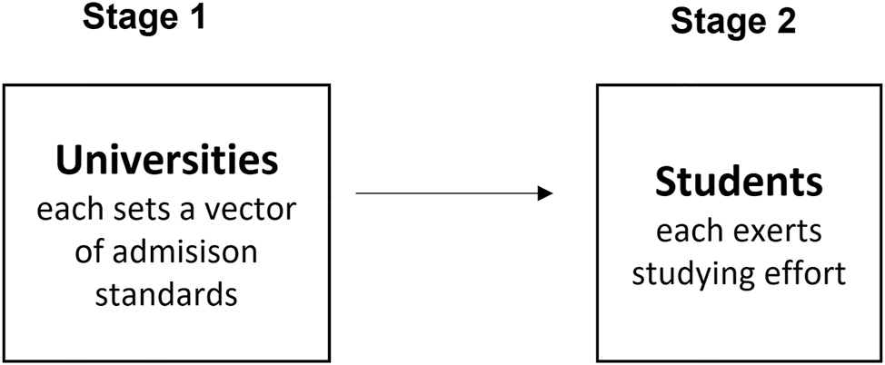
The game between universities and students.

In addition, students know how their peers make their choices, which allows them to form accurate beliefs about the effort of others. Information about these variables becomes crucial for individual students, as universities take them into account when evaluating the effort that a student is perceived to have put into his or her education.

4 Results

4.1 University Ranking

Figure 2 illustrates an example with two universities, u and u′, ranked within the university system U. Suppose f a θ and f d θ are the densities of the universities’ beliefs about the human capital of advantaged and disadvantaged students, respectively. Universities have accurate beliefs about the ability, study effort, and “day of exam” error of these student groups.

Figure 2:

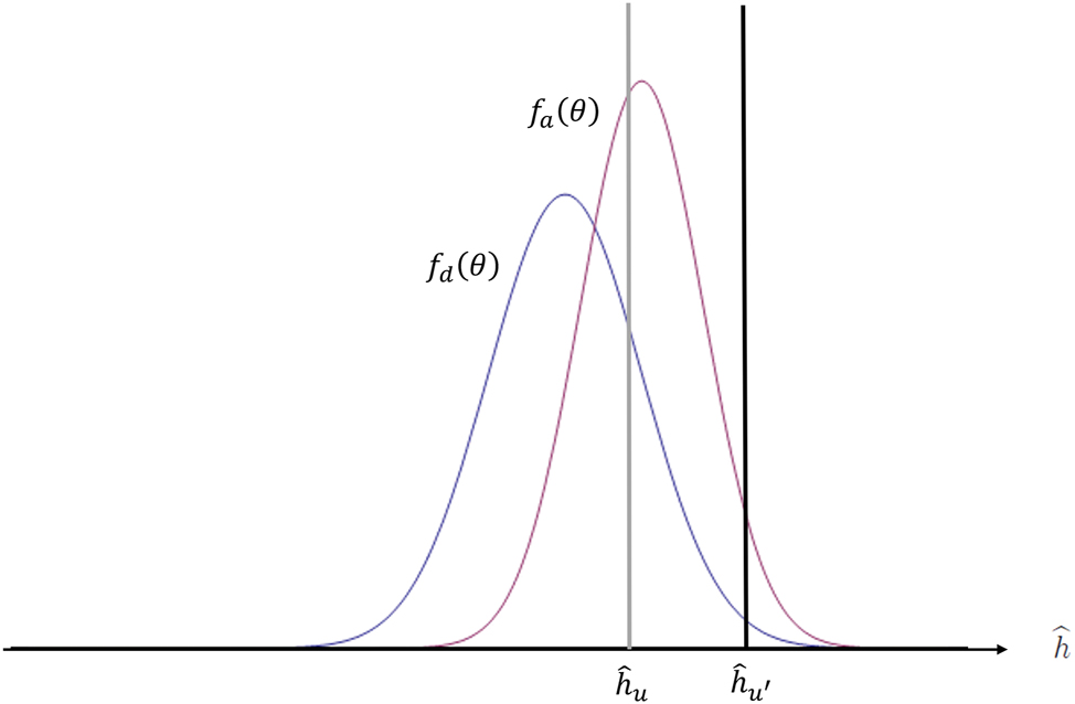
Distribution of expected human capital in the two social groups.

Students from both groups, whose believed human capital exceeds h ̂ u ′ , receive offers from both universities. However, based on their preferences, they choose to enrol in university u′. The interpretation is straightforward: at the end of the school period, a student expects that graduating from a top university will corresponds to a higher chance of getting a higher salary or a better job in the labour market. Subsequently, students whose expected human capital h ̂ lies between h ̂ u and h ̂ u ′ will receive offers from u but not u′, leading them to attend university u. Since we are considering a continuum of perfectly ranked universities, the expected human capital intervals in Figure 2 are infinitesimally small.

In a fully stratified university system, the most prestigious university admits students with the highest expected human capital. The second most prestigious university admits students who fall within the next interval of the distribution of expected human capital, and this stratification continues accordingly down to those students whose human capital is believed to be the lowest in the distribution, who receive an offer only from the university ranked the lowest in the university system.^[16]

4.3 Admission and Social Group

Each university u sets its admission threshold τ u s = τ u d , τ u a based on the level of expected human capital established by its position in the ranking of the university system, h ̂ u . The university system possesses knowledge about the distribution of human capital in each social group, enabling it to determine the functional relationship between a student’s test score within a particular social group and their expected human capital. Additionally, universities are aware of the students’ ranking preferences, which allows them to predict which university each student will choose from those that have extended offers to them. Thus, a student who receives offers from university u but also from any other university positioned higher than u in the ranking of the university system, it will simply enrol in the latter. This implies the following.

Remark 1.

All students enrolled on a certain university exhibit the same level of expected human capital, regardless of their social group. This level of expected human capital corresponds to that below which a university is not willing to admit the student.

We are now in a position to compare the admission criteria for students from different social groups, for given test score. Indeed, Equation (6) represents the relationship between the admission threshold, in terms of expected human capital h ̂ s t of a student from social group s and the test score t. In particular, the relationship depicted by (6) is linear, with slope ρ ε ρ s + ρ ε and intercept, ρ s ρ s + ρ ε θ ̄ s + η e s * . Comparing the slopes of (6), we obtain

ρ ε ρ a + ρ ε < ρ ε ρ d + ρ ε ,

while the difference between the intercepts is ambiguous:

(10) ρ a ρ a + ρ ε θ ̄ a + η e a * ≷ ρ d ρ d + ρ ε θ ̄ d + η e d * .

Substituting the equilibrium efforts from Proposition 1 and rearranging, one gets:

θ ̄ a − g θ ̄ d ≷ η ψ ρ a ρ d − ρ ε 2 ρ a − ρ d ρ ε ρ a ρ d + ρ ε 2 ρ a + ρ ε ,

where g ≡ ρ d ρ a + ρ ε ρ a ρ d + ρ ε < 1 . For the sake of exposition, we denote

Δ θ ̄ ≡ θ ̄ a − g θ ̄ d ∈ R , Φ ≡ η ψ ρ a ρ d − ρ ε 2 ρ a − ρ d ρ ε ρ a ρ d + ρ ε 2 ρ a + ρ ε ∈ R .

Suppose first Δ θ ̄ < Φ , implying that the average ability of students coming from social group d is quite higher than that of students from a ( θ ̄ d > 1 g θ ̄ a ) , and or the precision of the exam outcome is quite lower than that of the distribution of abilities (ρ _ɛ < ρ _d ). This case appears less relevant empirically, but shows that our results do not require any restrictions on the average ability of students coming from different social groups. When Δ θ ̄ < Φ , the expected human capital of d students is systematically higher than that of a students, h ̂ d t > h ̂ a t , because h ̂ a t exhibits a lower slope and a lower intercept than h ̂ d t .

Proposition 2.

If Δ θ ̄ < Φ then, for every university u, students from social group a are admitted with a higher test score than students from social group d:τ _ua > τ _ud .

Figure 3 shows the relationship between all possible test outcomes, on the horizontal line, and the expected human capital required by the highest-ranked university that extends an offer to a student from a given social group with a test score of t. Thus, the dashed line h ̂ a t corresponds to the expected level of human capital for a student from social group a with a test score t, while the solid increasing line h ̂ d t represents the corresponding relationship for students from social group d. The fact that h ̂ d t > h ̂ a t implies that each university requires a higher test score to a than d students. For example, university u requires τ _ud = t′ and τ _ua = t′′, which both signal the same level of human capital h ̂ u τ u = h ̂ d t ′ = h ̂ a t ′ ′ .

Figure 3:

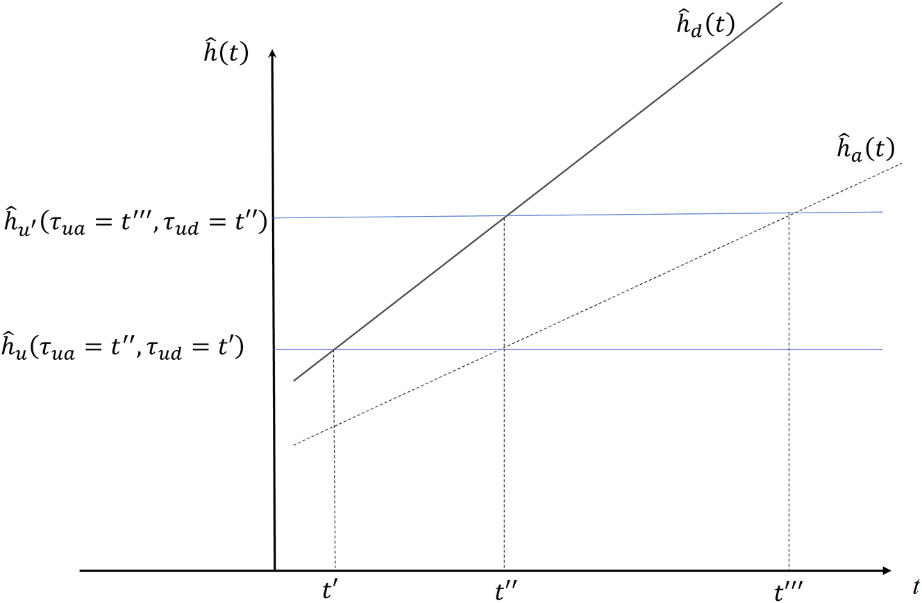
Relationship between the expected university and the test results for students coming from social group d or a: Δ θ ̄ < Φ .

Figure 3 also provides a clear illustration of why students in the group with higher variance exert more effort: a given improvement in the exam result translates into a greater improvement in the most preferred university that makes them an offer than for students from the group with lower variance, and so their incentive to exert effort is stronger.

Next, suppose Δ θ ̄ > Φ , implying that the average ability of a students is sufficiently higher than that of d students. This case is likely more relevant, given the consistent empirical regularity across the world that shows a positive correlation between ability and social background.^[17] From Δ θ ̄ > Φ , it follows that h ̂ a t exhibits higher intercept than h ̂ d t . This in turn implies the existence of a single crossing condition at a certain test result, which we denote as t*.

Lemma 1.

There exists a test outcome t*, such that university u* admits students coming from social groups a and d who got the same test score: τ u * = τ u a * , τ u d * where τ u a * = τ u d * .

The following proposition is a direct consequence of Lemma 1.

Proposition 3.

Each university such that τ ≥ t* admits students from social group a with a higher test score than students from social group d:τ _ua > τ _ud . The opposite applies for each university such that τ < t*.

Figure 4 depicts the relationship between test scores and admitting university, for different social groups, when Δ θ ̄ > Φ . If a student obtained a test score higher than t*, she will enrol in a higher-ranked university if she comes from social group d. In this case, the intuition is the same as in Proposition 2.

Figure 4:

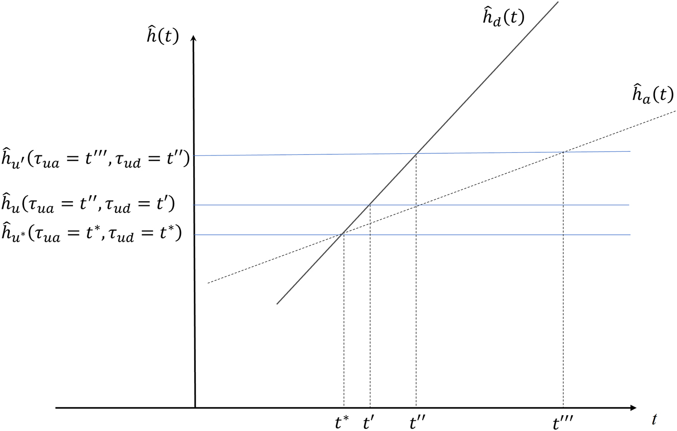
Relationship between the expected university and the test results for students coming from social group d or a: Δ θ ̄ > Φ .

Nonetheless, now the admission criterion of Proposition 2 is confirmed only for universities that expect to admit students with a relatively high human capital. Below a certain threshold t*, a students are expected to have a higher human capital than d students given the same test score. The intuition is simple: when the test score is low (below t*) its weight at explaining the expected human capital is relatively lower than the average ability of the social group. For Δ θ ̄ > Φ , this effect favours a students.

We conclude the section by considering the case with complete information. Now universities observe each student’s ability directly, so that a student’s (known) human capital is:

(11) h i t i = θ i − 1 − η e o * + t i .

In this case, the relationship between test score and university admission strictly depends on the student’s ability level.

5 Anti-Discrimination Policy

In this section, we assume that universities are not permitted to set different admission standards for different social groups. An example of this policy is the so-called “Top 10 % Rule”, implemented in Texas since 1998, which mandates public universities in Texas to ensure automatic admission to all high school seniors who graduate in the top tenth of their class (Niu, Tienda, and Cortes 2006, among others). Our set-up can easily be adapted to this case by adding the additional constraint that τ _us be constant in s.

The first consequence of this restriction is that the test score becomes the sole signal of ability that universities can take into account. From a student’s viewpoint, the expected test score will reflect the level of university where a student i, coming from social group s, expects to be admitted and, as a result, her benefit from attending university, i.e.

where

From a university point of view instead, because a university cannot discriminate based on social groups, the admission results must be the same for each admitted student. Therefore, all students with the same grade will attend the same university level. It follows that the ranking of the university system cannot be based on students’ expected human capital anymore (which would account also for the information of social group) but must rely only on the ranking of test results. Thus, in this case, a monotonic transformation turns test score t into university u.

The second, related consequence is that a student’s expected human capital (6) does not determine which university she will attend anymore:

It follows that students coming from different social groups who obtained the same grade will attend the same university, but their expected human capital differs. In contrast, in the baseline model all students attending the same university had the same expected human capital but different test results.

By substituting (12) into the students’ optimisation problem, we can obtain the result for the case with no discrimination across social groups. Begin by considering students. A student i’s problem becomes

and her optimal choice of effort is given by

where superscript AD stands for “Anti-Discrimination”. Therefore,

Now all students exert the same level of effort. Also, all of them exert higher effort than in the baseline case in which universities can discriminate across students, since the marginal benefit of education is now higher:

for every s.

Next, we turn to the university system. Having already clarified that university admission will follow the level of test scores, we are left to determine the differences in terms of human capital of students by different social groups admitted in the same university.

Students from s admitted in university u have expected human capital

Like in the baseline case, the slope of h ̂ a is always lower than that of h ̂ d . Comparing the intercept of h ̂ a and h ̂ d , we get

Substituting e ^AD from (14) and rearranging, one obtains Δ θ ̄ ≷ Φ A D , where

The case Δ θ ̄ < Φ A D requires that the average ability of d students is much higher than that of a students, i.e.

Even if theoretically admissible, this case is not supported by empirical evidence, and will be left aside to ease the exposition.

Thus, Δ θ ̄ > Φ A D implies the existence of a single-crossing condition between h ̂ a u and h ̂ d u : we denote as u** the university whose students from social groups a and d yield the same level of expected human capital, h ̂ a A D u * * = h ̂ d A D u * * . It follows that

Figure 5 illustrates the relationship between universities and human capital. Unlike the baseline case depicted in Figures 3 and 4, where students were accepted for admission from the same university even with different test results, in this scenario each university of a certain quality requires the same test score for admission. Consequently, students with differing levels of human capital attend the same university. In the example shown in the figure, university u is being attended by students who achieved τ _u : those from social group d have expected human capital h ̂ d u and students from social group a with expected human capital h ̂ a u , where h ̂ d u > h ̂ a u . As the quality of the university increases, so does the difference in human capital between students from different social groups.

Figure 5:

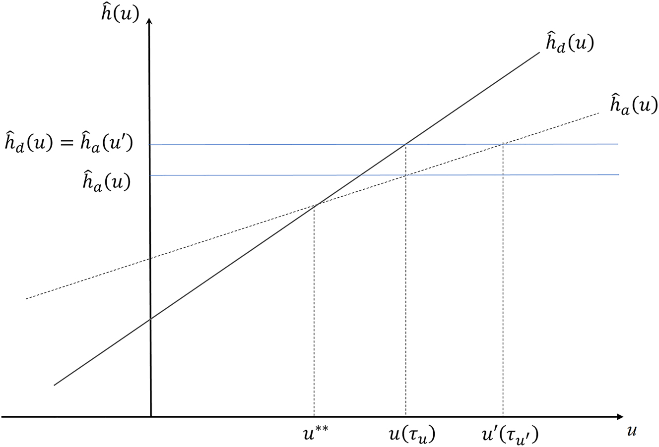
Relationship between human capital and universities when an anti-discrimination policy is implemented.

In terms of policy implications, the direct consequence of Corollary 1 is that, when social groups have different distribution of unobservable ability, the introduction of affirmative action (i.e. lowering the admission threshold for disadvantaged students) would be optimal in terms of admission decisions. Firstly, it allows for the more precise identification of students’ expected human capital, aligning with the university’s objectives. In turn, it narrows down the differences in expected human capital among students from different groups.

However, lowering the admission threshold for students from low social groups below a certain point would effectively reverse the expectation of their human capital. The mixed empirical evidence discussed in the Introduction (Arcidiacono, Aucejo, and Hotz 2016; Melguizo 2008, 2010; Wainer and Melguizo 2018) suggests that our model may indeed provide an interpretation for the potentially different effects of adopting affirmative action policies.

6 Extensions

In this section, we extend our analysis to verify if our results are robust to different assumptions. Firstly, we will assume that the students observe their ability level perfectly. Secondly, we will incorporate university competition, also considering universities with different objectives.

7 Concluding Remarks

In this paper, we have investigated how potentially discriminatory characteristics, such as sex, race, or social background, could influence university admissions. To achieve this, we examined the interaction between students and universities during the admission process. The findings show that higher-ranked universities tend to set lower grade requirements in the admission test for students coming from disadvantaged groups. Conversely, lower-ranked universities follow the opposite pattern. With the implementation of an anti-discrimination policy, students with the same grades will attend universities at the same level. However, they will still exhibit varying levels of human capital based on their social group affiliation.

The results of this study critically rely on the assumption of higher precision of ability in the advantaged social group. While footnote 12 presents a substantial body of empirical evidence, the paper does not directly verify the validity of this assumption through an empirical exercise, which somewhat limits the relevance of the current analysis. Nevertheless, it is reasonable to anticipate a distinct shape in the distribution of ability between students from different social groups. In simpler terms, the slopes of Figure 4 are expected to differ, a priori. A comprehensive empirical investigation to confirm whether disadvantaged students indeed exhibit a more volatile distribution of ability is left for future research.

Finally, our analysis abstracts away from discrimination stemming from bias against members of a specific targeted group (see Becker 1957), which could potentially influence the university selection process in the real world.

The analysis conducted can be adapted to study job recruitment instead of university admission, especially when explaining the role of observable characteristics that may not be relevant to the job. Evidence from field and experimental studies, since Goldin and Rouse’s (2000) seminal work, strongly suggests that if employers are prevented from considering characteristics deemed irrelevant to job performance, their hiring decisions are often significantly altered.^[22] Recruitment services are now proliferating, offering employers protection against discrimination by filtering out all “non-relevant” information provided by job applicants before passing the CV to employers.^[23]

References

Anger, S., and D. D. Schnitzlein. 2017. “Cognitive Skills, Non-Cognitive Skills, and Family Background: Evidence from Sibling Correlations.” Journal of Population Economics 30: 591–620. https://doi.org/10.1007/s00148-016-0625-9.Search in Google Scholar
Arcidiacono, P., and M. Lovenheim. 2016. “Affirmative Action and the Quality-Fit Trade-Off.” Journal of Economic Literature 54: 3–51. https://doi.org/10.1257/jel.54.1.3.Search in Google Scholar
Arcidiacono, P., E. M. Aucejo, and V. J. Hotz. 2016. “University Differences in the Graduation of Minorities in STEM Fields: Evidence from California.” The American Economic Review 106: 525–62. https://doi.org/10.1257/aer.20130626.Search in Google Scholar
Arrow, K. J. 1973. “The Theory of Statistical Discrimination.” In Discrimination in Labor Markets, edited by Ashenfelter, and Rees. Princeton: Princeton University Press.Search in Google Scholar
Aslund, O., and O. N. Skans. 2012. “Do Anonymous Job Application Procedures Level the Playing Field?” Industrial and Labor Relations Review 65: 82–107.10.1177/001979391206500105Search in Google Scholar
BBC News. 2012. “Brazil Approves Affirmative Action Law for Universities.” http://www.bbc.co.uk/news/world-latin-america-19188610.Search in Google Scholar
Becker, G. S. 1957. The Economics of Discrimination. Chicago: University of Chicago Press.Search in Google Scholar
Betts, J. R. 1998. “The Impact of Educational Standards on the Level and Distribution of Earnings.” The American Economic Review 88: 266–75.Search in Google Scholar
Bowen, W. G., and D. Bok. 1998. The Shape of the River: Long-Term Consequences of Considering Race in College and University Admissions. Princeton: Princeton University Press.10.1515/9781400882793Search in Google Scholar
Carneiro, P., and J. J. Heckman. 2003. “Human Capital Policy.” In Inequality in America: What Role for Human Capital Policies? edited by J. J. Heckman, and A. B. Krueger. Cambridge: The MIT Press.Search in Google Scholar
Chadi, A., M. de Pinto, and G. Schultze. 2019. “Young, Gifted and Lazy? The Role of Ability and Labor Market Prospects in Student Effort Decisions.” Economics of Education Review 72: 66–79.10.1016/j.econedurev.2019.04.004Search in Google Scholar
Chan, J., and E. Eyster. 2004. “Does Banning Affirmative Action Harm College Quality?” The American Economic Review 94: 858–72.10.1257/000282803322157124Search in Google Scholar
Coate, S., and G. C. Loury. 1993. “Will Affirmative-Action Policies Eliminate Negative Stereotypes?” The American Economic Review 83: 1220–40.Search in Google Scholar
Costrell, R. M. 1994. “A Simple Model of Educational Standards.” The American Economic Review 84: 956–71.Search in Google Scholar
Cunha, F., J. J. Heckman, L. Lochner, and D. V. Masterov. 2006. “Interpreting the Evidence on Life Cycle Skill Formation.” Handbook of the Economics of Education 1: 697–812.10.1016/S1574-0692(06)01012-9Search in Google Scholar
De Donder, P., and F. Martinez-Mora. 2017. “The Political Economy of Higher Education Admission Standards and Participation Gap.” Journal of Public Economics 154: 1–9. https://doi.org/10.1016/j.jpubeco.2017.07.004.Search in Google Scholar
De Fraja, G. 2001. “Policies: Equity, Efficiency and Voting Equilibrium.” Economic Journal 111: 104–19. https://doi.org/10.1111/1468-0297.00622.Search in Google Scholar
De Fraja, G. 2005. “Reverse Discrimination and Efficiency in Education.” International Economic Review 46: 1009–31. https://doi.org/10.1111/j.1468-2354.2005.00355.x.Search in Google Scholar
De Fraja, G., T. Oliveira, and L. Zanchi. 2010. “Must Try Harder. Evaluating the Role of Effort on Examination Results.” The Review of Economics and Statistics 92: 577–97. https://doi.org/10.1162/rest_a_00013.Search in Google Scholar
De Fraja, G., K. Eleftheriou, and M. Ioakimidis. 2021. “A Note on University Admission Tests: Simple Theory and Empirical Analysis.” The B.E. Journal of Economic Analysis & Policy 22: 623–32. https://doi.org/10.1515/bejeap-2021-0173.Search in Google Scholar
De Groot, M. H. 1970. Optimal Statistical Decisions. New York: McGraw-Hill.Search in Google Scholar
Dewatripont, M., I. Jewitt, and J. Tirole. 1999a. “The Economics of Career Concerns, Part I: Comparing Information Structures.” The Review of Economic Studies 66: 183–98. https://doi.org/10.1111/1467-937x.00084.Search in Google Scholar
Dewatripont, M., I. Jewitt, and J. Tirole. 1999b. “The Economics of Career Concerns, Part II: Application to Missions and Accountability of Government Agencies.” The Review of Economic Studies 66: 199–217. https://doi.org/10.1111/1467-937x.00085.Search in Google Scholar
DfES. 2003. The Future of Higher Education, 5735. Richmond: Department for Education and Skills, HMSO.Search in Google Scholar
Downey, D. B., P. T. von Hippel, and A. B. Beckett. 2004. “Are Schools the Great Equalizer? Cognitive Inequality during the Summer Months and the School Year.” American Sociological Review 69: 613–35, https://doi.org/10.1177/000312240406900501.Search in Google Scholar
Edin, P. A., and J. Lagerström. 2006. Blind Dates: Quasi Experimental Evidence in Discrimination, Vol. 4. Uppsala: Institute for Evaluation of Labour Market and Education Policy.Search in Google Scholar
Epple, D., R. Romano, S. Sarpca, and H. Sieg. 2006. “Profiling in Bargaining Over College Tuition.” Economic Journal 11: 6459–479. https://doi.org/10.1111/j.1468-0297.2006.01132.x.Search in Google Scholar
Epple, D., R. Romano, and H. Sieg. 2008. “Diversity and Affirmative Action in Higher Education.” Journal of Public Economic Theory 10: 475–501. https://doi.org/10.1111/j.1467-9779.2008.00373.x.Search in Google Scholar
Fang, H., and A. Moro. 2011. “Theories of Statistical Discrimination and Affirmative Action: A Survey.” In Handbook of Social Economics, 133–200. The Netherlands: Handbook of Social Economics.10.1016/B978-0-444-53187-2.00005-XSearch in Google Scholar
Flavell, J. H. 1976. “Metacognitive Aspects of Problem Solving.” In The Nature of Intelligence, edited by L. B. Resnick, 231–6. Hillsdale: Erlbaum.10.4324/9781032646527-16Search in Google Scholar
Flavell, J. H. 1979. “Metacognition and Cognitive Monitoring: A New Area of Cognitive–Developmental Inquiry.” American Psychologist 34 (10): 906–11. https://doi.org/10.1037/0003-066x.34.10.906.Search in Google Scholar
Galindo-Rueda, F., and A. Vignoles. 2003. Class Ridden or Meritocratic? An Economic Analysis of Recent Changes in Britain, Vol. 32. London: Centre for the Economics of Education, London School of Economics.10.2139/ssrn.372483Search in Google Scholar
Gary-Bobo, R., and A. Trannoy. 2008. “Efficient Tuition Fees and Examinations.” Journal of the European Economic Association 6: 1211–43. https://doi.org/10.1162/jeea.2008.6.6.1211.Search in Google Scholar
Goldin, C., and C. Rouse. 2000. “Orchestrating Impartiality: The Impact of “Blind” Auditions on Female Musicians.” The American Economic Review 90: 715–41. https://doi.org/10.1257/aer.90.4.715.Search in Google Scholar
Gottschling, J., E. Hahn, C. R. Beam, F. M. Spinath, S. Carroll, and E. Turkheimer. 2019. “Socioeconomic Status Amplifies Genetic Effects in Middle Childhood in a Large German Twin Sample.” Intelligence 72: 20–7. https://doi.org/10.1016/j.intell.2018.11.006.Search in Google Scholar
Hanscombe, K. B., M. Trzaskowski, C. M. A. Haworth, O. S. P. Davis, P. S. Dale, and R. Plomin. 2012. “Socioeconomic Status (SES) and Children’s Intelligence (IQ): In a UK-Representative Sample SES Moderates the Environmental, Not Genetic, Effect on IQ.” PLoS One 7: 1–7. https://doi.org/10.1371/journal.pone.0030320.Search in Google Scholar
Hauser, R. M. 2002. Meritocracy, Cognitive Ability, and the Sources of Occupational Success, Vol. 32. Madison: Center for Demography and Ecology, University of Wisconsin-Madison.Search in Google Scholar
Joshi, H. E., and A. McCulloch. 2001. “Neighbourhood and Family Influences on the Cognitive Ability of Children in the British National Child Development Study.” Social Science & Medicine 53: 579–91. https://doi.org/10.1016/s0277-9536(00)00362-2.Search in Google Scholar
Kaganovich, M., and X. Su. 2019. “College Curriculum, Diverging Selectivity, and Enrollment Expansion.” Economic Theory 67: 1019–50. https://doi.org/10.1007/s00199-018-1109-9.Search in Google Scholar
Krishna, K., and A. Tarasov. 2016. “Affirmative Action: One Size Does Not Fit All.” American Economic Journal: Microeconomics 8: 215–52. https://doi.org/10.1257/mic.20140200.Search in Google Scholar
Lee, V. E., and D. T. Burkam. 2002. “Inequality at the Starting Gate: Social Background Differences.” In Achievement as Children Begin School. Washington: Economic Policy Institute.Search in Google Scholar
Long, M. C. 2004. “College Applications and the Effect of Affirmative Action.” Journal of Econometrics 121: 319342. https://doi.org/10.1016/j.jeconom.2003.10.001.Search in Google Scholar
Lundberg, S. J., and R. Startz. 1983. “Private Discrimination and Social Intervention in Competitive Labor Market.” The American Economic Review 73: 340–7.Search in Google Scholar
MacLeod, W. B., and M. Urquiola. 2015. “Reputation and School Competition.” The American Economic Review 105: 3471–88. https://doi.org/10.1257/aer.20130332.Search in Google Scholar
Marton, F., D. Hounsell, and N. Entwistle. 1997. The Experience of Learning. Edinburgh: Scottish Academic Press.Search in Google Scholar
Mayer, S. E. 1997. What Money Can’t Buy: Family Income and Children’s Life Chances. Cambridge: Harvard University Press.Search in Google Scholar
Melguizo, T. 2008. “Quality Matters: Assessing the Impact of Attending More Selective Institutions on College Completion Rates of Minorities.” Research in Higher Education 49: 214–36. https://doi.org/10.1007/s11162-007-9076-1.Search in Google Scholar
Melguizo, T. 2010. “Are Students of Color More Likely to Graduate from College if they Attend More Selective Institutions? Evidence from a Cohort of Recipients and Nonrecipients of the Gates Millennium Scholarship Program.” Educational Evaluation and Policy Analysis 20: 1–19. https://doi.org/10.3102/0162373710367681.Search in Google Scholar
Metcalfe, J., and A. P. Shimamura. 1994. Metacognition: Knowing about Knowing. Cambridge: MIT Press.10.7551/mitpress/4561.001.0001Search in Google Scholar
New York Times. 2012a. “Rethinking Affirmative Action.” http://www.nytimes.com/2012/10/14/sunday-review/rethinking-affirmative-action.html? Search in Google Scholar
New York Times. 2012b. “Affirmative Action – A Complicated Issue for Asian-Americans.” http://www.nytimes.com/2012/11/04/education/edlife/affirmative-action-a-complicated-issue-for-asian-americans.html? Search in Google Scholar
New York, Times. 2016. “Affirmative Action Isn’t Just a Legal Issue. It’s Also a Historical One.” https://www.nytimes.com/2016/06/25/opinion/affirmative-action-isnt-just-a-legal-issue-its-also-a-historical-one.html.Search in Google Scholar
Niu, S. X., M. Tienda, and K. Cortes. 2006. “College Selectivity and the Texas Top 10% Law.” Economics of Education Review 25: 259–72. https://doi.org/10.1016/j.econedurev.2005.02.006.Search in Google Scholar
Pacelli, K. A. 2011. “Fisher V. University of Texas at Austin: Navigating the Narrows Between Grutter and Parents Involved.” Maine Law Review 63: 569–92.Search in Google Scholar
Phelps, E. 1972. “The Statistical Theory of Racism and Sexism.” The American Economic Review 62: 659–61.Search in Google Scholar
Phillips, M., J. Brooks-Gunn, G. J. Duncan, and P. K. Klebanov. 1998. “Family Background, Parenting Practices, and the Black-White Test Score Gap.” In The Black-White Test Score Gap, edited by Charles Jencks, and Meredith Phillips. Washington: The Brookings Institute.Search in Google Scholar
Reardon, S. 2003. “The Growth of Racial – Ethnic and Socioeconomic Test Score Gaps in Kindergarten and First Grade.” Paper presented at the Annual Conference of the American Sociological Association.Search in Google Scholar
Spence, M. A. 1973. “Job Market Signalling.” Quarterly Journal of Economics 873: 55–74.Search in Google Scholar
Sowell, T. 2004. Affirmative Action Around the World: An Empirical Study. New Haven: Yale University Press.Search in Google Scholar
Wainer, J., and T. Melguizo. 2018. “Inclusion Policies in Higher Education: Evaluation of Student Performance Based on the Enade from 2012 to 2014.” Educação e Pesquisa 44. https://doi.org/10.1590/S1517-9702201612162807.10.1590/s1517-9702201612162807Search in Google Scholar
© 2024 the author(s), published by De Gruyter, Berlin/Boston
This work is licensed under the Creative Commons Attribution 4.0 International License.
Articles in the same Issue
- Frontmatter
- Research Articles
- Asymmetric Performance Evaluation Under Quantity and Price Competition with Managerial Delegation
- Incentive-Induced Social Tie and Subsequent Altruism and Cooperation