Understanding Household Consumption Behaviour: What do we Learn from a Developing Country?
-
Nguyen Van Tran


Abstract
Understanding and changing household consumption behaviour are considered the core driving force of the economic growth of a nation. Vietnam’s economic growth is mainly driven by final household consumption, which constituted over two-thirds of GDP during the last three decades. This paper aims to provide a novel way to understand household consumption decisions in a developing country based on several different but inter-related economic hypotheses of household consumption behaviour. Using a three-wave balance panel dataset constructed from nationally representative Vietnamese household surveys, we find strong evidence to support the importance of the permanent income hypothesis, the life-cycle factor hypothesis and the precautionary savings hypothesis. However, there is no evidence for the sex ratio hypothesis. Addressing the shortcomings of previous studies, this paper confirms the entry and exit of formal sectors and agriculture are the oriental predictors of precautionary motives. Heterogeneity analysis suggests the effect is fairly stable across balance sheet characteristics but varies across consumption categories. Our results are robust to a variety of robustness checks. These findings highlight the importance of combining a wide range of proxies for job insecurity and uncertainty indicators to understand household consumption behaviour, thus providing a powerful test of consumption and savings theories in short panels. The implications of these findings also are discussed and proposed in this research.
1 Introduction and Overview
Vietnamese final household consumption constitutes around 66% of GDP during last three decades, suggesting that restoring consumption levels has become an increasingly important role in fostering economic development. However, the total household consumption rate has declined from 11.76% in 2012 to 7.14% in 2016, which is opposite to the increasing trend of the world average.[1] As a result, understanding how to promote the household consumption rate has caught particular attention among both academia and policymakers. Existing literature suggests understanding its sources in determining consumption-saving behaviour is vital for policy implications[2] and improving welfare.[3] However, although the analysis of household consumption behaviour has become one of the most popular subjects in economic theories (Chai, Rohde, and Silber 2015), the empirical results drawn from the aforementioned studies remain ambiguous.[4] Consequently, debates have emerged in both policy and academic circles about which economic theories are good predictors of household decision-making. To the best of our knowledge, to date, studies on household consumption decisions in developing countries have lagged far behind the developed ones due to limited available resources. Motivated by these facts, this paper contributes to the literature by filling this gap using the nationally representative household panel dataset from Vietnam. The outcomes from this study will contribute to empirical evidence and theories and help policymakers design more appropriate strategies.
Traditional theory of consumption behaviour starts from the life-cycle hypothesis (LCH) by Modigliani and Bumberg (1954), which indicates that income varies systematically over the household’s life-cycle, and households maximise their lifetime utility by saving in a working period. The principal qualification to Friedman’s (1957) permanent income hypothesis (PIH) posits that consumption in a given period is determined by the income over the entire lifetime but not by current income. This framework helps explain the effects of the variation in income and economic shocks on the households’ consumption-savings decisions. Specifically, when households face income uncertainty or risk aversion, their consumption is expected to be lower, as they would expect their permanent income to be reduced in the future. However, the empirical evidence using both micro and macro data is not conclusive (Willassen 1978).
As the traditional models failed to investigate the relationship between expected future income and current consumption and may not adequately capture consumption-saving behaviours, a modern theory generated by Carroll (1994) stated that current consumption solely depends on projected current income and is unrelated to the expected future income. He also showed greater earning uncertainty is associated with lower current consumption. Results are well explained by “buffer stock” models proposed by Deaton (1991) and Carroll (1992, 1997. Prudent consumers might consume more than their current income if they know their future income, whereas income uncertainty in the future results in “buffer stock” saving behaviours. Hence, precautionary savings is considered a buffer stock against uncertainty. The model predicted that prudent consumers will save if the wealth is below the target; thereby, consumption will exceed current income and wealth will increase. A recent branch of literature has introduced and tested the sex ratios hypothesis by Wei and Zhang (2011). A possible explanation is that due to less pressure in the marriage market, households with only female children are more likely to consume more than the others.
Given the central importance of these theoretical results and their effects, it is perhaps not surprising there are sizeable empirical studies focusing on the consumption behaviour in the presence of uncertainty that employed income uncertainty to understand household behaviour (e.g., Miles 1997; Guariglia and Rossi 2002; Dardanoni 1991; Menegatti 2007; Hahm and Steigerwald 1999; Dynan 1993). The other strand used job insecurity and aggregate consumption data (e.g., Guariglia and Kim 2004; Meng 2003; Benito 2006; Stephens, 2004; Carroll, Dynan, and Krane 2003; Lugilde, Bande, and Riveiro 2018; Pericoli and Ventura 2012). The third strand argued that different occupations are associated with different degrees of earning risks; thus, occupations of households are important factors in predicting household decisions (e.g., Fuchs-Schündeln and Schündeln 2005; Skinner 1988; Fisher 1956). In contrast, there is little evidence concerning the simultaneous effects of different but inter-related economic hypotheses of household consumption behaviour in holistic economic modelling. Further, household consumption decisions depend not only on the mean of income uncertainty but also behave differently regarding job mobility (Low, Meghir, and Pistaferri 2010) and adjusting for risk aversion between men and women (Eckel and Grossman 2008). However, the empirical relationship between job mobility and consumption behaviour is limited. Moreover, despite the numerous studies, there is no consensus about the strength of what is an appropriate indicator for job insecurity and uncertainty. This issue must be settled by a comprehensive empirical study.
To address these challenges, the approach used in this research goes beyond existing studies in six main aspects: First, it emphasises the need of a unified framework for consumption hypotheses that can decide household consumption behaviour incorporating a wide range of measurements. Second, unlike previous studies, the unique nationally representative surveys allow us to calculate the propensity of moving in and moving out of occupations, which might be a good indicator for testing the precautionary savings hypothesis. Hence, we pay significant attention to the effect of the propensity for entry and exit of formal occupations and the agricultural sector of individuals on several household consumption categories. Third, although empirical works examine the household consumption response to income insecurity, the aforementioned studies have previously ignored the heterogeneity effects across different household consumption categories and different subgroups. This paper performs the asymmetric effects on different consumption categories. Fourth, due to the nature of taking risk aversion, men and women tend to make different consumption decisions (Eckel and Grossman 2008). However, a key limitation of aforementioned works is they largely ignore the effects of income insecurity on different consumption categories and the nature of taking risks between men and women. Our paper makes an effort to examine precautionary motives of both household heads and spouses in terms of occupations. Fifth, to the best of our knowledge, this is the first attempt to understand what drives different household consumption categories’ behaviour at micro levels in a typical developing country. Finally, while the empirical results could be attributed to different measurement errors or unobserved individuals’ characteristics, the paper’s results are robust to the possibility of various measurements of consumption and econometric techniques.
Under such circumstance, this paper aims to quantify the roles of consumption theories on explaining household consumption behaviour. This is a pioneering effort to represent estimates of consumption functions for households that incorporate all these hypotheses explicitly into a holistic economic modelling. We begin this paper by evaluating permanent and transitory incomes. Following the concept of Musgrove (1979), permanent income is a function of observed individual characteristics. Standard works in macroeconomics obtained permanent income by estimating the effects of current labour income on a set of observable household characteristics (Benito 2006; Fuchs-Schündeln and Schündeln 2005; Guariglia and Kim 2004). Additionally, the permanent income hypothesis (PIH) and its intuition illustrate that consumption should not respond to income fluctuation over time. In other words, consumption is only determined by permanent labour income yet not current labour income, implying the effect of the marginal propensity to consume out of transitory income should be equal to zero. However, recent research in the consumption literature argues that strict conditions could not fit with the real dataset (Meng 2003; Paxson 1992). This would imply that it is important to use the relaxed assumption of the PIH. We extend empirical works by controlling a wide range of household characteristics and accept the weak version of the PIH. Our findings are therefore consistent with the view of the weak version of PIH. Institutively, Vietnamese households are capable of smoothing most categories of consumption over time. This is in line with the findings by Benito (2006), Meng (2003), and Miles (1997), who showed that households are able to even out consumption during difficult periods by savings and borrowings.
Our approach is also new because it contributes to addressing the shortcoming of previous studies in testing one of the most salient risks of the precautionary savings hypothesis. Low, Meghir, and Pistaferri (2010) argued that job mobility is an important indicator to measure employment risk, thus unmeasured job mobility leads to misleading estimates of self-insure and earnings variances reflecting risks. In the dynamic environment, households make labour reallocation decisions across occupations (McCaig and Pavcnik 2015, 2018). Our empirical analysis of precautionary responses to employment risks extends the literature on understanding how the prosperity of employment mobility affects consumption. In our environment, individuals with a riskier income have an incentive to move to other jobs in less risky occupations. We use unique microdata extracted from nationally representative labour force data to evaluate the propensity of individuals to move in and out of formal employment[5] and out of agricultural sectors. Further, the study addresses the concern that people might change their occupations due to their consumption. We had estimated the probability of exit and entry sectors through probit equations. Our results shed some new light on whether switching to lower-risk employment promotes higher consumption. Results confront implications of the precautionary motives. Our affirmative answer indicates that while increasing the predicted probability of moving into formal sectors leads to rising consumption, the opposite is true for the predicted probability of moving out of formal sectors. This implies that moving from informal sectors to formal sectors with lower income insecurity is associated with an increase in consumption.
Another feature of this paper is that Attanasio and Weber (2010) and Paxson (1992) proposed an empirical model to look at life-cycle factors where individuals have concave utility functions. In this field, the objective of this paper is to provide new estimates of how life-cycle factors influence household consumption. Our empirical strategy is to construct a proportion of children, proportion of elderly members and the life-cycle consumption profile of age effects variables to investigate how consumption varies as individuals get older and households with higher numbers of dependent members. We also take care to control for the effect of time and unobserved household characteristics. Wei and Zhang (2011) improved our understanding of household consumption and saving decisions under the unbalanced sex ratio hypothesis. Going beyond that, this paper provides new estimates of the size of households with all sons and households with all females across different consumption categories and different subgroups. Our choice is based on the reason that due to less pressure in the marriage market, households with all females tend to consume more and save less. This paper adds to the work on life-cycle factors and the sex ratio hypothesis by building on appropriate indicators.
Vietnam has unique features and has become an ideal candidate for understanding household consumption behaviour. Our empirical strategy requires the availability of high-quality consumption data at the household level over the period of interest. One of the largest nationally representative surveys is the Vietnam Households Living Standards Surveys (VHLSSs), based on a threewave balanced panel dataset. It is conducted by interviewers and data collected by the General Statistical Office (GSO) of Vietnam with technical assistance supported by the World Bank and the UN Statistics Division, making it ideally suited for this work. With the high-quality data, we are able to look at the changes in consumption over time in the presence of consumption hypotheses controlling unobserved time-invariant individual characteristics and time effects. The second advantage is that the market reform is launched by the Vietnamese government approach, which allowed private entrepreneurs to engage in the market (Migheli 2012). As a result, Vietnamese households are now more likely to face enormous uncertainty due to the dramatic change in socio-economic developments and structural reforms. This evidence raises several questions regarding the main determinants explaining household consumption behaviour. Further, unlike developed countries, although the prevalence of informal employment has been slightly declining—from 62.6% in 2012 to 62% in 2014 and 55.7% in 2016[6]—Vietnam still is characterised by the prevalence of informal employment. Hence, unexpected income shocks should have a significant influence on household consumption decisions.
The results of this paper highlight the importance of simultaneously examining four economic theories with a nationally representative panel dataset across different expenditure categories controlling sample selection biases, other potential bias sources and heterogeneity analysis. More precisely, a 1% increase in the long-run marginal propensity to consume out of permanent income leads to an increase of approximately 0.573% in total household consumption controlling for other theories, fixed effects and unobserved heterogeneity. However, the effect is higher for health expenditure while it is relatively similar for remaining categories of consumption except for the inability to smooth education expenditure. Most remarkably, the results confirm that the validity of the precautionary savings hypothesis heavily depend on the selected proxy of income uncertainty, as already indicated by Stephens (2004). In addition, our results support the argument that household consumption decisions merely depend on the household head characteristics, yet are not influenced by the spouse characteristics. Based on the validation of testing hypotheses, due to being unable to smooth their total consumption over time, the government should support various national savings or borrowing schemes to assist households living without their private households in overcoming negative shocks. At the same time, our findings suggest introducing initial financial supports for the shift of labour out of agriculture and moving out of formal occupations to cope with adverse economic shocks.
The remainder of the paper is organised as follows. The next section presents the theoretical framework. Section 3 presents the data and variables used, Section 4 describes methodology and econometric procedure and Section 5 reports empirical results and discussions. Section 6 discusses asymmetric analysis, Section 7 reports robustness checks, and the last section concludes with policy implications.
2 Theory and Literature
The PIH is the first possible theoretical basis for understanding household consumption behaviour. In the 1950s, Modigliani and Bumberg (1954) introduced the life-cycle hypothesis (LCH), which indicates that income varies systematically over the household’s life-cycle; households maximised their lifetime utility by saving in a working period. The principal qualification to the PIH of Friedman (1957) posits that consumption in a given period is determined by the income over the entire lifetime but not by current income. In other words, consumption depends not only on current income but also on past income and expectations of future income. According to Friedman, consumption does not respond to the changes in total income because permanent and transitory incomes are uncorrelated, and consumption is assumed to be a linear form of income. It is suggested that transitory consumption does not depend on transitory income (earning uncertainty), and the marginal propensity to consume is close to zero. Following the PIH, individuals are able to smooth their consumption by savings in the normal periods or borrowings in the face of transitory fluctuations in income. This framework helps explain the effects of the variation in income and economic shocks on the households’ consumption-savings decisions. Specifically, when families face income uncertainty or risk aversion, their consumption is expected to be lower, as they would expect their permanent income to be reduced in the future. However, the empirical evidence using micro and macro data is not conclusive (Willassen 1978). Therefore, it would be highly desirable to extend this approach to formally test whether households are able to smooth their consumption over their life-cycle.
Second, as the traditional models of the life-cycle/permanent income hypothesis failed to investigate the relationship between expected future income and current consumption, and may not adequately capture consumption-saving behaviours, Carroll (1994) stated that current consumption solely depends on projected current income but is unrelated to the expected future income. He also showed greater earning uncertainty is associated with lower current consumption. Results are well explained by “buffer stock” models, which are proposed by Deaton (1991) and Carroll (1997) and Carroll, Hall, and Zeldes (1992) and Carroll (1997). Prudent consumers might consume more than their current income if they know the future income; whereases income uncertainty in the future results in “buffer stock” saving behaviours, in which precautionary savings are considered buffer stock against uncertainty. The model predicted that prudent consumers would save if their wealth is below the target; thereby, consumption will exceed current income and wealth will increase. Carroll and Samwick (1998) showed this framework is empirically supported by both microeconomic and macroeconomic data. Another theoretical framework emphasises the importance in terms of uncertainty and risk aversion on household consumption. According to Giles and Yoo (2007), the determinants of consumer behaviour are decomposed into three components: the intertemporal substitution effect, the life-cycle effect and the precautionary saving effect. It can be predicted that the expected future variance of consumption shocks has a positive effect on consumption growth in the future because of an increase in saving rate.
This theoretical result has been empirically investigated by numerous papers. Given the magnitude and importance roles of household consumption on economic growth, identifying core factors driving household consumption has become one of the most popular topics recently (Chai, Rohde, and Silber 2015). However, most previous studies in this area have been motivated to examine the effects of income uncertainty on household consumption by considering the precautionary saving hypothesis. There are three main strands of literature. The first strand, which has attracted the attention of most researchers, directly measures income uncertainty from households’ incomes. Miles (1997) and Guariglia and Rossi (2002), measuring uncertainty by the residuals from earning equations, found a strong precautionary saving motive in Britain and the UK. Similarly, in support of precautionary savings hypothesis, Dardanoni (1991) and Menegatti (2007) approximated income uncertainty by the variance of labour income in the UK and Italy, respectively, and Hahm and Steigerwald (1999) measured uncertainty through the conditional standard deviation of income in the US. However, Dynan (1993), measuring uncertainty by the instrument variables of the variance of income change in the US, argued that precautionary saving motives fail to predict household consumption behaviour. However, these analyses face significant measurement and methodology issues, particularly regarding the quality of income uncertainty data. The second strand of literature, which used job insecurity as a proxy for individual uncertainty, produced contradictory results. Using the probability of job loss to measure income uncertainty in Russia, Guariglia and Kim (2004) found evidence of precautionary saving motives. In addition, Meng (2003), using data on China, found the predicted probability of being unemployed negatively affects household expenditure. However, using both unemployment risks and the predicted probability of job loss in Britain to measure uncertainty, Benito (2006) obtained different conclusions: while unemployment risks do not impact household consumption, increasing the predicted probability of job loss decreases consumption.
Conversely, measuring uncertainty by expectations of future job loss, Stephens (2004) concluded that precautionary saving motives do not exist in the US, while using job loss shows contradicting conclusions. Carroll, Dynan, and Krane (2003) tested the precautionary saving hypothesis in the US and found little evidence to support this hypothesis. Further, Lugilde, Bande, and Riveiro (2018), using different sources of uncertainty, showed the magnitude sign effects of uncertainty on household consumption heavily depend on the selected proxy of income uncertainty. Producing an alternative measurement of uncertainty in Italy, Pericoli and Ventura (2012) found the probability of marital splitting has powerful and negative effects on current consumption, which supports the precautionary saving motives. However, attempts to test the precautionary hypothesis have met with mixed findings.
Additionally, occupations of households are essential factors in predicting household decisions. Different occupations are associated with different degrees of earning risks. Hence, people with risker occupations might save more and consume less. For example, individuals who work for governments as civil servants might consume more and save less than others because the former face lower job uncertainty and have long-term contracts. To support this, Fuchs-Schündeln and Schündeln (2005) found that civil servants, who have low-risk occupations, have significantly lower financial wealth than non-civil servants with higher risk aversion in Germany and confirmed the existence of precautionary savings. Additionally, Skinner (1988), empirically examining the importance of precautionary savings based on different occupations of household’s head as a proxy of uncertain earning in the US, found that service workers and labourers have low average saving rates, suggesting the lower degree of earning risks lead to low average saving rates. These results are consistent with the precautionary saving hypothesis. However, while Fisher (1956) concluded that managers saved 12% less than self-employed people, Skinner (1988) showed farmers and the self-employed likely had low saving rates. One of the potential problems is the selection of occupations. Individuals with more risky occupations have an incentive to move to other jobs in less risky occupations. Our empirical approach attempts to avoid the potentially biased selection of occupations by considering different types of occupations. More precisely, we consider different behaviour between households that have a member working as civil servants and others because this type of job will be selected by governments. The paper also calculates the probability of entry or exit of formal occupations.
Overall, the previous attempts to test the precaution saving hypothesis related to consumption mainly concentrated on developed countries and produced mixed or inconclusive conclusions. Additionally, due to the nature of taking risk aversion and different personality traits, men and women tend to make different consumption decisions (Eckel and Grossman 2008; Mangiavacchi, Piccoli, and Rapallini 2021). However, previous empirical studies have ignored whether women with lower occupational risks are more likely to consume more than those with higher risks. Our paper makes an effort to examine the precautionary motives of both household heads and spouses in terms of occupations.
Another predictor of household consumption behaviour is life-cycle factors. Parents are expected to receive support from their children as they get older or retire; thus, they would be willing to invest more in their children (Paxson 1992). This is also confirmed by the fact that almost elderly people choose to live with their family when they retire. For life-cycle patterns, the nexus between consumption, income and age follows an inverted U-shape or a hump shape, whereby both consumption and income increase during the first part of the life-cycle profiles, then reach a peak before decreasing as people get older. This explanation does not appear to align with the life-cycle profiles, where Attanasio and Weber (2010) showed that both income and consumption would become much flatter as households become older. Considering the importance of life-cycle factors in explaining household decisions, the higher number of children and elderly people are expected to negatively impact consumption, according to Paxson (1992). It has been posited that the age of individuals’ variables is a more powerful predictors in understanding consumers’ decisions. Attanasio and Weber (2010) utilised the life-cycle model to explain that individuals have concave utility functions, and therefore only unanticipated permanent income changes cause a change in consumption. They also provided strong evidence that there is an invested U-shape relationship between the age of the household head and consumption and income. This was also found by Fernández-Villaverde and Krueger (2007) and Gourinchas and Parker (2002), yet a contradicting result is found by Gertler, Levine, and Moretti (2009).
Finally, a recent branch of literature has generalised the importance of the sex ratio hypothesis. Differing from traditional predictors of household consumption and savings decisions, Wei and Zhang (2011) introduced and tested the sex ratios hypothesis. Specifically, to take comparative advantage in the marriage market, Chinese parents with a son need to accumulate assets to improve their chance of their child getting married. Therefore, a possible explanation is that due to less pressure in the marriage market, households with only female children are more likely to consume more than others. In addition, Vietnam is one of the East Asian countries in which the roles of family members are clearly defined due to social norms, whereby parents have a social responsibility to take care of their children and elderly members. Hence, a household with more children or elderly people is more likely to consume more and save less. The shortage of females in Vietnam would have resulted from the government’s population policy, known as a one-or-two child policy established in 1989. Therefore, sex-selective abortions are a problem in Vietnam (Bélanger and Oanh 2009). Similar to China, households with all sons are more likely to consume less and save more to have an advantage in the marriage market. Conversely, after getting married, a woman tends to move to live with her husband’s family to take care of elderly people, as sons are expected to take responsibility and care for their parents in old age as a social norm. Therefore, households with all female children tend to save more and consume less to smooth their consumption in their older age. All these characteristics make Vietnam a unique and interesting subject to explore. Our expectation is that households with all female children are more likely to consume more than those with all male children.
By summarising all the discussions above, it can be seen that household consumption behaviour might be predicted by a variety of consumption theories, which mainly forces on precautionary saving motivations, PIH, life-cycle factors and the sex ratio hypothesis. Our empirical study relies heavily on theoretical predictions of the consumption-savings decisions. In the concept of precautionary savings, the economic theory predicts that households with precautionary motives will consume more when future income uncertainty is lower. Hence, to empirically estimate the effects of income uncertainty on consumption decisions, it is important to know how to measure uncertainty. According to the standard Euler equation, the variance of consumption shocks as a proxy of uncertainty is related to the expected consumption growth. However, Hahm and Steigerwald (1999) argued the sign of the coefficient in the Euler equation is unclear. In this paper, besides the job loss in the next 12 months, we propose the alternative indicators of occupational insecurity, which is the most important source of income uncertainty. This suggests households might postpone their consumption when they work in high-risk occupations. Besides, the permanent income hypothesis predicts that consumption in a given period is not determined by income in that period (transitory income) but by income over their entire lifetime (permanent income). Additionally, the sex ratio hypothesis is another predictor of household consumption decisions, requiring further explanation since it is rare in Vietnam. Finally, the life-cycle factors hypothesis attaches significant importance to predicting household decisions, since different countries with different cultural and social norms might consume more or less. Considering these hypotheses, a hypothesis framework incorporated with factors affecting household consumption decisions is displayed in Figure 1. However, the effects of different indicators based on different theories maybe not be obvious and need further confirmation.
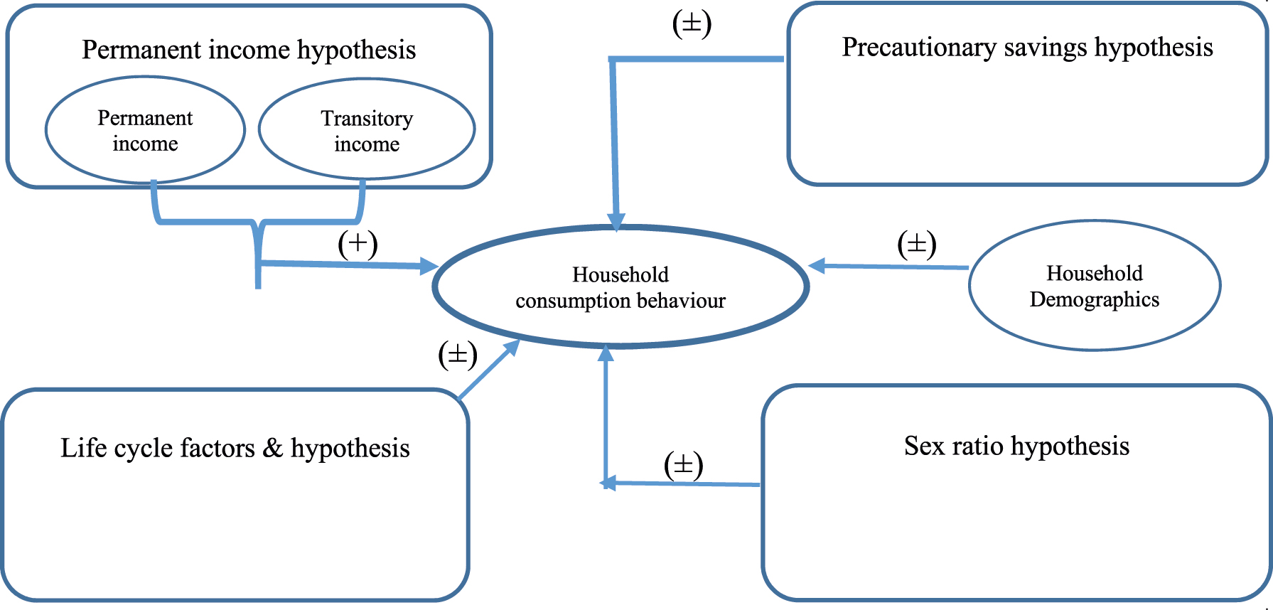
The hypothesis framework of household consumption behaviour.
3 Data Description and Variables Used
3.1 Data Sources
In this research, we use the VHLSSs, a national household survey conducted by Vietnam’s General Statistics Office with technical support from the World Bank. The nationwide surveys were designed to be significantly representative, both at core module topics and national levels. The dataset contains a wide range of information on the living standards of all social societies that can be used to obtain nationally representative summary statistics. However, it should be noted that while the survey consists of detailed information on household consumption categories, it does not collect information related to individuals’ consumption. Therefore, it is reliable to evaluate the impact of earning uncertainty on consumption at household levels. From 2002, the national survey has been carried out every two years. Households were interviewed bi-annually with various questions regarding ages, genders, educational levels, income sources, consumption categories, assets, health, and remittance both in domestic and international sources.
This paper uses the largest sample size of cross-sectional household surveys in 2016, 2014 and 2012. The sample size for the VHLSS 2012, the VHLSS 2014, and the VHLSS 2016 is 9399 households from 3130 communes. For each year, we have cross-section data of households. We also construct balanced panel data to have a comprehensive view of whether the relationship between consumption and income uncertainty has changed over time. The sample starts from 2012, which has a higher sample size but there are no government policy interventions during these periods. These surveys contain rich information on household consumption categories because of their comprehensive measure of household consumption expenditures and the wide range of socio-economic backgrounds of households. Further, using micro data set allows us to directly test whether households facing income uncertainty behave following the theoretical prediction in terms of changing their consumption. To overcome sample selection bias in sample selection, we consider labour force participants and thus exclude households where the household head’s age exceeded 60 years old or retired if they are male and 55 years old if they are female, in accordance with labour laws in Vietnam. We also exclude households in which all members are elderly people or children. The families with a negative total income, which might come from measurement errors, are also eliminated from our analysis. We use balanced panel data from 2012 to 2016 for a comprehensive view. It is emphasised that 50% of households will be interviewed in the next round. Therefore, we will have around 2500 households interviewed in 2012, 2014 and 2016.
3.2 Measurement of Variables and Data Description
3.2.1 Household Consumption
First, our measure of household consumption is obtained directly from the total household expenditure of all goods and services. However, evidence from previous studies (e.g., Dynan (1993) for non-durable and services consumption; Stephens (2004) for total household expenditure; Meng (2003) for total household expenditure, food consumption and educational expenditure; Guariglia and Rossi (2002) for food and groceries; and Lugilde et al. (2018) for non-durable goods) indicates that changes in durable goods consumption or food consumption do not closely relate to change in total consumption. Therefore, we also categorise total household purchases into a wide range of household expenditures to explain the income uncertainty effects on particular expenditures, such as non-durable goods consumption and durable goods expenditure, education expenditure, health expenditure, food consumption and non-food consumption. The paper uses household consumption rather than household income data for two appropriate reasons: (1) because the purpose of this study is to examine how economic theories work in explaining household consumption behaviour; and (2) data on household consumption is often easier to obtain than income data as there are many inherent problems calculating and defining household income in developing countries like Vietnam. For example, it is difficult to measure income from self-employed workers in agriculture and aquaculture, where a large proportion of labour participation is taken into account. Considering the potential non-normality of household consumption categories and heteroskedasticity, all variables were transferred to natural logarithms in the regression.
3.2.2 Precautionary Motives
Job loss represents one of the most important sources of uncertainty that households face. We used both household head and spouse not working by the self-reported unemployment responses for 12 months. However, it is only an indicator that captures the true employment status of main household earners. The second measurement affecting precautionary motives as occupational indicators follows and extends the approach of Fuchs-Schündeln and Schündeln (2005), Lugilde, Bande, and Riveiro (2018), and Skinner (1988). This is because different occupations are significantly associated with different degrees of earning risks. Regarding different occupations, manual labour and low-skilled workers have the highest income uncertainty compared with the other occupations. Waged employees have the lowest income uncertainty followed by self-employment in agriculture and self-engagement in the non-agriculture sectors. Further, civil servants, who face the lowest income risk compared to other jobs have significantly higher consumption than households in other occupations. Besides, to have better occupational indicators, we added not only a variety of occupations of the household head but also included the occupations of spouses due to the natural difference of taking risk aversion between males and females. Unlike previous studies, the unique nationally representative surveys allow us to calculate the propensity of moving in and out of occupations, which might be a good indicator for testing the precautionary savings hypothesis. In our environment, individuals with a riskier income have an incentive to move to other jobs in less risky occupations. Hence, we pay significant attention to the effect of the propensity for entry and exit of formal occupations and agricultural sector individuals on several household consumption categories.
3.2.3 Permanent Income and Transitory Income
The predicted values represented permanent income from the household income equation, where the household income equation is a function of demographic and social-economic characteristics of households. Then, the difference between the actual household income and permanent income is transitory income. Notably, we used the weak version of PIH in our empirical findings.
3.2.4 Life-Cycle Factors
As previous mentioned, the proportion of children and proportion of elderly people were used in this research, which is considered a situation of uncertainty regarding life span, as parents are more likely to invest in their children as the means of accumulating their expected future assets. Additionally, this paper mainly used the age of household head and age squared of household head to examine the LCH. Although examining the LCH can use many forms of age-specific relationships influencing individuals’ behaviour, as expected, our present interest focuses on the negative sign of the square of the age of the head of household variable.
3.2.5 Sex Ratio Indicators
Wei and Zhang (2011) stated that with less pressure in the marriage market, households with only female children are likely to consume more and save less. Following their approach, we used two dummy variables—households with all female children and households with all male children—as a proxy for the sex ratio hypothesis. Our explanation is that families with all females are likely to consume more than others.
3.2.6 Control Variables
To investigate the effects of income uncertainty on household consumption in Vietnam, we followed, extended and developed empirical modelling from Benito (2006) in Britain, Lugilde, Bande, and Riveiro (2018) in Spain, Miles (1997) in the UK and Meng (2003) in China by incorporating a series of potential determinants. The following control variables are used: health insurance of household head and home ownership, household assets, living areas, and number of years of schooling. The reasonable selection of variables in this research is based on a wide range of empirical studies that we consider potential control variables, which influence household consumption behaviour.
The information on the data description across different samples is shown in Table 1. Following Figure 1, Table 1 provides summary data from Vietnamese surveys of the different consumption categories and households’ characteristics for a balanced panel data running from 2012 to 2016. It is noted that all numbers in the table are in thousand VND. As seen from the table, the average amount of total household consumption expenditure was 84506.44 thousand VND. In terms of the life-cycle factor, Figure 2 shows that when the household head gets older, both income and consumption grow smoothly. Further, while income and consumption of households have more fluctuations in 2016 when people get older, these trends gradually increase as household heads get older. All household consumption categories and income of households are relatively stable at the end of retired ages.
Summary statistics for characteristics of the Vietnamese households.
| Indicator | Variable type | Mean | Std. |
|---|---|---|---|
| Total consumption | Cont | 84,506.44 | 73,209.99 |
| Durable goods | Cont | 23,861.55 | 31,324.37 |
| Non-durable goods | Cont | 60,644.88 | 54,488.96 |
| Food consumption | Cont | 48,814.33 | 47,277.34 |
| Non_food consumption | Cont | 35,692.11 | 39,079.43 |
| Occupation position of household head | Ordinal | 2.7001 | 0.4957 |
| Occupational situation of household head | Ordinal | 2.7399 | 1.2038 |
| Employment status of head of household | Binary | 0.0687 | 0.2529 |
| Working in economic sectors of household head | Ordinal | 3.0979 | 0.9534 |
| Household head being not working | Binary | 0.9637 | 0.1871 |
| Occupation position of spouse | Ordinal | 2.7126 | 0.4625 |
| Occupational situation of spouse | Ordinal | 2.8122 | 1.1277 |
| Employment status of spouse of household | Binary | 0.0613 | 0.2399 |
| Working in economic sectors of spouse | Ordinal | 3.3980 | 0.8243 |
| Spouse of household being not working | Binary | 0.8372 | 0.3693 |
| Proportion of children | Cont | 47.1773 | 49.2792 |
| Proportion of elderly | Cont | 3.8691 | 14.4926 |
| Household with all sons | Binary | 0.2709 | 0.4445 |
| Household with all daughters | Binary | 0.1892 | 0.3917 |
| Household income | Cont | 13,9222.1 | 12,8086.1 |
| Household asset | Cont | 39,117.43 | 90,158.75 |
| Age of household head | Cont | 44.2806 | 8.3904 |
| Family size | Cont | 4.0000 | 1.3449 |
| Ethnicity | Binary | 0.7852 | 0.4107 |
| Gender | Binary | 0.8638 | 0.34302 |
| Proportion of unhealthy | Cont | 29.5108 | 57.3660 |
| Marriage status | Binary | 0.9055 | 0.2925 |
| Location | Binary | 0.2916 | 0.4546 |
| Number of years schooling | Cont | 7.6428 | 3.5159 |
| Educational levels of household head | Ordinal | 3.3753 | 1.1490 |
| Home ownership | Binary | 0.9756 | 0.1543 |
| Living area | Cont | 81.2789 | 49.2960 |
| Poor | Binary | 0.1197 | 0.3247 |
| Educational levels of spouse | Ordinal | 3.2999 | 1.4367 |
| Health insurance | Binary | 0.5875 | 0.4924 |
| Red river delta | Binary | 0.1940 | 0.3955 |
| Northern midlands and mountainous | Binary | 0.2306 | 0.4213 |
| North Central Coast | Binary | 0.1038 | 0.3051 |
| South Central Coast | Binary | 0.1140 | 0.3179 |
| South East | Binary | 0.0953 | 0.2937 |
| Mekong river delta | Binary | 0.1787 | 0.3832 |
| No. Obs | 3525 |
-
Using GDP deflator from World Bank Indicators to obtain real consumption and income in panel data with 2012 being the base year, all data are calculated from the VHLSSs 2012, 2014 and 2016.
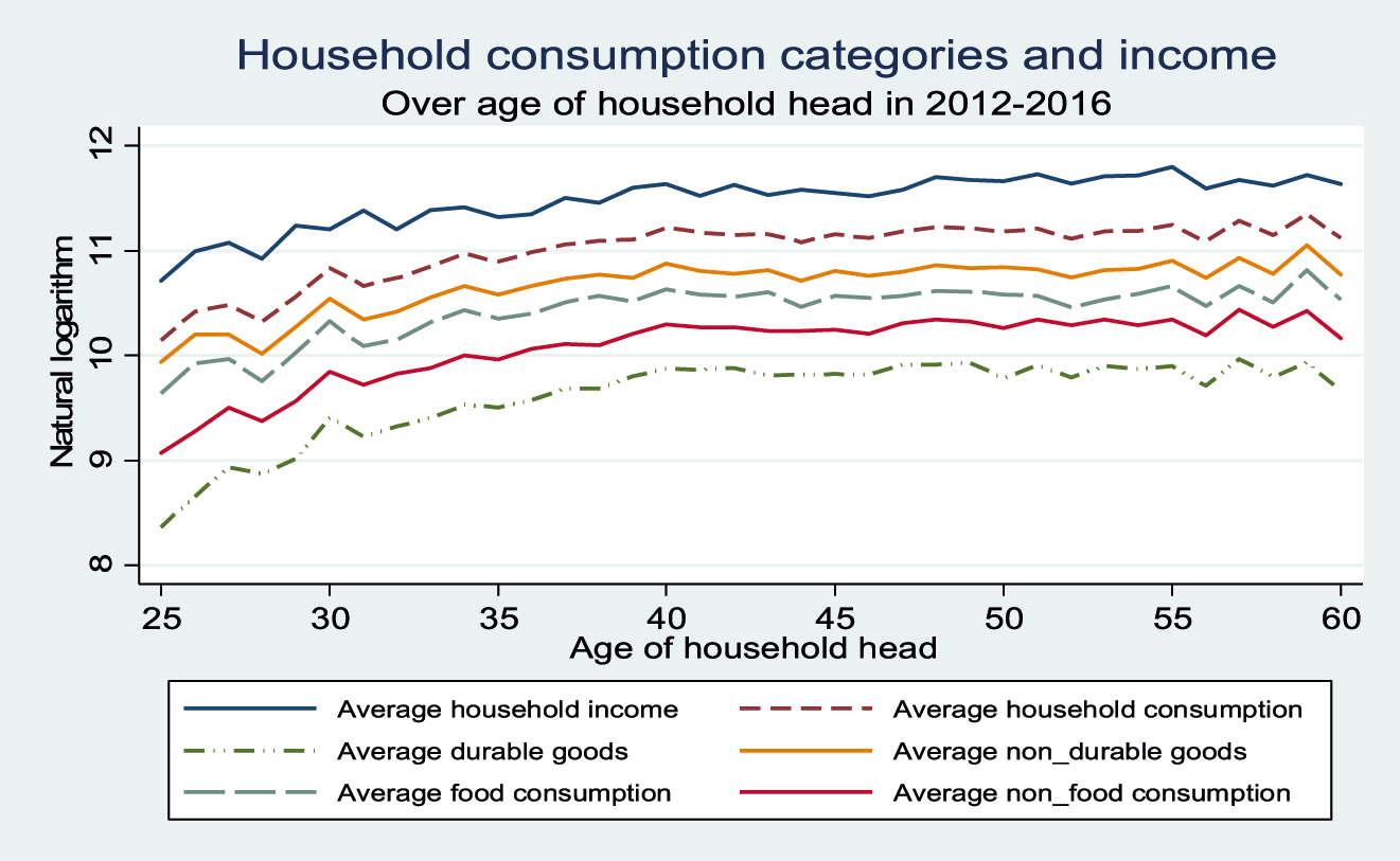
Household consumption and income over age of household head in 2012–2016.
Additionally, there is relatively no difference between male and female household heads in terms of average consumption categories and income, as shown in Figure 3. This finding is not surprising because females and males have a similar ability to manage their household’s expenditures, ceteris paribus. Figures 4 and 5 present the difference in household consumption expenditures and income across ethnicity and location, respectively. It appears that households living in urban areas and Kinh ethnicity are wealthier than those living in rural areas and minority ethnicities. Therefore, their expenditures in terms of durable goods, non-durable goods, and food and non-food items are much higher. This is consistent with the supposition that people in cities might have many opportunities to obtain high-wage work, while living costs in urban areas are higher than in rural areas.
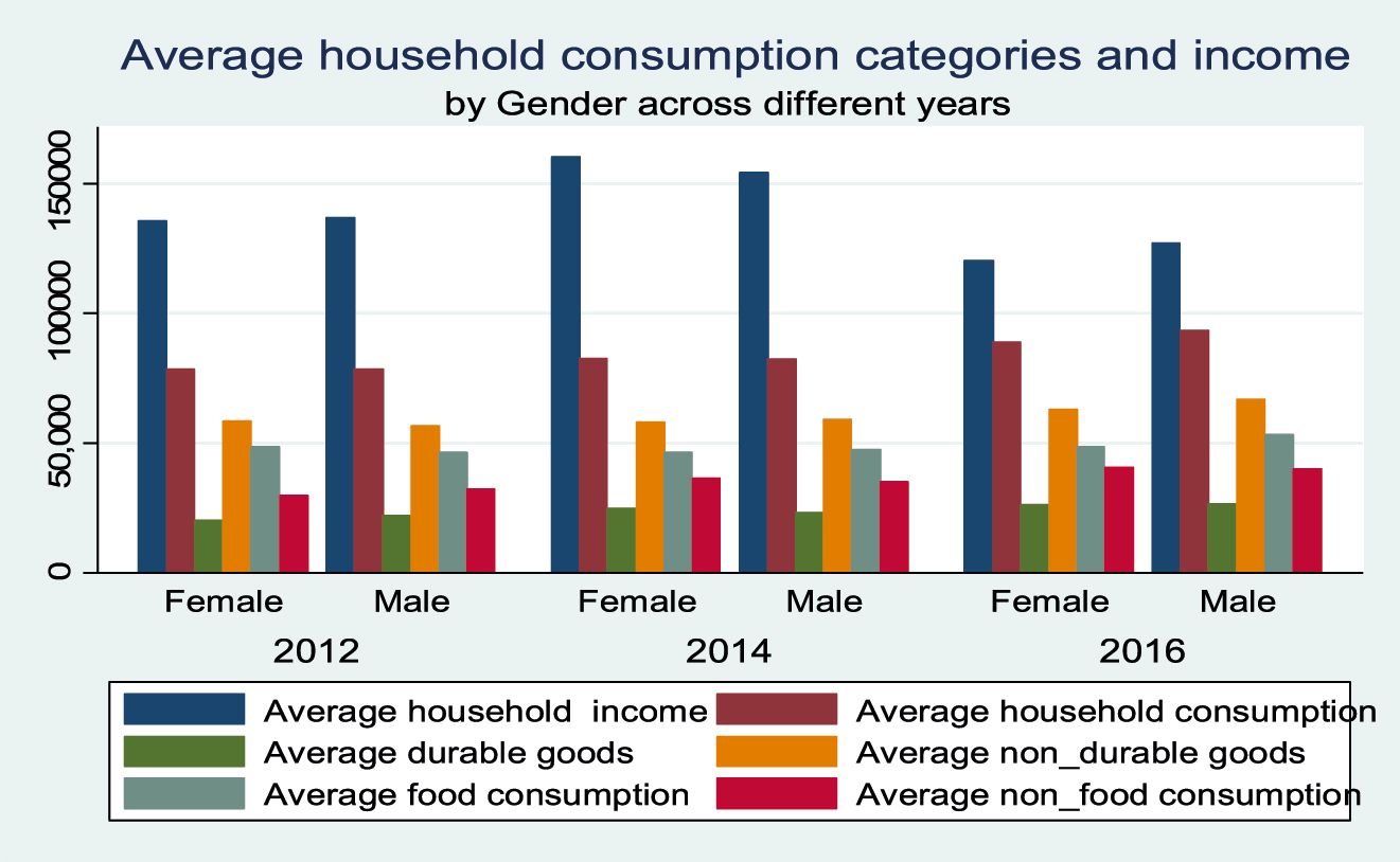
Household consumption and income by gender of household head.
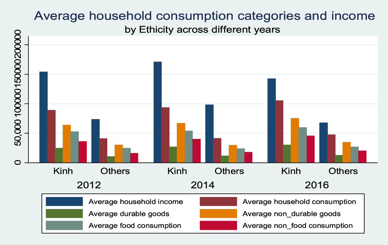
Household consumption and income by ethnicity of household head.
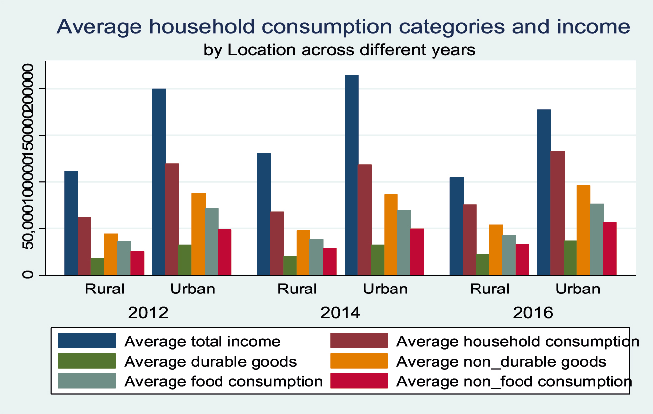
Household consumption and income by location of household head.
Of course, this evidence does not necessarily imply that households living in urban areas and Kinh peoples are at a higher risk in terms of occupations and greater income uncertainty. Indeed, the increase in household consumption is matched by a parallel increase in household income over the age of the household head, which could be supported by the LCH.
4 Econometric Modelling and Estimation Procedure
Based on the variables discussed in the previous section, the following model in Eq. (1) sets up the econometric model using micro balanced panel data of three waves for households in Vietnam. The aim is to unify the model and study four hypotheses simultaneously to evaluate how four factors can explain household consumption decisions. Therefore, the discussion so far implies the following fixed effects regression can be written as:
where CONSUMP
it
is the outcome of interest, and the natural logarithm of household consumption by household i of year t; X
it
includes a wide set of household-specific characteristics such as regions, household assets and household head educational levels, which are assumed to significant influence on consumer behaviour;
The expression allows us to test several hypotheses, including the PIH, the LCH, the sex ratio hypothesis and precautionary saving hypothesis. Notably, the PIH and its intuition suggested that consumption should not respond to income fluctuation or consumption is only determined by permanent labour income but not current labour income, implying the marginal propensity to consume of transitory income should be equal to zero (β2 = 0) while its permanent income is 1 (β1 = 1). However, the empirical evidence argues that these strict conditions do not fit with the real data due to income uncertainty and borrowing constraints (Meng 2003; Paxson 1992). As a result, the life-cycle or permanent income hypothesis was rejected (Souleles 1999). Hence, the relaxed assumption of PIH should be applied, which is β1 > β2 (Meng 2003; Miles 1997). In this specification of consumption modelling, W it represents the life-cycle factors indicate that households with more children and more elderly people are expected to save less and consume more (Paxson 1992). Another explanation is that parents are expected to receive support from their children when they get older or retire, so they will spend more on their children as an investment in their life. It is also true that almost all elderly people choose to live with their families when they retire. In East Asian countries, the roles of family members are clearly defined due to social norms. Parents are expected to have a social responsibility to take care of children and elderly members. Therefore, households with more children also spend more and even save less. It is suggested that the sign of γ is expected to be positive correlation with consumption.
Additionally, according to the life-cycle theory, the relationship between age and total consumption exerts the invested U-shape curve as the well-known concave age-consumption nexus. Hence, we expected the signs of the coefficient of the age variable and the age square variable are significantly positive and negative, respectively. Further, based on the precautionary saving hypothesis, if Vietnamese households are precautionary savers, the signs of θ1 and θ2 should be significantly negative. And τ1 and τ2 should be significantly positive signs if the occupations with low labour income risk have significantly higher consumption in comparison with other occupations. For multiple choices of occupations, it is expected that the consumption of lower-risk occupations is likely higher than that of higher risk ones. As mentioned before, due to less pressure in the marriage market, a household with all female children (F it ) is more likely to consume more than households with all male children (M it ). The alternative explanation is that a woman tends to move to live with a man’s family after marriage. In other words, families with only female children might consume more.
Our key regressors are the earning uncertainty of both head and partner households for the precautionary saving hypothesis, households with all female children or male children for the sex ratio hypothesis, and the proportion of children and elderly members and the age variable for life-cycle factors. To test the existence of the precautionary saving hypothesis by evaluating the impact of household income uncertainty on the current consumption as H0 : θ i = 0 and H1 : θ i < 0, because in the presence of income uncertainty, it is optimal to reduce the current consumption. The other test is H0 : τ i = 0 and H1 : τ i > 0, to indicate that individuals with low-income risk occupations have significantly higher current consumption than others with high labour income risk and vice versa. Besides, we assess the existence of PIH, sex ratio hypothesis and LCH regarding the coefficients of γ, φ, β1 and β2.
Several econometric issues should be addressed. An important potential bias in the estimated effects of income uncertainty is the current consumption function does not include all relevant factors affecting household consumption, such as household tastes or wealth. Therefore, the error term might correlate with proxies of income uncertainty and income. However, the purpose of this study is to estimate the effect of proxies of income uncertainty on consumption, not labour income. In this case, we assumed that income variables are exogenous. Miles (1997) showed that human capital accumulation is an important source of income and consumption; thus, income might be correlated with the error term in Eq. (1), whereas it is beyond our scope. Hopefully, it will be accounted for the future research. Another potential problem is individuals prefer to switch in low-risk types rather than high-risk types due to risk aversion influences; therefore, the empirical results might be inconsistent because of the unobserved risk. To overcome this issue, we provide empirical results that include and exclude farmers and self-employed households. By doing this, the endogeneity and the selection bias could be eliminated. To correct for heteroskedasticity, the paper uses White’s heteroskedasticity consistent standard errors to adjust for potential heteroskedasticity.
One of the potential problems is the selection of occupations. Individuals with a riskier income have an incentive to move to other jobs in less risky occupations. Our empirical approach attempts to avoid the potentially biased selection of occupations though considering the different types of occupations. More precisely, we consider different behaviours between households that have a member working as civil servants and others because this type of job will be selected by governments. Additionally, there are many constraints to prevent individuals from changing their occupations in around four years (2012–2016); thus, we calculate the probability of entering and exiting formal occupations and moving out of the agriculture sector.
Estimating the consumption function in Eq. (1) requires information on both permanent and transitory labour incomes, in which permanent income is the income that a household would earn without idiosyncratic shock, while transitory labour income is defined as the difference between current incomes and permanent incomes. According to Musgrove (1979), permanent income is a function of observable variables, which is represented by a matrix X and an error term ɛ as follows:
Therefore, our research follows this way when estimating permanent labour income with the micro balanced panel dataset from 2012 to 2016. We extend Fuchs-Schündeln and Schündeln (2005), who used instrument variables for obtaining permanent income through a household’s characteristics. We also followed Benito (2006) and Guariglia and Kim (2004) to obtain the predicted values as a proxy of permanent labour income by estimating the effects of variables from a set of observable household characteristics on a log of labour income of households by random effects. That is because the permanent income can be expressed by the equation to capture age cohort effects and non-homotheticity of preferences. Notably, the error term ɛ might contain unobserved individual characteristics that are also accounted for in permanent income (Bhalla 1980) when using cross-sectional data.[7] They also suggested that an alternative approach using cross-sectional data is the weighted average of incomes to calculate permanent income. However, to apply this, it is necessary to have past income data (Meng 2003). Unfortunately, we do not have such information on households’ previous incomes. Therefore, to obtain more precise results, we calculated the predicted values from the income equation as an appropriate indicator of permanent income by using a random effects regression. We control a wide range of household characteristics in earning equations in a balanced panel data and accepted the weak version of PIH, namely: gender head of household, number of workers in a household, age cohorts, regions, number of children that followed Miles (1997) and Fuchs-Schündeln and Schündeln (2005); educational levels, occupations of both main earners and the household being poor.
5 Results and Discussions
The final parsimonious estimate of our econometric model focusing on precautionary saving hypothesis, PIH, sex ratio hypothesis and LCH, together with a set of diagnostic statistics, are presented in Table 2. It is notable that permanent income is the crucial factor affecting household consumption decisions. The model evaluations are accordingly based on the permanent income data, which is obtained from the income equation in Appendix B. Then, we use two-stage least squares to indicate whether households are able to smooth their consumption over time. Since household consumption and income are measured in logarithms, our results can be directly interpreted as the marginal propensity to consume. The results indicate the need to add both permanent and transitory incomes when testing other theories. Overall, our results suggest that interested coefficients remain relatively unchanged in both their magnitudes and significant levels when controlling other hypotheses.
Estimated results of the total household consumption across different hypotheses.
| Wave | Permanent income | Precautionary | Life cycle factors | Sex ratio | Combination | |||||
|---|---|---|---|---|---|---|---|---|---|---|
| hypothesis | motives hypothesis | hypothesis | hypothesis | |||||||
| Coef. | Robust | Coef. | Robust | Coef. | Robust | Coef. | Robust | Coef. | Robust | |
| std. err | std. err | std. err | std. err | std. err | ||||||
| Variable | (1) | (2) | (3) | (4) | (5) | (6) | (7) | (8) | (9) | (10) |
| Permanent income
|
0.546*** | (0.0377) | 0.559*** | (0.0393) | 0.554*** | (0.0384) | 0.548*** | (0.0379) | 0.573*** | (0.0402) |
| Transitory income
|
0.193*** | (0.0237) | 0.197*** | (0.0241) | 0.193*** | (0.0226) | 0.193*** | (0.0237) | 0.198*** | (0.0228) |
| Household head being a manager/leader (τ31) | – | – | 0.109 | (0.0894) | – | – | – | – | 0.126 | (0.0902) |
| Household head being a staff/employee (τ32) | – | – | 0.0313 | (0.0291) | – | – | – | – | 0.0365 | (0.0289) |
| Household head being waged employment (τ33) | – | – | 0.0147 | (0.0312) | – | – | – | – | 0.0148 | (0.0307) |
| Household head being self-employment in agriculture (τ34) | – | – | 0.0591* | (0.0311) | – | – | – | – | 0.0637** | (0.0312) |
| Household head being self-employment in non-agriculture sectors (τ35) | – | – | 0.0862* | (0.0441) | – | – | – | – | 0.0803* | (0.0434) |
| Employment status of household head (τ36) | – | – | 0.0626 | (0.0653) | – | – | – | – | 0.0525 | (0.0660) |
| Household head being not working (θ1) | – | – | −0.139** | (0.0545) | – | – | – | – | −0.156*** | (0.0531) |
| Spouse being a manager/leader (τ41) | – | – | −0.0078 | (0.137) | – | – | – | – | −0.00300 | (0.139) |
| Spouse being a staff/employee (τ42) | – | – | −0.0405 | (0.0293) | – | – | – | – | −0.0399 | (0.0289) |
| Spouse being waged employment (τ43) | – | – | 0.00896 | (0.0387) | – | – | – | – | 0.00203 | (0.0389) |
| Spouse being self-employment in agriculture (τ44) | – | – | −0.0354 | (0.0275) | – | – | – | – | −0.0274 | (0.0274) |
| Spouse being self-employment in non-agriculture sectors (τ45) | – | – | 0.0520 | (0.0408) | – | – | – | – | 0.0569 | (0.0402) |
| Employment status of spouse (τ46) | – | – | 0.0923 | (0.0653) | – | – | – | – | 0.0826 | (0.0638) |
| Spouse being not working (θ2) | – | – | −0.0216 | (0.0393) | – | – | – | – | −0.0259 | (0.0391) |
| Proportion of children | – | – | 0.000517* | (0.0003) | – | – | 0.00051* | (0.0003) | ||
| Proportion of elderly | – | – | – | – | 0.00195** | (0.0009) | – | – | 0.00196** | (0.0009) |
| Age | – | – | – | – | 0.0474*** | (0.0160) | – | – | 0.0469*** | (0.0160) |
| Age2 | – | – | – | – | −0.00062*** | (0.0002) | – | – | −0.0006*** | (0.0002) |
| Household with all sons | – | – | – | – | – | – | 0.0214 | (0.0328) | 0.0238 | (0.0332) |
| Household with all daughters | – | – | – | – | – | – | 0.00360 | (0.0374) | 0.0066 | (0.0373) |
| Socio-demographic | Yes | Yes | Yes | Yes | Yes | Yes | Yes | Yes | Yes | Yes |
| Time fixed effects | Yes | Yes | Yes | Yes | Yes | Yes | Yes | Yes | Yes | Yes |
| Household fixed effects | Yes | Yes | Yes | Yes | Yes | Yes | Yes | Yes | Yes | Yes |
| Testing weak version of PIH (
|
74.80 (0.0000) | 77.04 (0.0000) | 79.03 (0.0000) | 75.20 (0.0000) | 81.87 (0.0000) | |||||
| Testing sex ratio hypothesis (
|
– | – | – | 0.13 (0.7149) | 0.12 (0.7238) | |||||
| R2 (%) | 63.85 | 64.20 | 62.86 | 63.83 | 63.48 | |||||
| F-statistics | 72.50 | 30.32 | 54.05 | 59.33 | 26.01 | |||||
| Number of observations | 3525 | 3525 | 3525 | 3525 | 3525 | |||||
-
Log of household total consumption is dependent variable. Robust standard errors are in parentheses. Social demographics are controlled and included here but not reported were: dummies for health insurance of household head and home ownership, household assets, living areas, number of years schooling. It should be noted that the variables including in the first-stage to obtain the permanent and transitory income datasets are excluded in the second-stage equation to estimate the effect of inter-related economic hypotheses on consumption, thus the whole is identifiable, and a constant, and ***p < 0.01; **p < 0.05 and *p < 0.1.
The empirical results in column 9 point out that the coefficients of both permanent and transitory income variables are statistically significant at a 1% level of significance with the expected positive signs. The long-run marginal propensity to consume derived from the permanent income variable indicates that, on average, a 1% increase in the permanent income is associated with 0.573% increase in household consumption. Hence, total household consumption increases as they become wealthier. Likewise, a 0.198% increase in household consumption would be derived from a 1% increase in transitory income. Not surprisingly, the estimated parameters of permanent income are significantly greater than that of transitory income, and the difference of both parameters is statistically significant at a 1% level. Our findings are therefore consistent with the view of the weak version of PIH. A test of the quality of the weak version of the PIH concludes that the null hypothesis is rejected because χ2 (1) with the p_value of all equations is lower than the conventional level of significance. The statistical test of coefficients of permanent income and transitory income indicates that households are capable of smoothing their total consumption over time. This finding confirms other studies such as Benito (2006) and Miles (1997). However, the magnitude of the estimated coefficients is relatively higher than in both studies. For example, Benito (2006) found the permanent and transitory income elasticities for British households are 0.418 and 0.113, respectively, while elasticities are found to be 0.82 and 0.61 by Miles (1997), accordingly. The higher margin to consume generally reflects that households in developing countries are likely to be high-income elastic, but the responsiveness of consumption to both permanent and transitory income is similar.
The income uncertainty regarding both household head and their spouses relatively behave as expected—the riskier occupations in terms of income volatility correspond to lower levels of total consumption, although some estimated coefficients are not significant. More precisely, the coefficient of the household head not working variable, which is considered the most important source of income uncertainty, is negatively signed and statistically significant at a 1% level of significance. These results might partly reflect that households facing high-income uncertainty are more likely to consume less and save more. This inference is consistent with the prediction of precautionary saving motives in terms of risk aversion.
Among the variables related to household heads’ occupations, only the coefficients associated with the household head being self-employment in agriculture and household head being self-employed in non-agriculture sectors variables are statistically significant at the conventional level. The magnitude of the former is relatively lower than the latter, 0.0673 and 0.0803, respectively. As suggested, the higher occupational risks or unstable work corresponds to lower current consumption; thus, our empirical results are relatively in line with the oriental predictions of precautionary hypotheses. However, there is no evidence of the spouse’s occupations on the household consumption in Vietnam, supporting the argument that household consumption decisions merely depend on the household head’s behaviour, yet are not influenced by the spouse’s decisions. One possible way to explain these results is due to self-selection by occupation (Skinner 1988). Surprisingly, the coefficients of both household heads and spouses who have been working for state organisations as civil servants are positive but statistically insignificant in various equations. One way to explain this is in Vietnam, the wages of civil servants are relatively low, thus civil servants are likely to save more and consume less, especially those who live in cities. By contrast, Fuchs-Schündeln and Schündeln (2005) presented a contradictory result in an analysis of the precautionary effects of the civil servant variables in both West and East Germany, where their evidence is in favour of the precautionary savings hypothesis.
Regarding life-cycle factors, there is strong evidence supporting the hypothesis that a higher proportion of children and elderly people is associated with a higher level of household consumption. More specifically, the empirical results indicate the impact of the proportion of children on total consumption is positive and statistically significant at 10% levels if other things are held constant. In addition, as expected, a higher proportion of elderly members is associated with a higher total consumption. The literature emphasises the conclusion that households with more children and elderly members are more likely to save less and consume more, which is in line with Paxson’s (1992) LCH. Further, as expected, the coefficient attached to the age square variable is statistically significant and negatively signed, and the age variable is positive and significant. These results provide strong support for the LCH that an increase in the age of household head leads to rising household total consumption until a certain threshold, and then starts to decrease as individuals get older. The results are consistent with the findings of Skinner (1988). This finding is also in line with the well-documented fact that individuals face sustainable uncertainty over their lifetime, thus accumulating more wealth. Consequently, consumers are likely to consume less while they are young. The opposite is true when they get older and the maximum point is in middle age.
To test unbalance sex ratio hypothesis, we expected that households with all daughters are more likely to consume more and save less than households with all male children; thus, the coefficient of the former would be a positive and significant sign and higher than that of the latter. Results indicate that households with all female children exert a positive but insignificant effect. Further, testing the difference among these coefficients suggests no difference between households with all female children and households with all male children. This finding contradicts the conclusion of Wei and Zhang (2011). Due to less pressure in the marriage market, households with only female children are likely to consume more and save less. Conversely, after getting married, a woman tends to move to live with her husband’s family to take care of elderly people; thus, households with only female children are more likely to save more to smooth their consumption in their older years. Hence, there is an ambiguous relation to the sex ratio hypothesis.
Now we examine whether these hypotheses are also true across different consumption categories. This is important for policy implications because households facing income uncertainty are unable to smooth their basic food consumption, health expenditure and educational expenditure. Therefore, governments should provide the fundamental goods and services for those who are unable to cover their food consumption to sustain their nutrition intake, especially in poor households. In addition, the importance of health and education in fostering economic growth in Vietnam is indisputable. Hence, if the families are unable to smooth education and health expenditures over time, the consequence is that their children’s educational levels are far below the high-income groups. In the long run, the inequality in both income and consumption becomes larger among different income groups. As a result, it is important to find whether households in Vietnam are able to smooth their consumption expenditure by categories. The total household consumption can be decomposed into durable goods consumption, non-durable goods consumption, health expenditure, education expenditure, food consumption and non-food consumption. Table 3 reports a comparison of the multiple regression results for different categories of total household expenditures controlling for key household characteristics. As noted previously, the independent variables represented four economic theories. Overall, empirical results of testing hypotheses are relatively mixed and reflect findings from previous literature.
Estimated results of different household consumption categories across different hypotheses.
| Categories | Food | Non-food | Durable | Non-durable | Health | Education |
|---|---|---|---|---|---|---|
| Variable | consumption – CF | consumption – CNF | goods – CD | goods – CND | expenditure – CHE | expenditure – CEE |
| Permanent income
|
0.608*** | 0.569*** | 0.586*** | 0.582*** | 0.722*** | 2.095*** |
| (0.0458) | (0.0478) | (0.0547) | (0.0420) | (0.154) | (0.261) | |
| Transitory income
|
0.189*** | 0.194*** | 0.200*** | 0.187*** | 0.0925 | −0.235** |
| (0.0250) | (0.0266) | (0.0288) | (0.0235) | (0.0666) | (0.109) | |
| Household head being | 0.222** | 0.0145 | 0.0510 | 0.155* | −0.902** | −0.272 |
| a manager/leader | (0.100) | (0.0926) | (0.123) | (0.0905) | (0.418) | (0.449) |
| Household head being | 0.0737** | −0.00613 | −0.00107 | 0.0534* | −0.0198 | 0.148 |
| a staff/employee | (0.0346) | (0.0318) | (0.0362) | (0.0308) | (0.103) | (0.174) |
| Household head being | 0.0539 | −0.0184 | −0.0260 | 0.0402 | 0.00421 | −0.120 |
| waged employment | (0.0361) | (0.0355) | (0.0403) | (0.0340) | (0.111) | (0.207) |
| Household head being | 0.0792** | 0.0639* | 0.0717* | 0.0694* | 0.0963 | −0.296 |
| self-employment in agriculture | (0.0392) | (0.0354) | (0.0393) | (0.0356) | (0.113) | (0.180) |
| Household head being self-employment | 0.117** | 0.0376 | 0.0527 | 0.0855* | 0.245 | −0.497** |
| in non-agriculture sectors | (0.0467) | (0.0535) | (0.0542) | (0.0456) | (0.156) | (0.251) |
| Employment status of | 0.0738 | 0.00762 | 0.0119 | 0.0574 | 0.0335 | −0.612 |
| household head | (0.0821) | (0.0671) | (0.0781) | (0.0764) | (0.300) | (0.452) |
| Household head being | −0.154** | −0.141** | −0.152* | −0.125** | −0.722*** | 0.125 |
| not working | (0.0630) | (0.0703) | (0.0888) | (0.0560) | (0.246) | (0.462) |
| Spouse being a | 0.123 | −0.152 | 0.0995 | −0.0369 | 0.636 | 1.457 |
| manager/leader | (0.157) | (0.142) | (0.174) | (0.169) | (0.479) | (1.176) |
| Spouse being a | −0.0449 | −0.0201 | −0.00842 | −0.0388 | 0.0819 | −0.332* |
| staff/employee | (0.0341) | (0.0322) | (0.0375) | (0.0312) | (0.103) | (0.175) |
| Spouse being waged | −0.00560 | −0.0415 | −0.0706 | 0.0191 | 0.0837 | 0.0291 |
| employment | (0.0458) | (0.0442) | (0.0478) | (0.0425) | (0.122) | (0.217) |
| Spouse being self-employment | −0.0532 | 0.00811 | −0.00539 | −0.0269 | 0.128 | −0.0538 |
| in agriculture | (0.0335) | (0.0328) | (0.0366) | (0.0313) | (0.110) | (0.174) |
| Spouse being self-employment | 0.0634 | 0.0148 | 0.0139 | 0.0672 | 0.00999 | 0.250 |
| in non-agriculture sectors | (0.0438) | (0.0479) | (0.0514) | (0.0425) | (0.138) | (0.262) |
| Employment status | 0.0943 | 0.0364 | 0.108 | 0.0509 | −0.372 | 1.745*** |
| of spouse | (0.0864) | (0.0784) | (0.0897) | (0.0709) | (0.258) | (0.608) |
| Spouse being not | −0.00790 | −0.0229 | −0.0161 | −0.0252 | −0.242 | 0.105 |
| working | (0.0465) | (0.0469) | (0.0528) | (0.0426) | (0.154) | (0.271) |
| Proportion of | 0.000643* | 0.000326 | 0.00038 | 0.000655** | 0.00262** | 0.0116*** |
| children | (0.000334) | (0.00035) | (0.0004) | (0.0003) | (0.0011) | (0.0019) |
| Proportion of elderly | 0.00271*** | 0.000751 | 0.000543 | 0.00243*** | 0.00840** | 0.00280 |
| (0.000934) | (0.00133) | (0.00153) | (0.000807) | (0.00345) | (0.00441) | |
| Age | 0.0294 | 0.0712*** | 0.0931*** | 0.0327** | 0.0560 | 0.844*** |
| (0.0179) | (0.0213) | (0.0265) | (0.0163) | (0.0602) | (0.133) | |
| Age2 | −0.000417* | −0.000910*** | −0.00113*** | −0.000473** | −0.000627 | −0.0105*** |
| (0.000224) | (0.000248) | (0.000302) | (0.000204) | (0.000744) | (0.00154) | |
| Household with | 0.0270 | 0.0582 | 0.0673 | 0.0211 | −0.147 | 0.934*** |
| all sons | (0.0392) | (0.0355) | (0.0433) | (0.0350) | (0.126) | (0.230) |
| Household with | −0.00783 | 0.0322 | 0.00245 | 0.0150 | −0.0171 | 0.761*** |
| all daughters | (0.0405) | (0.0445) | (0.0473) | (0.0397) | (0.128) | (0.283) |
| Socio-demographic | Yes | Yes | Yes | Yes | Yes | Yes |
| Time fixed effects | Yes | Yes | Yes | Yes | Yes | Yes |
| Household fixed effects | Yes | Yes | Yes | Yes | Yes | Yes |
| Testing weak version of PIH (
|
79.26 (0.0000) | 57.38 (0.0000) | 47.51 (0.0000) | 85.32 (0.0000) | 15.16 (0.0001) | 70.59 (0.0000) |
| Testing sex ratio hypothesis (
|
0.41 (0.5210) | 0.22 (0.6382) | 1.16 (0.2814) | 0.01 (0.9065) | 0.58 (0.4466) | 0.24 (0.6234) |
| R 2 | 53.07 | 62.15 | 55.19 | 59.05 | 13.74 | 27.16 |
| F-statistics | 16.11 | 23.75 | 18.11 | 20.27 | 4.70 | 7.08 |
| Number of observations | 3525 | 3525 | 3525 | 3525 | 3525 | 3525 |
-
Log of each household consumption categories is dependent variable. Robust standard errors are in parentheses. Social demographics are controlled and included here but not reported were: dummies for health insurance of household head and home ownership, household assets, living areas, number of years schooling, and a constant, and ***p < 0.01; **p < 0.05 and *p < 0.1.
The results provide general evidence supporting the weak version of PIH across different samples. The marginal propensity to consume food, non-food, non-durable goods and durable goods of permanent income and transitory income is positive and statistically significant at a 1% level, suggesting households are capable of smoothing their food consumption, non-food consumption, durable goods and non-durable goods effectively. Testing the difference of both coefficients related to permanent income and transitory income confirms the marginal propensity to consume for permanent incomes is statistically higher than that of transitory incomes at a 1% level. These findings are consistent with several previous studies. For example, Benito (2006) found the elasticity of permanent incomes is statistically significantly higher than transitory incomes for British households. However, a negative relationship between the transitory income variable and education expenditure—indicating education expenditure decreases with higher transitory income at the conventional level—was quite surprising and warrants caution. Additionally, the marginal propensity to consume related to the permanent income variable is greater than 1, which contradicts the economic theory. Our results suggest that households with higher permanent income are more likely to invest in education, while families with higher transitory income tend to reduce educational investment. This finding contradicts Meng (2003), who found the effects of both transitory and permanent income are insignificant and close to zero on educational expenditure. For health expenditure, 0.722% increase in household health expenditure might be derived from a 1% increase in permanent income, whereas there is no relationship between health expenditure and transitory income.
In general, results indicate the main earners working in lower-risk jobs are likely to consume more and save less, which is supported by precautionary effects. More precisely, among household heads’ occupation variables, the coefficients of the household head being a manager variable and the household head being a staff variable are positive and statistically significant in the food consumption regressions and non-durable goods regression. Further, the magnitude of the household head being a leader variable is relatively greater than that of the other. Intuitively, individuals with lower-risk employment are likely to consume food and non-durable goods more than those with high-risk occupations. These findings are generally consistent with the findings of Fuchs-Schündeln and Schündeln (2005) and Lugilde, Bande, and Riveiro (2018), yet inconsistent with Skinner (1988). For the remaining consumption categories, there is no evidence of precautionary effects. In addition, as expected, households being self-employment in non-agriculture sectors tend to consume more foods and non-durable goods than households self-employed in agriculture, implying that households facing higher income uncertainty risks tend to consume less and save more in terms of foods and non-durable goods due to precautionary effects. This confirms our intuition that higher occupation risks matter in determining current household consumption of both food and non-food categories. Not surprisingly, the household head not working variable is negative and statistically significant at the conventional level for all most regressions except for education expenditure results. Intuitively, this is considered the riskiest uncertainty; thus, due to precautionary effects, households would spend less on food, non-food, durable goods and non-durable goods. This finding aligns with the number of previous studies. For instance, Stephens (2004) found that job losses contribute to reducing household food consumption. Further, a one-point decrease in the unemployment rate leads to a strong increase in household expenditure on non-durable goods and services (Campos and Reggio 2015). However, no occupational variables related to spouses were found to be influential in explaining the variance of household consumption categories except education expenditure. We found that households with the spouse working for state organisations or companies as civil servants are more likely to spend more on education. This is only a variable supported by the precautionary effects, as explained by Fuchs-Schündeln and Schündeln (2005), whereby civil servants with stable income face lower labour income risk than other occupations. Notably, the effect of working in different occupations is different for different consumption categories. It might be that individuals of the same occupational group are characterised by similar educational levels, experience and income levels. For instance, one may expect waged employees and leaders to have higher levels of income and education compared to those in self-employment in agriculture, in general. Furthermore, managers have the highest probability of homeownership, whereas the majority of workers are renters. While this is beyond the scope of this analysis, further research should pay attention to understanding this mechanism, which would be the fruit of further research to explore.
Turing to life-cycle factors, the relationship between life-cycle factors and household consumption categories depicts another general conclusion. Results show that a higher proportion of children and elderly people are associated with higher consumption for food, non-durable goods and health expenditure. This finding implies a substantial effect on household consumption categories from the presence of life-cycle factors, as the theory predicted. One of the most interesting variables in explaining the LCH is the household head age square variable. This variable was statistically significant in almost all equations except the health expenditure equation. It displays the expected negative sign. More specially, in the expenditure equations, age was specified in a non-linear form, suggesting that a higher main breadwinner’s age is associated with higher expenditure until a certain year on additional household’s age leads to a decline in the food, non-food, durable goods, non-durable goods, and education expenditures. For the sex ratio hypothesis, we found that households with all female children and all male children are more likely to consume more and save less than other household types for only education expenditure. However, no sex ratio variables were found to be significant in explaining household consumption categories. Therefore, we do not find any evidence of the sex ratio hypothesis that households with only female children are more likely to consume more than those with only male children.
6 Asymmetric Analysis and Heterogeneity in Household Consumption Behaviour
While our structural model finds the important roles for PIH, precautionary savings motives, and life-cycle factors in household consumption decisions, we also have not found much support that household consumption behaviour is quite heterogeneous across different groups. Table 4 displays the effects of several economic hypotheses on household total consumption across different races of household demographics, namely ethnicity, marital status, location, and home ownership. As we are interested primarily in the role of economic theories on explaining household consumption behaviour, we focus on the magnitude and sign of the parameters accordingly.
Panel regression of heterogeneous impact of factors affecting on household total consumption across household’s characteristics.
| Wave | Ethnicity | Marital status | Location | House ownership | ||||
|---|---|---|---|---|---|---|---|---|
| Variable | Kinh | Others | Married | Others | Urban | Rural | Owning house | Others |
| Permanent income
|
0.644*** | 0.417*** | 0.564*** | 0.901*** | 0.676*** | 0.554*** | 0.565*** | 0.0438 |
| (0.0473) | (0.0842) | (0.0424) | (0.144) | (0.0678) | (0.0494) | (0.0410) | (0.608) | |
| Transitory income
|
0.175*** | 0.210*** | 0.184*** | 0.210*** | 0.224*** | 0.193*** | 0.198*** | 0.757*** |
| (0.0249) | (0.0463) | (0.0224) | (0.0658) | (0.0402) | (0.0263) | (0.0231) | (0.270) | |
| Household head being | 0.0853 | 0.709** | 0.106 | 0.372 | 0.188 | 0.0224 | 0.122 | – |
| a manager/leader | (0.0891) | (0.340) | (0.0914) | (0.356) | (0.128) | (0.125) | (0.0910) | – |
| Household head being | 0.0331 | 0.127 | 0.0312 | −0.0102 | −0.0392 | 0.0614* | 0.0307 | 0.157 |
| a staff/employee | (0.0305) | (0.0820) | (0.0297) | (0.0952) | (0.0541) | (0.0350) | (0.0298) | (0.279) |
| Household head being | 0.00186 | 0.0562 | 0.0260 | 0.0802 | −0.00213 | 0.0172 | 0.0228 | 0.174 |
| waged employment | (0.0318) | (0.115) | (0.0323) | (0.119) | (0.0567) | (0.0377) | (0.0316) | (0.119) |
| Household head being | 0.0585 | 0.0505 | 0.0409 | 0.278*** | 0.0430 | 0.0537 | 0.0635** | – |
| self-employment in agriculture | (0.0390) | (0.0534) | (0.0334) | (0.0960) | (0.112) | (0.0330) | (0.0316) | – |
| Household head being self-employment | 0.0802* | −0.260 | 0.113** | −0.162 | 0.0614 | 0.0579 | 0.0823*** | 0.154 |
| in non-agriculture sectors | (0.0436) | (0.276) | (0.0475) | (0.133) | (0.0612) | (0.0618) | (0.0457) | (0.106) |
| Employment status of | 0.0543 | 0.0495 | 0.0422 | 0.631*** | 0.0416 | 0.0644 | 0.0505 | −0.270 |
| household head | (0.0693) | (0.188) | (0.0681) | (0.203) | (0.0739) | (0.117) | (0.0675) | (0.960) |
| Household head being | −0.121** | −0.277* | −0.210*** | −0.115 | −0.132 | −0.170** | −0.164*** | −0.100 |
| not working | (0.0567) | (0.164) | (0.0555) | (0.134) | (0.0838) | (0.0690) | (0.0547) | (0.324) |
| Spouse being a | −0.00592 | −0.557*** | 0.0105 | – | −0.147 | 0.238 | −0.0512 | – |
| manager/leader | (0.135) | (0.309) | (0.139) | – | (0.176) | (0.153) | (0.157) | – |
| Spouse being a | −0.0294 | −0.319*** | −0.0410 | – | −0.0901* | −0.0146 | −0.0456 | 0.269 |
| staff/employee | (0.0299) | (0.108) | (0.0290) | – | (0.0471) | (0.0367) | (0.0296) | (0.268) |
| Spouse being waged | −0.00526 | 0.0792 | 0.0113 | – | 0.0255 | −0.00658 | 0.00479 | −0.408** |
| employment | (0.0423) | (0.111) | (0.0401) | – | (0.0912) | (0.0442) | (0.0403) | (0.173) |
| Spouse being self-employment | −0.0395 | 0.0251 | −0.0265 | – | 0.0409 | −0.0404 | −0.0308 | −0.0830 |
| in agriculture | (0.0316) | (0.0519) | (0.0276) | – | (0.0804) | (0.0297) | (0.0277) | (0.338) |
| Spouse being self-employment | 0.0408 | 0.212 | 0.0476 | – | 0.0607 | 0.0724 | 0.0527 | – |
| in non-agriculture sectors | (0.0425) | (0.148) | (0.0407) | – | (0.0708) | (0.0549) | (0.0400) | – |
| Employment status of spouse | 0.00334 | 1.208*** | 0.102 | – | 0.0114 | 0.134 | 0.0664 | – |
| (0.0608) | (0.332) | (0.0674) | – | (0.0567) | (0.138) | (0.0655) | – | |
| Spouse being not working | −0.00821 | −0.183* | −0.0683 | – | −0.0385 | −0.0220 | −0.0271 | 0.574* |
| (0.0419) | (0.0963) | (0.0417) | – | (0.0756) | (0.0510) | (0.0394) | (0.333) | |
| Proportion of children | 0.00062** | −0.000282 | 0.000334 | 0.000365 | 0.00081* | 0.00055 | 0.000542* | 0.000200 |
| (0.000312) | (0.00074) | (0.00032) | (0.00073) | (0.00044) | (0.00036) | (0.0003) | (0.00057) | |
| Proportion of elderly | 0.0024*** | −0.00137 | 0.00306*** | 0.00303 | 0.00358*** | 0.000819 | 0.00196** | – |
| (0.000788) | (0.00290) | (0.00106) | (0.00270) | (0.00133) | (0.00111) | (0.000908) | – | |
| Age | 0.0256 | 0.0642** | 0.0676*** | −0.0516** | 0.0610** | 0.0438** | 0.0511*** | 0.427*** |
| (0.0184) | (0.0316) | (0.0190) | (0.0227) | (0.0296) | (0.0179) | (0.0164) | (0.124) | |
| Age2 | −0.00038* | −0.0009** | −0.00085*** | 0.00066** | −0.00071** | −0.00061*** | −0.000683*** | 0.000436 |
| (0.000222) | (0.000409) | (0.000222) | (0.00032) | (0.000358) | (0.000228) | (0.000202) | (0.00107) | |
| Household with all sons | 0.0154 | 0.0439 | 0.00736 | 0.0560 | 0.0952 | 0.000265 | 0.0233 | −0.192 |
| (0.0379) | (0.0689) | (0.0348) | (0.110) | (0.0605) | (0.0397) | (0.0341) | (0.250) | |
| Household with all daughters | 0.0361 | −0.143 | −0.0162 | 0.0147 | 0.0778 | −0.0265 | 0.00286 | −0.464 |
| (0.0402) | (0.0919) | (0.0404) | (0.101) | (0.0477) | (0.0489) | (0.0377) | (1.943) | |
| Socio-demographic | Yes | Yes | Yes | Yes | Yes | Yes | Yes | Yes |
| Time fixed effects | Yes | Yes | Yes | Yes | Yes | Yes | Yes | Yes |
| Household fixed effects | Yes | Yes | Yes | Yes | Yes | Yes | Yes | Yes |
| Testing weak version of PIH (
|
94.41 (0.0000) | 5.44 (0.0205) | 78.66 (0.0000) | 17.74 (0.0000) | 48.21 (0.0000) | 48.91 (0.0000) | 75.99 (0.0000) | 2.08 (0.1540) |
| Testing sex ratio hypothesis (
|
0.14 (0.7041) | 2.98 (0.0854) | 0.20 (0.6578) | 0.09 (0.7644) | 0.06 (0.8074) | 0.18 (0.6710) | 0.17 (0.6803) | 0.03 (0.8744 |
| R2 (%) | 55.67 | 45.78 | 63.28 | 42.60 | 59.39 | 55.44 | 63.25 | 1.25 |
| Observations | 2768 | 757 | 3192 | 333 | 1028 | 2497 | 3439 | 86 |
-
Log of each household consumption categories is dependent variable. Robust standard errors are in parentheses. Social demographics are controlled and included here but not reported were: dummies for health insurance of household head and home ownership, household assets, living areas, number of years schooling, and a constant, and ***p < 0.01; **p < 0.05 and *p < 0.1.
Results from the consumption-smoothing test show that the coefficients of permanent income and transitory income are positive and statistically significant across different household characteristics. More precisely, while the marginal propensity to consume out of permanent income is significantly different among subgroups, the highest value might come from the household without a spouse. Conversely, the magnitude of the marginal propensity to consume out of transitory income is relatively similar among subgroups. Notably, the difference between the marginal propensities to consume out of transitory income and that of permanent income is statistically significant at a 1% level, suggesting households are capable of smoothing their total consumption regardless of different ethnicities, marital status and location. However, there is a difference between households owning a house and without a house. While households owning a house are able to smooth their consumption over time, we find no such significant effect of the permanent income variable on consumption for households without owning a house. This suggests that households living without their own home are unable to smooth their total consumption over time. The possible interpretation for this effect is that households owning a house are more likely to consume less for housing expenditures, which constitutes a higher proportion of household consumption.
Regarding the precautionary saving hypothesis, results reveal that household consumption decisions are generally affected by the occupations selected, suggesting income uncertainty is an important factor determining household consumption behaviour across different groups. A household with either the household head or spouse not working exerted a negative and significant effect on consumption regardless of different household demographics. However, we found little evidence of precautionary saving hypothesis in terms of insecurity occupations. As expected, lower-risk occupations are more likely to consume more, whereas high-risk occupations tend to consume less due to precautionary motives. More specifically, we find that only households without spouse members working as civil servants, which are considered secure occupations, are more likely to consume more at a 1% significance level. Further, households with spouses working in state organisations as civil servants behave based on precautionary effects. However, there is no evidence of precautionary motives across different household characteristics in terms of the various occupations of both main earners. Therefore, econometric results are not totally in favour of the precautionary saving hypothesis in terms of occupations’ specifications.
We now turn to life-cycle factors, where the higher proportion of children and elderly people is associated with higher consumption for Kinh groups, households living in urban areas and households owning a private house. However, that is not true for the remaining groups. Further, there is a highly significant negative relationship between the age square variable and consumption across different races of households, except those living without their own home. In other words, this finding represents strong evidence of the LCH. Turning to the sex ratio hypothesis, we do not find any evidence that households with all female children tend to consume more than all male children. Overall, our results confirm the homogeneity in estimates across families grouped by various balance sheet characteristics.
Before evaluating the head of households moving in and out of formal occupations to test the salient features of the precautionary savings hypothesis, it is necessary to identify variables that influence the entry and exit of occupations in the first-stage equation. Then, the impact of exit and entry occupations on household consumption is presented in the second-stage equations. The rationale for including the determinants in the first-stage regression follows the literature on migration in developing countries. According to McCaig and Pavcnik (2015), individuals’ demographics are the determinants of labour allocation. For example, younger, better educated, urban males tend to enter the formal sectors with higher productivity, high wages and high income security. The probability of observing entry or exit of formal employment and moving out of the agricultural sector value:
=f (Houehold income, family size, gender, marital status, age cohorts, ethnicity, location, household being poor, household head with college complete and above, household head with high school complete, household head with secondary school complete and household head with primary school complete, regional dummy variables).
The probit estimates for the propensity for individuals changing their occupation are reported in Appendix C. Results confirm that better educated, urban, younger workers are more likely to switch within the formal sector. This finding aligns with McCaig and Pavcnik (2015). It is surprising that high educational levels do not influence the probability of moving into the formal sector. While this is beyond the scope of this analysis, further research should pay attention to understanding the analysis, which is would be of value.
In the second-stage equation, we aim to see whether individuals with more risky labour income have an incentive to move to less risky occupations by estimating the impact of the predicted probability of entry and exit employment on categories of consumption. The second-stage expenditure equation can be rewritten as follows:
in which, X* represents the control variables including the interested variables presented in the Eq. (1) excepted permanent and transitory income variables because these variables are already included in the first-stage equation to obtain an identifiable model. It should be noted that in estimating the baseline model, we used the formal occupations and working in agricultural sectors in 2012 and 2014 is the base year. Then, we identify the probability of moving out, moving into formal occupations, and moving out of agricultural sectors for head of households.
The main message from the results reported in Table 5 is that consumption is negatively affected by household heads moving out of formal sectors while it is positively impacted by household heads entering formal occupations. More specifically, household heads exiting formal sectors negatively and significantly reduces total consumption and non-durable goods consumption at the conventional level of significance. The probability of entering formal sectors exerts a significantly positive impact on food consumption, durable goods and total consumption. These findings imply that Vietnamese households reduced their consumption in response to labour income insecurity. Further, the estimated probability of moving out of agricultural sectors’ impact on categories of consumption indicates that an increasing probability of moving out of agriculture is strongly associated with a decrease in all consumption categories. One possible way to interpret this is that agricultural sectors might have less income insecurity than other sectors in Vietnam. Moreover, the characteristics of labour in agricultural sectors are low-skilled, uneducated labour; thus, moving out of agriculture would face enormous uncertainties. The other explanation is when a worker decides to move from their current occupation, they only observe the distribution of potential income, but the exact income is unknown. Conversely, once starting work, the worker is uncertain about their future income. Therefore, households face uncertainty about their exact income when moving out of agriculture to select an occupation and uncertainty about their future income growth.
Estimated results of the consumption expenditures and individuals’ participation decisions.
| Categories | Food | Non-food | Durable | Non-durable | Total |
|---|---|---|---|---|---|
| Variable | consumption – CF | consumption – CNF | goods – CD | goods – CND | consumption – C |
| HH_Moving in formal occupations | 1.744* | 1.127 | 1.729* | 1.315 | 1.357* |
| (0.934) | (0.859) | (0.978) | (0.872) | (0.800) | |
| HH_Moving out formal occupations | −1.738 | −1.650 | −1.206 | −2.136** | −1.918* |
| (1.155) | (1.096) | (1.309) | (1.039) | (1.001) | |
| HH_Moving out agricultural sector | −7.387*** | −6.706*** | −5.427*** | −7.647*** | −7.166*** |
| (1.942) | (1.702) | (1.857) | (1.790) | (1.568) | |
| Control variables | Yes | Yes | Yes | Yes | Yes |
| Time fixed effects | Yes | Yes | Yes | Yes | Yes |
| Household fixed effects | Yes | Yes | Yes | Yes | Yes |
| Number of observations | 2350 | 2350 | 2350 | 2350 | 2350 |
-
The control variables are the same Table 3. Here in after the same. Robust standard errors are in parentheses. It is noted that we evaluate the effect of moving out and moving in formal occupation and moving out agricultural of household heads on consumption categories, separately. Additionally, in the baseline regression, we used the formal occupations and working in agricultural sectors in 2012 and 2014 is the base year. Therefore, the observations in Table 6 is 2350 households observed. Results are presented in Appendix C. It should be noted that the variables including in the first-stage to obtain the probability of entry and exit occupations are excluded in the second-stage equation to estimate the effect of entry and exit employment on consumption, thus the whole is identifiable, and ***p < 0.01; **p < 0.05 and *p < 0.1.
7 Sensitivity and Robustness Checks
To provide further evidence on the strengths and weaknesses of the empirical models, in this section, we assess the robustness of our conclusions by using different alternative measures of household consumption and an alternative econometric technique. We implement robustness checks using logarithms of consumption per capita, savings, consumption to permanent income proxies of an alternative indicator and different income groups to test four main hypotheses namely precautionary motivations, permanent income hypothesis, life-cycle factors and sex ratio hypothesis, as shown in Tables 6 and 7.
Quantile regressions results of total household consumption across different samples.
| Wave | 25th percentiles | 50th percentiles | 75th percentiles | |||
|---|---|---|---|---|---|---|
| Variable | Coef. | Std. err | Coef. | Std. err | Coef. | Std. err |
| Permanent income
|
0.726*** | (0.0286) | 0.724*** | (0.0236) | 0.669*** | (0.0288) |
| Transitory income
|
0.309*** | (0.0202) | 0.319*** | (0.0216) | 0.291*** | (0.0252) |
| Household head being a manager/leader (τ31) | 0.0316 | (0.0638) | 0.152** | (0.0753) | 0.180** | (0.0907) |
| Household head being a staff/employee (τ32) | 0.0656** | (0.0273) | 0.0516*** | (0.0184) | 0.0492* | (0.0264) |
| Household head being waged employment (τ33) | 0.0730*** | (0.0261) | 0.0797*** | (0.0183) | 0.0328 | (0.0397) |
| Household head being self-employment in agriculture (τ34) | 0.102*** | (0.0247) | 0.0708*** | (0.0143) | 0.0474 | (0.0294) |
| Household head being self-employment in non-agriculture sectors (τ35) | 0.148*** | (0.0316) | 0.110*** | (0.0333) | 0.0964* | (0.0538) |
| Employment status of household head (τ36) | −0.0707 | (0.0572) | −0.119*** | (0.0455) | −0.100*** | (0.0358) |
| Household head being not working (θ1) | −0.331*** | (0.0433) | −0.284*** | (0.0368) | −0.176*** | (0.0447) |
| Spouse being a manager/leader (τ41) | 0.183 | (0.227) | 0.0416 | (0.0831) | −0.101 | (0.0732) |
| Spouse being a staff/employee (τ42) | 0.0521* | (0.0278) | 0.0492** | (0.0203) | 0.0549** | (0.0264) |
| Spouse being waged employment (τ43) | 0.115*** | (0.0362) | 0.0651*** | (0.0193) | 0.0719** | (0.0312) |
| Spouse being self-employment in agriculture (τ44) | −0.0292 | (0.0225) | −0.0401 | (0.0254) | −0.0188 | (0.0247) |
| Spouse being self-employment in non-agriculture sectors (τ45) | 0.156*** | (0.0312) | 0.121*** | (0.0322) | 0.0925** | (0.0371) |
| Employment status of spouse (τ46) | −0.0974 | (0.0662) | −0.0590 | (0.0443) | −0.0420 | (0.0677) |
| Spouse being not working (θ2) | −0.0316 | (0.0262) | −0.0299 | (0.0283) | −0.0871*** | (0.0313) |
| Proportion of children | 0.000879*** | (0.000228) | 0.000706*** | (0.000169) | 0.0000463 | (0.000250) |
| Proportion of elderly | 0.000457 | (0.000808) | 0.000600 | (0.000656) | 0.00168** | (0.000813) |
| Age | 0.0437*** | (0.00759) | 0.0579*** | (0.00805) | 0.0658*** | (0.0111) |
| Age2 | −0.000518*** | (0.0000911) | −0.000657*** | (0.0000888) | −0.000735*** | (0.000127) |
| Household with all sons | 0.00894 | (0.0192) | 0.0163 | (0.0171) | 0.0126 | (0.0221) |
| Household with all daughters | 0.0455** | (0.0230) | 0.0360 | (0.0238) | 0.0157 | (0.0361) |
| Socio-demographic | Yes | Yes | Yes | Yes | Yes | Yes |
| Time fixed effects | Yes | Yes | Yes | Yes | Yes | Yes |
| Testing weak version of PIH (
|
157.37 (0.0000) | 376.92 (0.0000) | 129.15 (0.0000) | |||
| Testing sex ratio hypothesis (
|
1.68 (0.1951) | 0.93 (0.3350) | 0.02 (0.8838) | |||
| Pseudo R2 | 0.4639 | 0.4436 | 0.4085 | |||
| Observations | 3,525 | 3,525 | 3,525 | |||
-
Log of each household consumption categories is dependent variable. Bootstrap replications are applied and standard errors in parentheses. Social demographics are controlled and included here but not reported were: dummies for health insurance of household head and home ownership, household assets, living areas, number of years schooling, and a constant, and ***p < 0.01; **p < 0.05 and *p < 0.1.
Estimated results of household savings and household consumption per capita across different hypotheses.
| Wave | Log of consumption per capita | Log of savings | Consumption to permanent income | |||
|---|---|---|---|---|---|---|
| Variable | Coef. | Robust std. err | Coef. | Robust std. err | Coef. | Robust std. err |
| Permanent income
|
−0.127*** | (0.0403) | 1.342*** | (0.0810) | – | – |
| Transitory income
|
0.154*** | (0.0187) | 1.852*** | (0.0507) | – | – |
| Household head being a manager/leader (τ31) | 0.148* | (0.0891) | −0.363* | (0.195) | 1839.0 | (1509.1) |
| Household head being a staff/employee (τ32) | 0.0227 | (0.0290) | −0.00915 | (0.0567) | 155.9 | (314.7) |
| Household head being waged employment (τ33) | 0.0489 | (0.0306) | −0.0317 | (0.0568) | −66.24 | (362.6) |
| Household head being self-employment in agriculture (τ34) | 0.00250 | (0.0302) | −0.0994 | (0.0651) | −263.8 | (280.0) |
| Household head being self-employment in non-agriculture sectors (τ35) | 0.0863** | (0.0429) | −0.153* | (0.0792) | 548.7 | (453.1) |
| Employment status of household head (τ36) | 0.0995 | (0.0651) | 0.0114 | (0.126) | 1018.3 | (837.0) |
| Household head being not working (θ1) | −0.0488 | (0.0538) | 0.252** | (0.110) | 316.1 | (677.0) |
| Spouse being a manager/leader (τ41) | −0.0473 | (0.166) | 0.0653 | (0.179) | 912.1 | (2145.3) |
| Spouse being a staff/employee (τ42) | −0.00790 | (0.0294) | −0.0160 | (0.0612) | −366.8 | (356.0) |
| Spouse being waged employment (τ43) | 0.0503 | (0.0399) | −0.0150 | (0.0844) | 865.0 | (729.4) |
| Spouse being self-employment in agriculture (τ44) | −0.0565** | (0.0268) | −0.0300 | (0.0640) | −292.2 | (256.7) |
| Spouse being self-employment in non-agriculture sectors (τ45) | 0.108*** | (0.0395) | −0.0715 | (0.0956) | 1230.2** | (583.1) |
| Employment status of spouse (τ46) | 0.104 | (0.0694) | 0.0327 | (0.116) | 827.4 | (860.6) |
| Spouse being not working (θ2) | −0.110*** | (0.0400) | 0.159c | (0.0849) | −320.7 | (464.8) |
| Proportion of children | −0.00156*** | (0.000294) | −0.00109 | (0.000753) | 1.392 | (2.464) |
| Proportion of elderly | −0.00271*** | (0.000857) | −0.00277 | (0.00218) | 13.32* | (7.055) |
| Age | 0.0265 | (0.0161) | −0.0918*** | (0.0332) | 305.2** | (154.0) |
| Age2 | −0.000376* | (0.000196) | 0.00121*** | (0.000414) | −3.792* | (2.001) |
| Household with all sons | 0.0313 | (0.0326) | −0.0580 | (0.0562) | −126.8 | (417.0) |
| Household with all daughters | −0.00460 | (0.0372) | −0.00836 | (0.0680) | −61.49 | (466.5) |
| Socio-demographic | Yes | Yes | Yes | Yes | Yes | Yes |
| Household fixed effects | Yes | Yes | Yes | Yes | Yes | Yes |
| Time fixed effects | Yes | Yes | Yes | Yes | Yes | Yes |
| Testing weak version of PIH (
|
49.20 (0.0000) | 37.24 (0.0000) | – | |||
| Testing sex ratio hypothesis (
|
0.56 (0.4555) | 0.36 (0.5497) | 0.01 (0.9122) | |||
| R 2 | 40.58 | 66.16 | 29.81 | |||
| Observations | 3525 | 3525 | 3525 | |||
-
Log of each household consumption categories is dependent variable. Robust standard errors are in parentheses. Social demographics are controlled and included here but not reported were: dummies for health insurance of household head and home ownership, household assets, living areas, number of years schooling, and a constant, and ***p < 0.01; **p < 0.05 and *p < 0.1.
Table 6 reports the determinants of total household consumption categorised by different income groups. There are significant effects of both permanent income and transitory income on total consumption regardless of heterogeneous consumption. Further, the significantly different magnitude of these coefficients implies that households are capable of smoothing their consumption, and it does not depend on whether households are low-consumption groups or high-consumption groups. Additionally, the econometric results confirmed that saving motives also depend on the different levels of risk aversion related to occupational choices. Specifically, high-risk occupations are more likely to save more, while the opposite is true for low-risk occupations. Conversely, the higher proportion of children and elderly members is associated with higher consumption levels across different income groups. In addition, results confirm that the relationship between age and saving ratio follows a U-shape where the saving rate increases as people get older. These findings support the LCH. However, we do not find any evidence of the sex ratio hypothesis across different samples.
As a further robustness check on the sensitivity of our estimates, we start looking at the alternative consumption indicator. Table 7 presents the econometric results of factors affecting different proxies of household consumption. However, we do not find any evidence of the permanent income hypothesis using a log of consumption per capita. Conversely, results confirm strong general evidence of precautionary motives, as low-risk occupations are likely to consume more. In contrast, the household consumption per capita is lower since the main earners are not working. Yet, in choosing the alternative possible dependent variables and econometric techniques, the results mostly align with the statistical significance of the original consumption categories. Moving to other hypotheses, we do not find any evidence that a higher proportion of children is associated with higher consumption or lower savings. However, the relationship between age and total consumption exerts the invested U-shape curve as the well-known concave age-consumption nexus. This finding suggests that life-cycle factors in terms of age variables are more likely to be a strong indicator to predict household consumption decisions. That is, precautionary saving motives, permanent income hypothesis, and life-cycle factors are important determinants in predicting household consumption and savings decisions. It is noted that alternatives suggest that the response to income insecurity is relatively heterogeneous.
From the above discussion, it is clear that households in Vietnam have strong precautionary saving motives in terms of total consumption. However, testing the precautionary saving hypothesis strongly depends on the different consumption categories selected. Further, households in Vietnam are able to smooth their consumption across different consumption categories and different samples. Moreover, the life-cycle factors and sex ratio hypotheses are crucial determinants in understanding household consumption decisions. The other important factors to take into account in predicting household consumption and savings behaviour include the number years of schooling, household assets, ethnicity or location. Overall, the household total consumption decisions that respond to income insecurity are quite homogenous across different alternative consumption variables.
8 Conclusions and Policy Implications
This study extends and develops previous literature by examining the simultaneous effects of four sets of variables related to four economic hypotheses on household consumption decisions across six consumption categories. Precisely, the article has outlined and tested a set of theoretical predictions concerning precautionary saving motives, permanent income, life-cycle factors and unbalanced sex ratio hypotheses in the presence of different income uncertainty in Vietnam. Our research has exploited micro panel data of nationally representative household surveys from 2012 to 2016 in Vietnam. As argued, multiple regression models are employed to further understand household consumption decisions and add to the existing literature by providing a new way to simultaneously test economic hypotheses.
Our empirical strategy and empirical results hinge on the use of indicators of subjective income risks to control for the main aspects of household consumption decisions. Quite consistent with results from previous literature related to permanent income hypothesis, where the marginal propensity to consume out of permanent income is significantly higher than that for transitory income across different samples and different consumption categories. Intuitively, the findings confirm that Vietnamese households are capable of smoothing the consumption over time, except those who currently not own a private house.
As already discussed, it is important to emphasise that econometric results should be cautious when generalising from single indicators. The findings drawn from this research hold when we control for selections in a broad range of household characteristics and performed a variety of sensitivity and robustness checks. The findings are not partially consistent with the previous research, which investigated the four economic hypotheses individually rather than simultaneously. Theoretically, this research makes a novel contribution to the body of literature to understand household consumption behaviour by examining the impact of income insecurity on both household heads and spouses, considered the main earners of household expenditures. Further, the advancement of our approach is to avoid testing different economic theories individually or focusing on only one or two household expenditure categories. However, from a practical viewpoint, we find little evidence in which the income insecurity of household spouse’s variables appears an insignificant predictor of household consumption behaviour.
Another important result is that we find the higher occupational risks of household heads or unstable work corresponds to lower current consumption; thus, our empirical results are relatively in line with the oriental predictions of precautionary hypotheses, but not for subgroups. Regarding life-cycle factors, our results provide strong support for the LCH that an increase in the age of the household head leads to rising household total consumption until a certain threshold, and then starts to decrease as individuals get older. Despite no clear evidence of the sex ratio hypothesis, a household with either all females or all male children is more likely to invest a higher education expenditure than the others. Interestingly, the preferred model indicates that the probability of moving into formal sectors has a positive and significant influence on household consumption behaviour. On the other hand, the probability of exiting formal sectors and the agricultural sectors have a detrimental effect on consumption because of the institution of precautionary motives. These results hold for several categories of consumption.
Based on the validation of testing several consumption hypotheses, numerous policy implications can be derived from the empirical results of this research, which might be helpful for the design of the economic policy. Keeping a low and stable unemployment rate in an economy is not only a key economic goal; it would help in decreasing the final household consumption and improve economic welfare as a whole. We also confirmed that both household heads and spouses not working is considered an important source of income uncertainty and can have negative shocks on consumption. Thus, better unemployment insurance schemes could be crucial to attaining high household welfare while improving domestic demand. Additionally, due to being unable to smooth their total consumption over time, the government should support various national savings or borrowing schemes to assist households living without their private households to overcome negative shocks. Due to a negative impact on consumption, we believe governments should provide initial financial support to help households with the main earners exiting formal employment and the agricultural sector to reduce adverse economic shocks.
However, this research is not without limitations. Further research is needed to reach a better understanding of household consumption and savings decisions under different economic theories that are necessary to provide rigorous analysis at the micro level. Hence, some complexity should take place in the future. Our method could be fruitfully extended to estimate more economic theories simultaneously and applied to examine the consumption theory of micro heterogeneity. There is an active debate over whether household consumption decisions differ when normal goods and luxury goods are compared. Unfortunately, our dataset does not have enough information to cover this.
Acknowledgments
The author would like to thank the Editorial Broad of the Journal for their time and support. The author is also grateful to two anonymous reviewers for their valuable comments and suggestions as well as to seminar participants at the Workshop of the Australian Macroeconomics Society for helpful feedback. I appreciate the helpful comments and advice by Solmaz Moslehi and Qingyuan Du at the Department of Economics, Monash University. All errors remain my own.
-
Research funding: Not applicable.
-
Conflict of interest: The author declare that I have no conflict of interest.
-
Ethical approval: This article does not contain any studies with human participants or animals performed by any of the authors.
Appendix A: Variable Definitions and Notations
| Variables | Variable notation | Description |
|---|---|---|
| Dependent variables | ||
| Total consumption | C | The logarithm of the amount of money that a household actually spent on durable goods and non-durable goods in 12 months |
| Durable goods | CD | The logarithm of transports and communication, health, education, furnishing, recreation and culture, and others |
| Non-durable goods | CND | The logarithm of mean of food consumption, clothing, footwear, housing, gas, water, electricity and other fuels |
| Health expenditure | CHE | The logarithm of total health expenditures such as health insurance, medicines or medical facilities |
| Education expenditure | CEE | The logarithm of total expenditures on education of households such as tuition fees, textbooks, uniforms, school funds or exam fees |
| Food consumption | CF | The logarithm of the amount of money that a household actually spent on food and drinks in 12 months |
| Non-food consumption | CNF | The logarithm of the amount of money that a household actually spent on non-food and other items in 12 months |
| Income uncertainty | ||
| Occupation position of household head | H_Position | Head of household are leader/managers (1); employees/staffs/the armed forces (2 + 5); and manual labour and others (3+) |
| Occupational situation of household head | H_Occupational situation | Head of household are waged/salaried employment (1); self-employment in agriculture (2); self-engagement in the non-agricultural sector (3); and others (4) |
| Occupation position of spouse | S_Position | Spouse of household are leader/managers (1); employees/staffs/the armed forces (2 + 5); and manual labour and others (3+) |
| Occupational situation of spouse | S_Occupational situation | Spouse of household are waged/salaried employment (1); self-employment in agriculture (2); self-engagement in the non-agricultural sector (3); and others (4) |
| Employment status of household head | H_Status | Head of household working for state organization/company (civil servant), Yes: 1, otherwise: 0 |
| Employment status of spouse of household | S_Status | Spouse of household working for state organization/company (civil servant), Yes: 1 otherwise: 0 |
| Household head being not working | H_Unemployed | Head of household being nor working, Yes: 1, otherwise: 0 |
| Spouse of household being not working | S_Unemployed | Spouse of household being not working, Yes: 1, otherwise: 0 |
| Working in economic sectors of household head | H_Industry | Working in agriculture, forestry, and fishing (1); manufacturing and construction (2); services & transportation and communication (3) and other (4) |
| Working in economic sectors of spouse | S_Industry | Working in agriculture, forestry, and fishing (1); manufacturing and construction (2); services & transportation and communication (3) and other (4) |
| A. Life-cycle factors | ||
| Proportion of children | Child_ratio | Proportion of children at the age of 0–15 years old over the total working people at the age of 16–65 years old in the household (%) |
| Proportion of elderly | Elder_ratio | Proportion of elderly people at the age above 65 years old over the total working people at the age of 16–65 years old in the household (%) |
| Age of household head | Age | Household head’s age (years) |
| Age square of household head | Age square | Household head’s age square (years) |
| B. Sex ratio | ||
| Household with all sons | Sex ratio_1 | Household with all sons: Yes: 1, No: 0 |
| Household with all daughters | Sex ratio_2 | Household with all daughters: Yes: 1, No: 0 |
| C. Household characteristics | ||
| Household income | Household total income | The logarithm of total net household income (1000 VND) |
| Household asset | Household total asset | The logarithm of household total asset (1000 VND) |
| Family size | Household size | Number of family members (numbers) |
| Ethnicity | Ethic | Head’s ethnicity, Kinh: 1, otherwise: 0 |
| Gender | Gender | Household head gender, male: 1, female: 0 |
| Proportion of unhealthy | Unhealthy | Proportion of unhealthy members over the total working people (%) |
| Marriage status | Heads with spouse | Head with spouse, married: 1, otherwise: 0 |
| Location | Urban areas | Urban: 1; rural: 0 |
| Number of years schooling | Years of schooling | Household head’s years of schooling (years) |
| Home ownership | Home-ownership | Having owned houses: Yes: 1, No: 0 |
| Living area | Living area | Total living area (m 2 ) |
| Poor | Poor condition | The local authorities classified your household as “poor”: Yes: 1, No: 0 |
| Educational levels of household head | Educational levels | Vocational school, college, University and above (1); high schools (2); secondary schools (3); primary schools (4); others (5) |
| Health insurance | Health insurance card | Household head had a health insurance card or a free healthcare booklet/card/certificate: Yes: 1, No:0 |
| Educational levels of spouse | Spouse’s educational levels | Vocational school, college, University and above (1); high schools (2); secondary schools (3); primary schools (4); others educational levels (5); without spouse (0) |
| Region (base: central highlands) | ||
| Red river delta | Region_1 | Living in red river delta: Yes: 1, No: 0 |
| Northern midlands and mountainous | Region_2 | Living in northern midlands and mountainous: Yes: 1, No: 0 |
| North Central Coast | Region_3 | Living in North Central Coast: Yes: 1, No: 0 |
| South Central Coast | Region_4 | Living in South Central Coast: Yes: 1, No: 0 |
| South East | Region_5 | Living in South East: Yes: 1, No: 0 |
| Mekong river delta | Regioin_6 | Living in Mekong river delta: Yes: 1, No: 0 |
-
Unit measurement is equivalent to thousand (1000) VND.
Appendix B: Explaining Variations in Household Income: Effects of Interested Variables
| Indicator | Variable interested | Significant variable | ||
|---|---|---|---|---|
| Variable | Coef. | Standard error | Coef. | Standard error |
| Location | 0.187*** | (0.0305) | 0.185*** | (0.0300) |
| Age (≥34) | −0.0831** | (0.0391) | −0.0811** | (0.0385) |
| Age (35–40) | −0.0572* | (0.0345) | −0.0579* | (0.0343) |
| Age (41–50) | −0.071*** | (0.0235) | −0.071*** | (0.0234) |
| Gender | 0.0325 | (0.0396) | – | – |
| Marriage status | −0.0309 | (0.0648) | – | – |
| Ethnicity | 0.326*** | (0.0407) | 0.323*** | (0.0390) |
| Number of employed adults | 0.248*** | (0.0114) | 0.248*** | (0.0110) |
| Number of unhealthy | 0.00173 | (0.00601) | – | – |
| Number of children | 0.109*** | (0.0122) | 0.109*** | (0.0121) |
| Household head with college complete and above | 0.559*** | (0.0649) | 0.537*** | (0.0591) |
| Household head with high school complete | 0.213*** | (0.0444) | 0.191*** | (0.0363) |
| Household head with secondary school complete | 0.136*** | (0.0360) | 0.111*** | (0.0272) |
| Household head with primary school complete | 0.0449 | (0.0327) | – | – |
| Spouse with college complete and above | 0.283*** | (0.0860) | 0.253*** | (0.0578) |
| Spouse with high school complete | 0.0389 | (0.0738) | – | – |
| Spouse with secondary school complete | −0.119* | (0.0670) | −0.144*** | (0.0332) |
| Spouse with primary school complete | −0.112* | (0.0649) | −0.137*** | (0.0349) |
| Spouse with other levels of schooling | −0.210*** | (0.0553) | −0.242*** | (0.0340) |
| Household being poor | −0.407*** | (0.0336) | −0.410*** | (0.0333) |
| Household head works in agriculture, forestry and fishing | 0.118** | (0.0514) | 0.121** | (0.0483) |
| Household head works in manufacturing and construction | 0.253*** | (0.0279) | 0.257*** | (0.0274) |
| Household head works in services & transportation and communication | 0.196*** | (0.0294) | 0.196*** | (0.0291) |
| Spouse works in agriculture, forestry and fishing | 0.0216 | (0.0697) | – | – |
| Spouse works in manufacturing and construction | 0.152*** | (0.0322) | 0.151*** | (0.0313) |
| Spouse works in services & transportation and communications | 0.114*** | (0.0281) | 0.115*** | (0.0273) |
| Constant | 10.36*** | (0.0784) | 10.39*** | (0.0624) |
| Region dummies | Yes | Yes | Yes | Yes |
| R_squared | 0.5119 | 0.5109 | ||
| Numbers of observations | 3,525 | 3,525 | ||
-
Log of household income is a dependent variable, a random effects model is reported. Standard error are presented in parentheses, and ***p < 0.01; **p < 0.05 and *p < 0.1.
Appendix C: Results from Profit Estimation of Moving-Out and Moving-In Decisions
| Indicator | HH_Moving in | HH_Moving out | HH_Moving out | |||
|---|---|---|---|---|---|---|
| formal occupations | formal occupations | agricultural sectors | ||||
| Variable | Coef | Robust | Coef | Robust | Coef | Robust |
| std. err | std. err | Coef | std. err | |||
| Income | 0.240*** | (0.0672) | 0.0874 | (0.0684) | −0.0343 | (0.0981) |
| Family size | −0.0509 | (0.0376) | −0.0363 | (0.0389) | −0.117** | (0.0572) |
| Gender | 0.0708 | (0.139) | 0.0875 | (0.144) | −0.0324 | (0.189) |
| Marital status | −0.168 | (0.170) | −0.0719 | (0.184) | 0.0931 | (0.218) |
| Age (≥34) | 0.497*** | (0.138) | 0.415*** | (0.134) | 0.447** | (0.206) |
| Age (35–40) | 0.312** | (0.136) | 0.378*** | (0.125) | 0.314 | (0.195) |
| Age (41–50) | 0.149 | (0.104) | 0.145 | (0.0994) | 0.101 | (0.167) |
| Ethnicity | 0.207 | (0.175) | 0.111 | (0.163) | 0.0737 | (0.248) |
| Locations | 0.171* | (0.0977) | 0.187** | (0.0942) | −0.385** | (0.188) |
| Household being poor | −0.164 | (0.202) | 0.0269 | (0.170) | 0.259 | (0.190) |
| Household head with college complete and above | 0.00235 | (0.212) | 0.175 | (0.209) | −0.547 | (0.437) |
| Household head with high school complete | 0.0474 | (0.167) | 0.246 | (0.159) | −0.416 | (0.262) |
| Household head with secondary school complete | 0.0272 | (0.148) | 0.241a | (0.142) | −0.367c | (0.193) |
| Household head with primary school complete | 0.0844 | (0.144) | 0.161 | (0.136) | −0.365b | (0.172) |
| Region dummies | Yes | Yes | Yes | Yes | Yes | Yes |
| Wave dummy | Yes | Yes | Yes | Yes | Yes | Yes |
| Pseudo R 2 | 0.048 | 0.0365 | 0.1157 | |||
| Log-likelihood | −481.2072 | −529.6598 | −189.8085 | |||
| Observations | 2350 | 2350 | 2350 | |||
-
Robust standard errors are in parentheses, and ***p < 0.01; **p < 0.05 and *p < 0.1.
References
Attanasio, O. P., and G. Weber. 2010. “Consumption and Saving: Models of Intertemporal Allocation and Their Implications for Public Policy.” Journal of Economic Literature 48 (3): 693–751. https://doi.org/10.1257/jel.48.3.693.Search in Google Scholar
Bélanger, D., and K. T. H. Oanh. 2009. “Second-trimester Abortions and Sex-Selection of Children in Hanoi, Vietnam.” Population Studies 63 (2): 163–71. https://doi.org/10.1080/00324720902859380.Search in Google Scholar
Benito, A. 2006. “Does Job Insecurity Affect Household Consumption?” Oxford Economic Papers 58 (1): 157–81. https://doi.org/10.1093/oep/gpi041.Search in Google Scholar
Bhalla, S. S. 1980. “The Measurement of Permanent Income and Its Application to Savings Behaviour.” Journal of Political Economy 88 (4): 722–44. https://doi.org/10.1086/260899.Search in Google Scholar
Campos, R. G., and I. Reggio. 2015. “Consumption in the Shadow of Unemployment.” European Economic Review 78: 39–54. https://doi.org/10.1016/j.euroecorev.2015.04.006.Search in Google Scholar
Carroll, C. D. 1994. “How Does Future Income Affect Current Consumption?” Quarterly Journal of Economics 109 (1): 111–47. https://doi.org/10.2307/2118430.Search in Google Scholar
Carroll, C. D. 1997. “Buffer-Stock Saving and the Life Cycle/Permanent Income Hypothesis.” Quarterly Journal of Economics 112 (1): 1–55. https://doi.org/10.1162/003355397555109.Search in Google Scholar
Carroll, C. D., and A. A. Samwick. 1998. “How Important Is Precautionary Saving?” The Review of Economics and Statistics 80 (3): 410–9. https://doi.org/10.1162/003465398557645.Search in Google Scholar
Carroll, C. D., R. E. Hall, and S. P. Zeldes. 1992. “The Buffer-Stock Theory of Saving: Some Macroeconomic Evidence.” Brookings Papers on Economic Activity 1992 (2): 61–156. https://doi.org/10.2307/2534582.Search in Google Scholar
Carroll, C. D., K. E. Dynan, and S. D. Krane. 2003. “Unemployment Risk and Precautionary Wealth: Evidence from Households’ Balance Sheets.” The Review of Economics and Statistics 85 (3): 586–604. https://doi.org/10.1162/003465303322369740.Search in Google Scholar
Chai, A., N. Rohde, and J. Silber. 2015. “Measuring the Diversity of Household Spending Patterns.” Journal of Economic Surveys 29 (3): 423–40. https://doi.org/10.1111/joes.12066.Search in Google Scholar
Dardanoni, V. 1991. “Precautionary Savings Under Income Uncertainty: A Cross-Sectional Analysis.” Applied Economics 23 (1): 153–60. https://doi.org/10.1080/00036849108841059.Search in Google Scholar
Deaton, A. 1991. “Saving and Liquidity Constraints.” Econometrica 59: 1221–4128. https://doi.org/10.2307/2938366.Search in Google Scholar
Dynan, K. E. 1993. “How Prudent are Consumers?” Journal of Political Economy 101 (6): 1104–13. https://doi.org/10.1086/261916.Search in Google Scholar
Eckel, C. C., and P. J. Grossman. 2008. “Forecasting Risk Attitudes: An Experimental Study Using Actual and Forecast Gamble Choices.” Journal of Economic Behavior & Organization 68 (1): 1–17. https://doi.org/10.1016/j.jebo.2008.04.006.Search in Google Scholar
Fernández-Villaverde, J., and D. Krueger. 2007. “Consumption over the Life Cycle: Facts from Consumer Expenditure Survey Data.” The Review of Economics and Statistics 89 (3): 552–65. https://doi.org/10.1162/rest.89.3.552.Search in Google Scholar
Fisher, M. R. 1956. “Exploration in Savings Behaviour.” Bulletin of the Oxford University Institute of Economics & Statistics 18 (3): 201–77. https://doi.org/10.1111/j.1468-0084.1956.mp18003001.x.Search in Google Scholar
Friedman, M. 1957. A Theory of the Consumption Function. Princeton, NJ: Princeton University Press.10.1515/9780691188485Search in Google Scholar
Fuchs-Schündeln, N., and M. Schündeln. 2005. “Precautionary Savings and Self-Selection: Evidence from the German Reunification “Experiment”.” Quarterly Journal of Economics 120 (3): 1085–120. https://doi.org/10.1162/003355305774268183.Search in Google Scholar
Gertler, P., D. I. Levine, and E. Moretti. 2009. “Do Microfinance Programs Help Families Insure Consumption against Illness?” Health Economics 18 (3): 257–73. https://doi.org/10.1002/hec.1372.Search in Google Scholar
Giles, J., and K. Yoo. 2007. “Precautionary Behaviour, Migrant Networks, and Household Consumption Decisions: An Empirical Analysis Using Household Panel Data from Rural China.” The Review of Economics and Statistics 89 (3): 534–51. https://doi.org/10.1162/rest.89.3.534.Search in Google Scholar
Gourinchas, P. O., and J. A. Parker. 2002. “Consumption Over the Life Cycle.” Econometrica 70 (1): 47–89. https://doi.org/10.1111/1468-0262.00269.Search in Google Scholar
Guariglia, A., and B. Y. Kim. 2004. “Earnings Uncertainty, Precautionary Saving, and Moonlighting in Russia.” Journal of Population Economics 17 (2): 289–310. https://doi.org/10.1007/s00148-004-0184-3.Search in Google Scholar
Guariglia, A., and M. Rossi. 2002. “Consumption, Habit Formation, and Precautionary Saving: Evidence from the British Household Panel Survey.” Oxford Economic Papers 54 (1): 1–19. https://doi.org/10.1093/oep/54.1.1.Search in Google Scholar
Hahm, J. H., and D. G. Steigerwald. 1999. “Consumption Adjustment under Time-Varying Income Uncertainty.” The Review of Economics and Statistics 81 (1): 32–40. https://doi.org/10.1162/003465399767923791.Search in Google Scholar
Hendren, N. 2017. “Knowledge of Future Job Loss and Implications for Unemployment Insurance.” The American Economic Review 107 (7): 1778–823. https://doi.org/10.1257/aer.20151655.Search in Google Scholar
Low, H., C. Meghir, and L. Pistaferri. 2010. “Wage Risk and Employment Risk Over the Life Cycle.” The American Economic Review 100 (4): 1432–67. https://doi.org/10.1257/aer.100.4.1432.Search in Google Scholar
Lugilde, A., R. Bande, and D. Riveiro. 2018. “Precautionary Saving in Spain during the Great Recession: Evidence from a Panel of Uncertainty Indicators.” Review of Economics of the Household 16 (4): 1151–79. https://doi.org/10.1007/s11150-018-9412-6.Search in Google Scholar
Mangiavacchi, L., L. Piccoli, and C. Rapallini. 2021. “Personality Traits and Household Consumption Choices.” The B.E. Journal of Economic Analysis & Policy 21 (2): 433–68. https://doi.org/10.1515/bejeap-2020-0189.Search in Google Scholar
McCaig, B., and N. Pavcnik. 2015. “Informal Employment in a Growing and Globalizing Low-Income Country.” The American Economic Review 105 (5): 545–50. https://doi.org/10.1257/aer.p20151051.Search in Google Scholar
McCaig, B., and N. Pavcnik. 2018. “Export Markets and Labor Allocation in a Low-Income Country.” The American Economic Review 108 (7): 1899–941. https://doi.org/10.1257/aer.20141096.Search in Google Scholar
Meghir, C., and L. Pistaferri. 2011. “Earnings, Consumption and Life Cycle Choices.” In Handbook of Labor Economics, edited by O. Ashenfelter, and D. Card, Vol. 4, 773–854. Amsterdam: Elsevier.10.1016/S0169-7218(11)02407-5Search in Google Scholar
Menegatti, M. 2007. “Consumption and Uncertainty: A Panel Analysis in Italian Regions.” Applied Economics Letters 14 (1): 39–42. https://doi.org/10.1080/13504850500425600.Search in Google Scholar
Meng, X. 2003. “Unemployment, Consumption Smoothing, and Precautionary Saving in Urban China.” Journal of Comparative Economics 31 (3): 465–85. https://doi.org/10.1016/s0147-5967(03)00069-6.Search in Google Scholar
Migheli, M. 2012. “Do the Vietnamese Support the Economic Doi Moi?” Journal of Development Studies 48 (7): 939–68. https://doi.org/10.1080/00220388.2012.658375.Search in Google Scholar
Miles, D. 1997. “A Household Level Study of the Determinants of Incomes and Consumption.” The Economic Journal 107 (440): 1–25. https://doi.org/10.1111/1468-0297.00139.Search in Google Scholar
Modigliani, F., and R. Brumberg. 1954. “Utility Analysis and the Consumption Function: An Interpretation of Cross-Section Data.” Franco Modigliani 1 (1): 388–436.Search in Google Scholar
Musgrove, P. 1979. “Permanent Household Income and Consumption in Urban South America.” The American Economic Review 69 (3): 355–68.Search in Google Scholar
Paxson, C. H. 1992. “Using Weather Variability to Estimate the Response of Savings to Transitory Income in Thailand.” The American Economic Review 82 (1): 15–33.Search in Google Scholar
Pericoli, F., and L. Ventura. 2012. “Family Dissolution and Precautionary Savings: An Empirical Analysis.” Review of Economics of the Household 10 (4): 573–95. https://doi.org/10.1007/s11150-011-9127-4.Search in Google Scholar
Skinner, J. 1988. “Risky Income, Life Cycle Consumption, and Precautionary Savings.” Journal of Monetary Economics 22 (2): 237–55. https://doi.org/10.1016/0304-3932(88)90021-9.Search in Google Scholar
Slesnick, D. T. 1998. “Empirical Approaches to the Measurement of Welfare.” Journal of Economic Literature 36 (4): 2108–65.Search in Google Scholar
Souleles, N. S. 1999. “The Response of Household Consumption to Income Tax Refunds.” The American Economic Review 89 (4): 947–58. https://doi.org/10.1257/aer.89.4.947.Search in Google Scholar
StephensJrM. 2004. “Job Loss Expectations, Realizations, and Household Consumption Behaviour.” The Review of Economics and Statistics 86 (1): 253–69. https://doi.org/10.1162/003465304323023796.Search in Google Scholar
Wei, S. J., and X. Zhang. 2011. “The Competitive Saving Motive: Evidence from Rising Sex Ratios and Savings Rates in China.” Journal of Political Economy 119 (3): 511–64. https://doi.org/10.1086/660887.Search in Google Scholar
Willassen, Y. 1978. “An Analysis of the Effect of Transitory Income on Consumption.” The Scandinavian Journal of Economics: 299–310. https://doi.org/10.2307/3439583.Search in Google Scholar
© 2022 the author(s), published by De Gruyter, Berlin/Boston
This work is licensed under the Creative Commons Attribution 4.0 International License.
Articles in the same Issue
- Frontmatter
- Research Articles
- Default Behavior and Risk Aversion in Defined Contribution Retirement Systems: Evidence from Chile
- Linking Employment and Death: Measuring the Structural Disparity in COVID-19 Deaths for Non-telework Essential Workers
- Estimating the Effect of Distance on the Migration of Higher Education Candidates
- Do Female Politicians Lead to Better Learning Outcomes?
- Understanding Household Consumption Behaviour: What do we Learn from a Developing Country?
- Learning with Differing-Ability Peers: Evidence from a Natural Experiment in South Korea
- Is Bilingual Education Desirable in Multilingual countries?
- Letter
- Is the Non-disclosure Policy of Audit Intensity Always Effective? A Theoretical Exploration