2.1 Demand

Individuals have identical preferences over the two goods as described by the following utility function

where ci denotes consumption of good i=a,m; and β∈(0,1) is an exogenous, constant parameter.

Denote by e the income of the individual, the utility maximization problem then yields

In the subsequent analysis, the agricultural good is chosen as numeraire so that its price equals one (i.e., pa=1), and for notational simplicity, the price of manufacturing good is denoted by p. By choosing the agricultural good as numeraire, all other variables are measured in terms of this good. Substituting the above consumption levels into [1] yields the following indirect utility function

2.2 Production

The agricultural sector uses unskilled labor, and one unit of (unskilled) labor is required to produce one unit of agricultural good. Since this good is chosen as numeraire, the production technology ensures that the wage rate of unskilled labor equals one, i.e., w=1.

Workers in the manufacturing sector are heterogeneous with respect to their human capital. Production technology is constant returns to scale such that a worker with h units of human capital produces h units of good m.^[6] Each worker is also the owner of his own production, and thus the revenue (gross income) generated by a worker with human capital h is ph. However, acquisition of human capital is costly. The cost of human capital acquisition of a worker with ability θ is

measured in terms of the numeraire good. The parameter b>0 represents a country-specific, exogenous constant. ^[7]

Since each individual’s welfare increases with their income, workers wishing to acquire human capital maximize their net income, e(θ)=ph−z(h;θ), by setting

This equation indicates that more able individuals acquire more human capital. Furthermore, the human capital level decreases in b and increases in p. Substituting h from eq. [5] into e(θ)=ph−z(h;θ) yields

Thus, the income of an individual working in manufacturing sector increases in his ability θ and the price p, decreases in the cost parameter b.

Given that labor is mobile between the two sectors, an individual chooses to work in manufacturing if and only if e(θ)≥w=1. The critical ability level, θ∗, at which an individual is indifferent for working between the two sectors is determined by e(θ∗)=1. Hence,

Any individual with θ≥θ∗ invests in human capital and works in manufacturing sector, while individuals with θ<θ∗ work in agriculture and earns e(θ)=1. According to eq. [7], the ability cutoff θ∗ increases in the cost parameter b; decreases in the relative price of manufacturing p.

The total output produced by each sector then is

where E[θθ*]=∫θ*∞θg(θ)dθ (and recall that the supply of labor is normalized to one). Furthermore, substituting h from eq. [5] into the cost function [4] yields z(θ)=θp2/2b=θ/θ∗, where the last equality follows from eq. [7]. Aggregating over the corresponding individuals yields the total amount of agricultural good used in the human capital formation:

Given the cutoff θ∗, the income distribution and welfare across individuals can easily be characterized. Substituting p from eq. [7] into the income per capita eq. [6] implies that e(θ)=θ/θ∗ for all θ≥θ∗. Thus, the per capita income (or expenditure) is

The aggregate expenditure, E, then is

Finally, using eq. [10] in the indirect utility function [3] yields the distribution of welfare across individuals

Since each individual’s welfare depends on his own income, the way aggregate (social) welfare is measured becomes important in investigating the impact of trade on welfare. The aggregate welfare is measured as the sum of individuals’ utilities: ^[8]

where the last equality directly follows from eqs [10] and [11].

2.3 Closed economy equilibrium

In autarky, Ca=Ya−Za and Cm=Ym, where Ci is the aggregate consumption of good i=a,m. Equation [2] then implies that pYm/(Ya−Za)=β/(1−β). Substituting Zas from eq. [9] into the latter and using eq. [7] yields

The left-hand side (LHS) is increasing in θ∗, whereas the right-hand side (RHS) is decreasing in it. Thus, there exists a unique cutoff θ∗ that solves eq. [14]. In addition, the ability cutoff level θ∗ is independent from the cost parameter b.

Consider now two countries (Home and Foreign) that are identical in terms of preferences, production technologies, and the distributions of ability. However, the cost parameter bj (j=H,F) differs across countries. Note that the equilibrium condition [14] indicates that both countries have the same ability cutoff in autarky, i.e. θH∗a=θF∗a≡θ∗a (with superscript a denoting autarky). Assuming that bH<bF, it then follows from eq. [7] that the relative price of manufacturing good in autarky is cheaper in Home, i.e., pHa<pFa. This difference in the relative price of the manufacturing good across countries creates an opportunity to trade.

3.1 Open economy equilibrium

Note that the balanced trade condition [15] implies that Ej=Caj+pCmj=Yaj−Zaj+pYmj. Using eqs [8a], [8b], and [9] then implies that Ej is still given by eq. [11] with θ∗ is replaced by θj∗.

To determine the cutoff level θj∗, the market clearing condition [16] will be used. Substituting Caj=(1−β)Ej and Yaj−Zaj into eq. [16] for i=a, and rearranging the terms yields

Since θj∗ is a decreasing function of p as indicated by eq. [7], the LHS is decreasing in p, whereas the RHS is increasing in it. Thus, the above equation yields a unique solution for p. Substituting this back into eq. [7] then implies a unique solution for θj∗. In addition, since it is assumed that bH<bF, it then follows that θH∗<θF∗. The following lemma summarizes these results.

How do these cutoff levels compare to those in autarky? As discussed in the previous section, the ability cutoffs in autarky are the same in both countries. Since θH∗<θF∗ under free trade, it then follows that trade liberalization decreases the ability cutoff in Home, while increasing it in Foreign. This further suggests that in equilibrium Home should export manufacturing good, and Foreign agricultural good. This is indeed the case, and to see this consider the net supply of agricultural good Yaj−Zaj−Caj. Using eqs [2], [8a], [9] and [11] implies

Using θH∗<θF∗ in eq. [18] then implies that YaH−ZaH−CaH<YF−ZaF−CaF. This combined with the market clearing condition [16] implies that YaH−ZaH−CaH<0 and YaF−ZaF−CaF>0. That is, Home exports the manufacturing good and imports the agricultural good. Thus, the pattern of trade is determined by the differences in the costs of human capital acquisition.

The result that θH∗<θH∗a(θF∗>θF∗a) indicates that trade liberalization increases (decreases) the fraction of individuals who acquire human capital in Home (Foreign). Furthermore, since the relative price of the manufacturing good increases after trade liberalization, eq. [5] implies that the amount of human capital acquired by each individual in Home is greater than that in autarky. The opposite happens in Foreign. Thus, trade liberalization increases (decreases) human capital in Home (Foreign) both at extensive and at intensive margins.

1. lowers the ability cutoff level in Home, raises it in Foreign (i.e., θH∗↓,θF∗↑);

2. makes Home export manufacturing good, and Foreign export agricultural good;

3. increases human capital in Home both at extensive and intensive margins, while having an opposite effect on it in Foreign.

The intuition behind these results is simple. Exposure to trade increases the relative price of the manufacturing good in Home, while decreasing it in Foreign. This makes manufacturing more (less) attractive in Home (Foreign), and thereby inducing more (less) individuals to work in this sector. Since individuals have identical preferences across countries, the expansions in Home’s manufacturing and Foreign’s agriculture makes Home export manufacturing good and Foreign export agricultural good. In addition, increased income in Home’s manufacturing induces workers in this sector to acquire more human capital.

Cross-country differences in the cost of human capital acquisition make human capital differ across countries, which in turn determines the pattern of trade presented in Proposition 1. The importance of the distribution of human capital on the pattern of trade is similar to Grossman and Maggi (2000) and Bougheas and Riezman (2007), and consistent with Bombardini, Gallipoli, and Pupato (2012) who, using data from the International Adult Literacy Survey, show that the skill dispersion has significant effect on trade flows. The present paper complements these studies by considering the impact of trade on skill dispersion; and the results suggest that empirical studies which do not control for the effect of trade on skill acquisition suffer from reverse causality.

This novel aspect of the present model, that trade in turn affects the distribution of human capital, is supported by recent studies. In an interesting paper, Galor and Mountford (2008) argue that opening to trade increases human capital accumulation in the rich countries, but slows it down in poor ones. Using the contemporary data on trade and education, they show that larger trade shares are associated with greater investment in education in OECD economies, but with lower education in developing economies. ^[10] These findings are consistent with the predictions in Proposition 1.

In another interesting paper, Edmonds, Pavcnik, and Topalova (2010) study the impact of India’s 1991 tariff reform on schooling in the country. They find that schooling decreased in districts where employment concentrated in industries losing high tariff protection. They state that although school tuition in India is free, the costs of books, uniforms, tutoring, and transportation costs combined can be substantial. They argue that reductions in living standards and returns to education are likely channels through which trade liberalization can induce families to take their children out of school. My model is static, and thus does not consider how parents invest in their children’s education. However, in my model, trade lowers the income of individuals working in the manufacturing sector, which in turn induces some individuals in Foreign to become unskilled workers. And this is largely consistent with the finding of Edmonds, Pavcnik, and Topalova (2010).

Finally, using data on Argentinean firms, Bustos (2011) documents skill upgrading after a regional free trade agreement. She finds that the most productive firms serving foreign markets upgrade skill, while the least productive firms serving the domestic market downgrade their skill. In my model, Home’s firms in the manufacturing sector export and upgrade their skill, whereas firms in Foreign’s manufacturing sector do not export and downgrade their skill. These are broadly consistent with Bustos’s findings.

3.2 Welfare analysis

The welfare distribution under free trade is still characterized by eq. [12] with θ∗ replaced by θj∗. Substituting θ∗ from eq. [7] into eq. [12] yields

where the superscript a denotes autarky. Since pHa<p<pFa, it then follows that (pHa)−β>p−β>(pFa)−β.Figure 1(a) and 1(b) shows how trade liberalization affects the distribution of welfare in each country. In each figure, the blue line represents the welfare distribution in autarky. In addition, vˉsja and v¯sj represent the average entrepreneurial welfare under autarky and free trade, respectively; and these statistics will shortly be used in between-group inequality analysis.

Figure 1

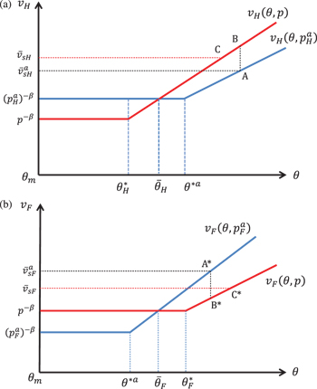
Impact of trade on the welfare distribution in each country.

According to Figure 1(a), after trade liberalization individuals with θ>θˉH experience an increase in their welfare, whereas individuals with θ<θˉH experience a decrease in their welfare. In Foreign, the welfare of all workers with θ∈[1,θˉF) increases, but the welfare of workers with θ>θˉF falls. Trade has no impact on the welfare of the individual with ability θˉj; i.e., vj(θˉj,p)=vj(θˉj,pja). Substituting the corresponding equations from [19] into vj(θˉj,p)=vj(θˉj,pja) and using p/pja=(θ∗a/θj∗)1/2 from eq. [7] yields

To determine the impact of trade on aggregate welfare, consider the aggregate welfare function given by eq. [13]. The welfare function [13] is convex, and the necessary condition for minimizing Vj yields the equilibrium condition [14]. ^[11] Thus, trade is welfare improving. ^[12] The following proposition summarizes these results.

1. raises (lowers) the welfare of all individuals with1≤θ<θˉH(1≤θ<θˉF), but it lowers (raises) the welfare of all individuals withθ>θˉH(θ>θˉF) in Home (Foreign).

2. improves the aggregate welfare in both countries.

Having determined the impact of trade on the welfare distribution, I now turn to investigate the impact of trade on inequality. Before going further, note that the welfare eq. [3] implies

for any two individuals with θ1 and θ2 in country j. That is, the welfare inequality and income inequality represent the same thing, and therefore in the subsequent discussion I will call them inequality. In investigating the impact of trade on inequality, I consider its impact on between-group and within-group inequalities. Consider first the inequality between skilled and unskilled workers, and following much of the literature on income inequality, I define between-group inequality in country j as the ratio of the average income of skilled workers (denoted by eˉsj) to the average income of unskilled workers (denoted by eˉuj). Note that eˉuj=1, since any unskilled worker’s wage equals one. The between-group inequality is then given by

The inequality between skilled and unskilled workers in autarky has the same form except θj∗ is replaced by θ∗a. Trade increases [decreases] both the aggregate income of skilled workers and their supply in Home [Foreign]. Thus, the net impact of trade on between-group income inequality in each country is ambiguous.

To get a more precise prediction, I assume that ability is (truncated) Pareto distributed: G(θ)=[1−θ−k]/[1−θM−k], with shape parameter k>1. Using a Pareto distribution makes analysis more tractable and has been widely used in trade and productivity literature (e.g., Helpman, Itskhoki, and Redding 2010). In addition, eq. [7] ensures that the corresponding human capital (and thus, firms’ productivity) levels also follow a Pareto distribution. This is consistent with several empirical studies, which have shown that firm sizes follow Pareto distribution (Axtell 2001; Helpman, Melitz, and Yeaple 2004). It is straightforward to show that

where for notational simplicity the country index j is dropped.

Note that if θM→∞, the distribution becomes standard Pareto; in this case, eˉsja/eˉuja=eˉsj/eˉuj=k/(k−1). Thus, trade has no impact on the inequality between skilled and unskilled workers in either country if ability is standard Pareto distributed. However, if θM is finite, one can show that eˉsHa/eˉuHa<eˉsH/eˉuH and eˉsFa/eˉuFa>eˉsF/eˉuF.^[13] That is, trade increases [decreases] the inequality between skilled and unskilled workers in skill-abundant Home [Foreign] as shown in Figure 1(a) [Figure 1(b)].

I now turn to analyze the impact of trade on within-group income inequality in each country. Note that there is no variation among the income of unskilled workers, because their income is always equal to one. Following much of the literature, I measure the income inequality among skilled workers by Gini coefficient. Assuming that ability is truncated Pareto distributed, the Gini coefficient for skilled workers in each country is given by (see Appendix B)

where k>1 is the shape parameter and θM is the upper bound of its support. The corresponding coefficient in autarky has the same form except θj∗ is replaced by θ∗a.

Note that under the standard Pareto distribution (i.e., θM→∞), the Gini is given by Gj=1/(2k−1); as a result, trade has no impact on the inequality among skilled workers in each country. What happens to the within-group inequality in each country after they trade when θM is finite? Figure 2 shows how the Gini coefficient changes with respect to the ability cutoff θj∗ under different shape parameters. It indicates that the impact of trade on the Gini coefficient for skilled workers in each country is ambiguous. The following proposition summarizes these results.

Figure 2

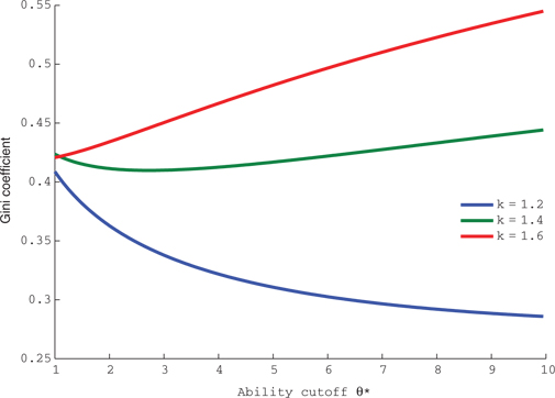
Gini coefficient with respect to ability cutoff.

1. If ability is standard Pareto distributed, trade has no impact on the between-group and within-group inequality in either country.

2. If ability is truncated Pareto distributed, trade increases [decreases] the between-group inequality in Home [Foreign]; but it has an ambiguous effect on the within-group inequality in each country.

The above results are different from the Stolper-Samuelson theorem in the standard HO model in two important ways. First, if the human capital endowment in each country had not changed after the trade liberalization, the income inequality between skilled and unskilled workers in Home would have increased by the amount predicted by the Stolper-Samuelson theorem. This effect is represented by moving from point A to B in Figure 1(a). However, in the present model, trade changes the human capital in each country both in extensive and intensive margins which in turn put a downward pressure on the inequality between these groups. In this case, the average entrepreneurial income in Home will move from point B to C in Figure 1(a). Indeed, according to Proposition 2, where ability is distributed standard Pareto, this downward pressure exactly cancels out the Stolper-Samuelson effect. ^[14] The corresponding effects in Foreign are represented by moving from A∗ to B∗ to C∗ in Figure 1(b). In sum, the impact of trade on between-group inequality in the present model is not as strong as that in the standard HO model.

Second, since in the HO model factor endowments are fixed and all skilled workers have the same level of human capital, the model is not suitable for analyzing the impact of trade on within-group inequality. In the present model, however, factor endowments are endogenously determined, and the income of skilled workers is proportional to the level of human capital they acquired. As a result, one can analyze the impact of trade on within-group inequality.

What empirical implications can one draw from the present model? The wage gap between skilled and unskilled workers has dramatically increased since the early 1980s in many developed countries and especially in the U.S. This dramatic change in the wage structure combined with increased globalization with developing countries during the same period led some economists to conclude that trade with developing countries accounts for a large share of the inequality (Wood 1998). However, the present model suggests that trade can not be a driving factor behind the growth in the skill-premium. ^[15] In addition, the skill-premium has increased in many developing countries after they opened to trade in the 1980s and 1990s (Goldberg and Pavcnik 2007). Finally, the present model predicts that the impact of trade on the wage dispersion among skilled workers is ambiguous, which suggests that trade may not be the driving factor behind the increased wage dispersion within occupations and sectors observed in many countries (Goldberg and Pavcnik 2007). ^[16]

3.3 Political-economy equilibrium

Although trade increases aggregate welfare, not all agents gain from the free trade. Is trade a viable option? To answer this question, I make two further assumptions. First, I assume that a country follows a free trade policy if the median voter prefers free trade to autarky. In other words, a country chooses to trade if the majority of its population approves it. ^[17] Second, I assume that ability follows the following Pareto distribution: G(θ)=1−θ−k, where k>1 is the shape parameter. ^[18]

Under this distribution function, the aggregate welfare function [13] then becomes,

and attains its (global) minimum at ^[19]

Using eqs [7] and [17] together with the Pareto distribution, it is straightforward to show that under free trade the ability cutoffs are given by

where θ∗a is given by eq. [22]. Note that θH∗ decreases in b, whereas θF∗ increases in it.

Since all Home workers with θ>θˉH benefit from free trade (see Figure 1.a), Home chooses to trade under majority voting if and only if G(θˉH)<0.5. Equations [20] and [23] then yield

Observe that 2β(k−1)/(2k−β)<1, and the latter inequality implies that γH<1. If γH<0, then there is no b∈R+ that satisfies the condition b−k<γH. In this case, Home chooses not to trade. Note that γH is always negative whenever β≤0.5. In addition, it increases with k. Thus, the condition γH>0 holds when β and k are sufficiently high. ^[20] In this case, Home chooses to trade if b>γH−1/k.

Foreign, on the other hand, chooses to trade under majority voting if and only if G(θˉF)>0.5. Following the same steps as in the previous case yields

G(θ¯F) > 0.5 ⇔ bk>γF≡2[2β(k−1)2k−β]2β−1.

Since 2β(k−1)/(2k−β)<1, it then follows that γF<1. Thus, the condition b>γF always holds. As a result, Foreign always chooses to trade.

The reason that Foreign always chooses to trade crucially depends on the assumption that ability follow a Pareto distribution. Although Pareto distribution is a heavy-tailed, it is skewed more towards left. Using this distributional assumption, it is easy to show that G(θ∗a)>1/2, i.e. more than half of the population in each country choose to become unskilled workers in autarky. ^[21] Since trade expands the fraction of unskilled workers in Foreign and these individuals are better off under free trade, it then follows that Foreign always chooses to trade.

The above proposition implies that an egalitarian government (in the sense that it gives equal voting rights to everyone) in Home will not choose to trade unless the share of manufacturing in total expenditure is sufficiently high and the cost of human capital acquisition is sufficiently low (compared to that in Foreign), because the majority of workers will be worse off. On the other hand, an egalitarian government in unskilled labor abundant Foreign will always choose to trade, because the majority of workers in Foreign will be better off under free trade. These results are broadly consistent with Dutt and Mitra (2005) who show that left-wing governments in capital-abundant countries adopt more protectionist trade policies than right-wing ones, and left-wing governments in labor-abundant countries adopt more pro-trade policies than right-wing ones.

3.4 Change in the cost of human capital acquisition

The analysis so far has focused on how trade liberalization affects allocation of skills across sectors and its effects on income distribution and welfare in each country. Another interesting question to address is the implication of a change in the cost parameter b in one country on the income distribution and welfare in each country when countries freely trade with each other. The following lemma characterizes the impact of this change on the ability cutoff level in each country (see Appendix C for the proof).

Without loss of generality, consider a reduction in Foreign’s cost parameter bF.^[22] According to the above lemma, such a reduction decreases the ability cutoff level θF∗ in Foreign, while increasing θH∗ in Home. Thus, the fraction of individuals who acquire human capital increases (decreases) in Foreign (Home). Furthermore, eqs [5] and [7] indicate that each worker in manufacturing in Foreign will acquire more human capital. The opposite will be observed in Home. Assuming that ability is truncated Pareto distributed, the income inequality between skilled and unskilled workers increases in Foreign and decreases in Home. As shown in Appendix C, such a reduction in bF improves Foreign welfare and reduces Home welfare. Appendix C also shows that a reduction in bH (instead of bF) improves welfare in both countries. The following proposition summarizes the results assuming that such a reduction happens in Foreign.

A reduction in bF makes human capital formation more affordable in Foreign, which induces more people to work in manufacturing, i.e. the ability cutoff necessary to work in manufacturing falls in Foreign. This will increase individual-level human capital as well as the income per capita for workers in Foreign’s manufacturing. An expansion in Foreign’s manufacturing sector lowers relative price of the manufacturing good as well. This makes human capital formation more costly for some workers in Home, and thus they prefer to work in agricultural sector. In this case, the ability cutoff θH∗ will raise in Home.

A reduction in the ability cutoff in Foreign increases each manufacturing worker’s income (see eq. [10]), which increases the aggregate income in Foreign. This, combined with a reduction in the price of manufacturing, improves the aggregate welfare in Foreign. On the other hand, a fall in relative price of the manufacturing good combined with a lower human capital reduces each manufacturing worker’s income in Home. Consequently, Home aggregate income decreases. Although reduction in the price of the manufacturing good has a positive effect on welfare, reduction in aggregate income overcomes this effect, and thus, aggregate welfare decreases in Home.

In the case of a reduction in the cost of human capital in Home (i.e., bH↓), Home welfare improves since relative price of the manufacturing good decreases and the aggregate expenditure increases. Although such a reduction decreases the aggregate expenditure in Foreign, reduction in the relative price of manufacturing dominates the latter, and thus improves welfare in Foreign as well.

References

Axtell, R. 2001. “Zipf Distribution of U.S. Firm Sizes.” Science 293:1818–20.10.1126/science.1062081Suche in Google Scholar
Bombardini, M., G. Gallipoli, and G. Pupato. 2012. “Skill Dispersion and Flows of Trade.” American Economic Review 102:2327–48.10.3386/w15097Suche in Google Scholar
Bond, E. 1986. “Entrepreneurial Ability, Income Distribution and International Trade.” Journal of International Economics 20:343–56.10.1016/0022-1996(86)90026-7Suche in Google Scholar
Bonfatti, R., and M. Ghatak. 2013. “Trade and the Allocation of Talent with Capital Market Imperfections.” Journal of International Economics 89:187–201.10.1016/j.jinteco.2012.07.005Suche in Google Scholar
Borsook, I. 1987. “Earnings, Ability and International Trade.” Journal of International Economics 22:281–95.10.1016/S0022-1996(87)80024-7Suche in Google Scholar
Bougheas, S., and R. Riezman. 2007. “Trade and the Distribution of Human Capital.” Journal of International Economics 73:421–33.10.1142/9789814390125_0020Suche in Google Scholar
Bustos, P. 2011. “The Impact of Trade Liberalization on Skill Upgrading. Evidence From Argentina,” CREI Working Paper.Suche in Google Scholar
Cartiglia, F. 1997. “Credit Constraints and Human Capital Accumulation in the Open Economy.” Journal of International Economics 43:221–36.10.1016/S0022-1996(96)01469-9Suche in Google Scholar
Chesnokova, T., and K. Krishna. 2009. “Skill Acquisition, Credit Constraints, and Trade.” International Review of Economics and Finance 18:227–38.10.3386/w12411Suche in Google Scholar
Dinopoulos, E., and P. Segerstrom. 1999. “A Schumpeterian Model of Protection and Relative Wages.” American Economic Review 89:450–72.10.1257/aer.89.3.450Suche in Google Scholar
Dinopoulos, E., and B. Unel. 2013. “Entrepreneurs, Jobs, and Trade,” LSU Working Paper.10.1016/j.euroecorev.2015.07.010Suche in Google Scholar
Dinopoulos, E., and B. Unel. 2014. “Firm Productivity, Occupational Choice, and Inequality in a Global Economy,” LSU Working Paper.Suche in Google Scholar
Dutt, P., and D. Mitra. 2005. “Political Ideology and Endogenous Trade Policy: An Empirical Investigation.” Review of Economics and Statistics 87:59–72.10.3386/w9239Suche in Google Scholar
Edmonds, E. V., N. Pavcnik, and P. Topalova. 2010. “Trade Adjustment and Human Capital Investments: Evidence From Indian Tariff Reform.” American Economic Journal: Applied Economics 2:42–75.10.3386/w12884Suche in Google Scholar
Eicher, T. S. 1999. “Trade, Development and Converging Growth Rates: Dynamic Gains From Trade Reconsidered.” Journal of International Economics 48:179–98.10.1016/S0022-1996(98)00028-2Suche in Google Scholar
Epifani, P., and G. A. Gancia. 2008. “The Skill Bias of World Trade.” Economic Journal 118:927–60.10.1111/j.1468-0297.2008.02156.xSuche in Google Scholar
Ferguson, D. G. 1978. “International Capital Mobility and Comparative Advantage: The Two-Country, Two-Factor Case.” Journal of International Economics 8:373–96.10.1016/0022-1996(78)90002-8Suche in Google Scholar
Findlay, R., and H. Kierzkowsi. 1983. “Human Capital and International Trade: A Simple General Equilibrium Model.” Journal of Political Economy 91:957–78.10.1086/261195Suche in Google Scholar
Galor, O., and D. Mountford. 2008. “Trading Population for Productivity: Theory and Evidence.” Review of Economic Studies 75:1143–79.10.1111/j.1467-937X.2008.00501.xSuche in Google Scholar
Goldberg, P. K., and N. Pavcnik. 2007. “Distributional Effects of Globalization in Developing Countries.” Journal of Economic Literature 45:39–92.10.3386/w12885Suche in Google Scholar
Grossman, G. M., and G. Maggi. 2000. “Diversity and Trade.” American Economic Review 90:1255–75.10.3386/w6741Suche in Google Scholar
Helpman, E., O. Itskhoki, and S. Redding. 2010. “Inequality and Unemployment in a Global Economy.” Econometrica 78:1239–83.10.3386/w14478Suche in Google Scholar
Helpman, E., M. J. Melitz, and S. R. Yeaple. March 2004. “Export Versus FDI with Heterogeneous Firms.” American Economic Review 94:300–16.10.1257/000282804322970814Suche in Google Scholar
Ishikawa, J. 1996. “Scale Economies in Factor Supplies, International Trade, and Migration.” Canadian Journal of Economics 29:573–94.10.2307/136251Suche in Google Scholar
Lucas, R. E. 1978. “On the Size Distribution of Business Firms.” Bell Journal of Economics 9:508–23.10.2307/3003596Suche in Google Scholar
Ma, L. 2014. “Globalization and Top Income Shares.” National University of Singapore, Working Paper.Suche in Google Scholar
Mas-Colell, A., M. D. Winston, and J. R. Green. 1995. Microeconomic Theory. New York, NY: Oxford University Press.Suche in Google Scholar
Mayer, W. 1984. “Endogenous Tariff Formation.” American Economic Review 74:970–85.Suche in Google Scholar
O’Rourke, K. H., A. S. Rahman, and A. M. Taylor. 2007. “Trade, Knowledge, and the Industrial Revolution,” NBER Working Paper No. 13057.10.3386/w13057Suche in Google Scholar
Ranjan, P. 2001. “Dynamic Evolution of Income Distribution and Credit-Constrained Human Capital Investment in Open Economies.” Journal of International Economics 55:329–58.10.1016/S0022-1996(01)00103-9Suche in Google Scholar
Unel, B. 2010. “Firm Heterogeneity, Trade, and Wage Inequality.” Journal of Economic Dynamics and Control 34:1369–79.10.1016/j.jedc.2010.03.005Suche in Google Scholar
Wood, A. 1998. “Globalisation and the Rise in the Labour Market Inequalities.” Economic Journal 108:1463–82.10.1111/1468-0297.00354Suche in Google Scholar
Yeaple, S. R. 2005. “A Simple Model of Firm Heterogeneity, International Trade, and Wages.” Journal of International Economics 65:1–20.10.1016/j.jinteco.2004.01.001Suche in Google Scholar
©2015 by De Gruyter
Artikel in diesem Heft
- Frontmatter
- Advances
- Insulation or Patronage: Political Institutions and Bureaucratic Efficiency
- Rural Property Rights, Migration, and Welfare in Developing Countries
- The Impact of Voluntary Youth Service on Future Outcomes: Evidence from Teach For America
- Contributions
- Human Capital Formation and International Trade
- Racial Discrimination in the Labor Market for Recent College Graduates: Evidence from a Field Experiment
- Life Insurance and Suicide: Asymmetric Information Revisited
- The Impact of Immigration on Native Wages and Employment
- The Effect of Pharmacies’ Right to Negotiate Discounts on the Market Share of Parallel Imported Pharmaceuticals
- Vertical or Horizontal: Endogenous Merger Waves in Vertically Related Industries
- Violence in Illicit Markets: Unintended Consequences and the Search for Paradoxical Effects of Enforcement
- Topics
- The Effect of Alcohol Consumption on Labor Market Outcomes of Young Adults: Evidence from Minimum Legal Drinking Age Laws
- Impacts of FTA Utilization on Firm Performance
- Is There a Motherhood Wage Penalty for Highly Skilled Women?
- Developers’ Incentives and Open-Source Software Licensing: GPL vs BSD
- Noise or News? Learning about the Content of Test-Based School Achievement Measures
- Entrepreneurial Risk Choice and Credit Market Equilibria
- How Responsive Are EU Coal-Burning Plants to Changes in Energy Prices?