Local Option, Alcohol and Crime
-
Stephen B. Billings


Abstract
With the end of National Prohibition in 1933, 30 states gave counties and municipalities the local option to continue alcohol restrictions. Currently, 10% of U.S. counties still maintain a ban on some or all alcohol. Since the Prohibition movement advanced on the association between alcohol use and criminal behavior, this research examines the impact of county-level alcohol restrictions on multiple types of crime across five U.S. states. Standard panel models show a positive relationship between local option policy changes to allow alcohol and crime. The novelty of this research involves comparing the impact of alcohol restrictions across crimes classified by the degree to which an offense is often committed under the influence of alcohol. Results highlight impacts across a number of crime categories with crimes commonly committed under the influence of alcohol as well as crimes involving drug use and even crimes associated with obtaining alcohol all increasing when counties allow the sale and consumption of alcohol.
Acknowledgments
This research benefited from discussions with Jennifer Troyer and Craig Depken II as well as participants at the University of North Carolina Charlotte economics seminar and the Southern Economic Association 2009 meetings.
Appendix: propensity score matching
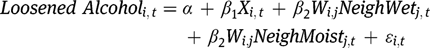
Propensity Score Matching has been applied in economics by a number of scholars33 in order to create control groups in non-experimental settings. The premise behind our propensity score matching estimator is to sample from all counties that did not enact local option between 1994 and 2006, but contain similar observable characteristics to local option counties in the year before the change in local option policy. This sampling provides a comparison group for local option counties. Since we focus on local option changes that Allowed Alcohol as well as Loosened Alcohol restrictions, we implement PSM separately for these forms of local option. We begin by estimating eq. [3] for  and eq. [4] for
  . We define
  and
and  slightly differently in implementing PSM. Here, they are given a one only for local option counties in the year of the local option election and zero otherwise. Given the observed spatial dependence in alcohol polices, we include indicators for neighboring county’s alcohol status by
  and
and  .34 Propensity score estimation results are available in Table 7 and highlight that per capita income, percent high school graduates, percent college graduates and percent baptists have a positive influence while percent democratic votes and total offenses had a negative influence on local option changes to allow alcohol. Percent democratic votes, percent high school graduates, percent college degrees, population density, total offenses and portion of neighboring counties that are Moist had a positive influence, while percent of the population over 65 had a negative influence on local option changes that loosened alcohol restrictions. Predicted values for
  and
and  represent our propensity score.

PSM requires that all independent variables are similar within a given strata of estimated propensity scores (balancing assumption) as well as that estimated propensity scores for both local option and non-local option counties occur across similar values (common data support). A formal test of the balancing assumption is implemented for the all independent variables included in the propensity score estimation as outlined in Dehejia and Wahba (2002). This test found that propensity scores and covariates were insignificantly different between treatment and comparison groups within a given strata at the 5% level. To satisfy the common data support assumption, we only considered estimated propensity scores for observations that occur in the range of possible values for all counties.35
This research adopts two different matching algorithms in order to test the robustness of results. We implemented matching separately for Allowed Alcohol and Loosened Alcohol local option counties and only considered dry counties and moist counties as possible matches respectively. First, we implement a nearest neighbor with replacement algorithm, which matches each county that implemented local option in year t with a potential comparison county in year t that contains the nearest valued propensity score. This matching provides a single comparison county to match with each treatment county in the same year. The second matching algorithm selects the five nearest neighbors that are within a caliper difference from the treatment county’s propensity score. We set the caliper value at 0.01 and limit matches to be based on the year of a given county’s local option change. We impose a common support for all matching algorithms, which removes the possibility of matching treatment observations with propensity scores outside the range of propensity scores for treatment counties.36
PSM first stage regressions
Dep Var  | Allowed Alcohol | Loosened Alcohol |
| Per capita income | 0.021** | 0.019 |
| (0.009) | (0.023) | |
| Unemploy rate | 0.036 | –0.349 |
| (3.231) | (4.570) | |
| Percent black pop | 0.510 | –0.974 |
| (0.599) | (0.792) | |
| Percent Hispanic pop | 0.176 | –2.107 |
| (0.747) | (4.315) | |
| Percent democratic votes | –1.800*** | 2.747*** |
| (0.601) | (1.016) | |
| Median age | –0.048 | 0.091 |
| (0.037) | (0.080) | |
| Percent pop over 65 | 4.449 | –13.751** |
| (3.140) | (6.885) | |
| Percent pop under 18 | –0.989 | 5.780 |
| (2.368) | (5.860) | |
| Percent high sch grads | 2.866** | 8.712*** |
| (1.404) | (2.683) | |
| Percent college degree | 2.281** | 3.885* |
| (0.996) | (2.098) | |
| Percent Baptists | 1.426*** | 0.799 |
| (0.405) | (0.588) | |
| Percent Catholics | 0.232 | –4.144 |
| (0.647) | (2.943) | |
| Pop density | 0.001 | 0.003** |
| (0.001) | (0.002) | |
| Pop growth | 1.189 | 1.512 |
| (1.452) | (2.607) | |
| Total offenses | –0.014*** | 0.009** |
| (0.005) | (0.005) | |
| Police expend | –0.010 | –0.031 |
| (0.014) | (0.021) | |
| Neigh wet | –0.066 | 0.514 |
| (0.336) | (0.624) | |
| Neigh moist | –0.310 | 1.125* |
| (0.319) | (0.584) | |
| Observations | 8,268 | 8,268 |
| Psuedo R2 | 0.13 | 0.23 |
References
Baughman, R., M.Conlin, S.Dickert-Conlin, and J.Pepper. 2001. “Slippery When Wet: The Effects of Local Alcohol Access Laws on Highway Safety.” Journal of Health Economics20(6):1089–96.10.1016/S0167-6296(01)00103-5Suche in Google Scholar
Biderman, C., J. M.DeMello, and A.Schneider. 2010. “Dry Laws and Homicides: Evidence from the So Paulo Metropolitan Area.” The Economic Journal120(543):157–82.10.1111/j.1468-0297.2009.02299.xSuche in Google Scholar
Brown, R., R.Jewell, and J.Richer. 1996. “Endogenous Alcohol Prohibition and Drunk Driving.” Southern Economic Journal62(4):1043–53.10.2307/1060947Suche in Google Scholar
Brueckner, J. 1998. “Testing for Strategic Interaction among Local Governments: The Case of Growth Controls.” Journal of Urban Economics44(3):438–67.10.1006/juec.1997.2078Suche in Google Scholar
Brueckner, J., and L.Saavedra. 2001. “Do Local Governments Engage in Strategic Property-Tax Competition?” National Tax Journal54(2):203–29.10.17310/ntj.2001.2.02Suche in Google Scholar
Carpenter, C. 2007. “Heavy Alcohol Use and Crime: Evidence from Underage Drunk-Driving Laws.” Journal of Law and Economics50(3):539–57.10.1086/519809Suche in Google Scholar
Carpenter, C., and C.Dobkin. 2009. “The Effects of Alcohol Access on Consumption and Mortality: Regression Discontinuity Evidence From the Minimum Drinking Age.” American Economic Journal – Applied Economics1(1):164–82.10.1257/app.1.1.164Suche in Google Scholar
Chaloupka, F., H.Saffer, and M.Grossman. 2002. “The Effects of Price on Alcohol Consumption and Alcohol-Related Problems.” Alcohol Research and Health26(1):22–34.Suche in Google Scholar
Conlin, M., S.Dickert-Conlin, and J.Pepper. 2005. “The Effect of Alcohol Prohibition on Illicit-Drug-Related Crimes.” Journal of Law and Economics48(1):215–34.10.1086/428017Suche in Google Scholar
Cook, P. 2007. Paying the Tab. Princeton, NJ: Princeton University Press.Suche in Google Scholar
Cook, P. J., and M. J.Moore. 2002. “The Economics of Alcohol Abuse and Alcohol-Control Policies.” Health Affairs21(2):120–33.10.1377/hlthaff.21.2.120Suche in Google Scholar
Dehejia, R., and S.Wahba. 2002. “Propensity Score-Matching Methods for Nonexperimental Causal Studies.” Review of Economics and Statistics84(1):151–61.10.1162/003465302317331982Suche in Google Scholar
Distilled Spirits Council.1940–1970. “Annual Statistical Review of the Distilled Spirits Industry,” Research and Statistical Division.Suche in Google Scholar
Dull, R., and D.Giacopassi. 1988. “Dry, Damp, and Wet – Correlates and Presumed Consequences of Local Alcohol Ordinances.” American Journal of Drug and Alcohol Abuse14(4):499–514.10.3109/00952998809001567Suche in Google Scholar
Eisenberg, D. 2003. “Evaluating the Effectiveness of Policies Related to Drunk Driving.” Journal of Policy Analysis and Management22(2):249–74.10.1002/pam.10116Suche in Google Scholar
Graham, K., S.Bernards, D. W.Osgood, and S.Wells. 2006. “Bad Nights or Bad Bars? Multi-Level Analysis of Environmental Predictors of Aggression in Late-Night Large-Capacity Bars and Clubs.” Addiction101(11):1569–80.10.1111/j.1360-0443.2006.01608.xSuche in Google Scholar
Gyimah-Brempong, K. 2001. “Alcohol Availability and Crime: Evidence from Census Tract Data.” Southern Economic Journal68(1):2–21.Suche in Google Scholar
Heaton, P. 2012. “Sunday Liquor Laws and Crime.” Journal of Public Economics96(1–2):42–52.10.1016/j.jpubeco.2011.08.002Suche in Google Scholar
Homel, R., S.Tomsen, and J.Thommeny. 1992. “Public Drinking and Violence – Not Just an Alcohol Problem.” Journal of Drug Issues22(3):679–97.10.1177/002204269202200315Suche in Google Scholar
Lang, A., and P.Sibrel. 1989. “Psychological Perspectives on Alcohol-Consumption and Interpersonal Aggression – The Potential Role of Individual-Differences in Alcohol-Related Criminal Violence.” Criminal Justice and Behavior16(3):299–324.10.1177/0093854889016003004Suche in Google Scholar
List, J., D.Millimet, P.Fredriksson, and W.McHone. 2003. “Effects of Environmental Regulations on Manufacturing Plant Births: Evidence From a Propensity Score Matching Estimator.” Review of Economics and Statistics85(4):944–52.10.1162/003465303772815844Suche in Google Scholar
Markowitz, S. 2005. “Alcohol, Drugs and Violent Crime.” International Review of Law and Economics25(1):20–44.10.1016/j.irle.2005.05.003Suche in Google Scholar
Mast, B., B.Benson, and D.Rasmussen. 1999. “Beer Taxation and Alcohol-Related Traffic Fatalities.” Southern Economic Journal66:214–49.Suche in Google Scholar
Miron, J., and E.Tetelbaum. 2009. “Does the Minimum Legal Drinking Age Save Lives?” Economic Inquiry47(2):317–36.10.1111/j.1465-7295.2008.00179.xSuche in Google Scholar
Mocan, N., and E.Tekin. 2006. “Catholic Schools and Bad Behavior: A Propensity Score Matching Analysis.” Contributions to Economic Analysis and Policy5(1):1–34.Suche in Google Scholar
O’Keefe, S. 2004. “Job Creation in California’s Enterprise Zones: A Comparison Using a Propensity Score Matching Model.” Journal of Urban Economics55(1):131–50.10.1016/j.jue.2003.08.002Suche in Google Scholar
Powers, E., and J.Wilson. 2004. “Access Denied: The Relationship Between Alcohol Prohibition and Driving Under the Influence.” Sociological Inquiry74(3):318–37.10.1111/j.1475-682X.2004.00094.xSuche in Google Scholar
Smith, J., and P.Todd. 2005. “Does Matching Overcome LaLonde’s Critique of Nonexperimental Estimators?” Journal of Econometrics125(1–2):305–53.10.1016/j.jeconom.2004.04.011Suche in Google Scholar
Spunt, B., P.Goldstein, H.Brownstein, M.Fendrich, and S.Langley. 1994. “Alcohol and Homicide – Interviews with Prison-Inmates.” Journal of Drug Issues24(1–2):143–63.10.1177/002204269402400108Suche in Google Scholar
Strumpf, K., and F.Oberholzer-Gee. 2002. “Endogenous Policy Decentralization: Testing the Central Tenet of Economic Federalism.” Journal of Political Economy110(1):1–36.10.1086/324393Suche in Google Scholar
Toomey, T., and A.Wagenaar. 2002. “Environmental Policies to Reduce College Drinking: Options and Research Findings.” Journal of Studies on Alcohol14:193–205.10.15288/jsas.2002.s14.193Suche in Google Scholar
U.S. Department of Justice.2002. “Bureau of Justice Statistics.” Survey of Inmates in Local Jails.Suche in Google Scholar
U.S. Department of Justice.2004. “Bureau of Justice Statistics.” Survey of Inmates in State and Federal Correctional Facilities.Suche in Google Scholar
Winn, R., and D.Giacopassi. 1993. “Effects of County-Level Alcohol Prohibition on Motor-Vehicle Accidents.” Social Science Quarterly74(4):783–92.Suche in Google Scholar
Young, D., and A.Bielinska-Kwapisz. 2006. “Alcohol Prices, Consumption, and Traffic Fatalities.” Southern Economic Journal72:690–703.Suche in Google Scholar
Young, D., and T.Likens. 2000. “Alcohol Regulation and Auto Fatalities.” International Review of Law and Economics20:107–26.10.1016/S0144-8188(00)00023-5Suche in Google Scholar
- 1
Subcounty restrictions include any county where either just the municipality or unincorporated county restrict alcohol sales and consumption. Type of alcohol restrictions indicate prohibition on a specific type of alcohol such as beer, wine or liquor.
- 2
See literature reviews by Cook (2007) and Moore (2002) and Chaloupka, Saffer, and Grossman (2002).
- 3
For example, see Carpenter (2007) for an analysis of Zero Tolerance (ZT) drunk driving laws, Markowitz (2005) for beer taxes, Eisenberg (2003) for Blood Alcohol Content (BAC) thresholds for driving under the influence (DUI) and Carpenter and Dobkin (2009) and Miron and Tetelbaum (2009) for a study of Minimum Legal Drinking Age (MLDA).
- 4
- 5
- 6
- 7
One exception is Conlin, Dickert-Conlin, and Pepper (2005), who find a negative relationship between local option changes to wet counties in Texas and drug arrests.
- 8
Specifically, we include the Survey of Inmates in Local Jails (U.S. Department of Justice 2002) and Survey of Inmates in State and Federal Correctional Facilities (U.S. Department of Justice 2004).
- 9
Arrest data represents a departure from the more commonly used UCR annual data on offenses, which is restricted to only Type I crimes (murder, rape, aggravated assault, arson, larceny, automobile theft and burglary). The limited number of Type I crime categories is problematic in understanding the effects of alcohol policies because the crimes most commonly associated with alcohol usage are absent from the offense data. There is no offense data on DUIs, public drunkenness or even simple assault.
- 10
The most widely known temperance organization was the Anti-Saloon League.
- 11
Alabama, Arkansas, Florida, Georgia, Kansas, Kentucky, Mississippi, North Carolina, Tennessee, Texas, Virginia.
- 12
We base this initial assessment of local option states on Strumpf and Oberholzer-Gee (2002), state statutes and Distilled Spirits Council (1940–1970).
- 13
This latter task is not an easy one and prevented the inclusion of Mississippi due to the role of legislative action in changing or exempting alcohol control policies at jurisdiction or even sub-jurisdictional levels. Additionally, Kansas could not be included due to missing crime data before 2000.
- 14
Ideally, we could explicitly test the effects of specific alcohol restrictions within the moist county classification. Unfortunately, the limited number of counties with local option changes for each specific moist county alcohol restriction would limit identification to only a few counties.
- 15
For example, moist counties in Alabama, North Carolina, Kentucky and Texas contained wet cities within dry counties; Tennessee moist counties do not allow liquor sales but do allow the sale of beer and wine. Moist counties in Kentucky only allow vineyards, golf courses, or restaurants with at least 70% of their sales from food to sell alcohol. North Carolina and Texas moist counties prohibit certain types of alcohol (beer, wine and/or spirits). Texas moist counties sometimes restrict on-premises liquor sales.
- 16
By years, there were 16 local option changes between 1994 and 2000; 12 between 2001 and 2002; 9 in 2003; 15 in 2004 and 8 in 2005.
- 17
Further disaggregation from dry to moist or dry to wet did not change overall conclusions and estimates for the limited number of dry to wet local option changes were inconsistent across models and contained large standard errors.
- 18
Only one county changed from wet or moist to dry. Knott county, Kentucky switched from wet to dry in 2000.
- 19
For non-annual data, annual data is generated from a linear interpolation of existing data points.
- 20
- 21
As a robustness check, we later show that our main results are similar when using total offenses per capita.
- 22
The mean number of total arrests in our sample is 52.4 per 1,000 people, while the mean number of total offenses is only 24.8 per 1,000 people.
- 23
We find only 60 out of our total of 8,268 observations with total arrests equal to zero using arrest data and 869 using offense data.
- 24
See Appendix for the details of our application of PSM.
- 25
Results incorporating an inverse distance weight matrix
 provided similar results and we include neighbors across state borders.
 - 26
We include counties in bordering states in the computation of NonDryNeighs with states not included in our dataset being considered non-dry.
- 27
In our case, caliper-based PSM provided fewer total counties included in regression analysis, but we weight observations by the frequency they are selected as a matched control county.
- 28
- 29
We exclude approximately 1/3 of survey respondents because they did not respond to the alcohol usage question. We found excluded surveys to be similar across other dimensions of survey questions.
- 30
The positive impact on drug arrests differs from the finding of Conlin, Dickert-Conlin, and Pepper (2005), but this may be a result of our inclusion of four additional states, a different data source for arrests, separate variables for local option changes from dry or from moist counties, as well as neighboring county alcohol status.
- 31
Ideally, we could measure alcohol consumption in dry counties, but given their illegality this is not possible.
- 32
These behavioral changes under the influence of alcohol are well discussed in the literature (Spunt et al. (1994) and Lang and Sibrel (1989)) as the pharmacophysiological effect of alcohol usage on criminal behavior.
- 33
- 34
 if neighbor j is a wet county in time t and
  if neighbor j is a moist county in time t.
 - 35
Results of these tests as well as histograms of propensity scores are available upon request.
- 36
The common support imposition only removed three local option counties.
©2014 by Walter de Gruyter Berlin / Boston
Artikel in diesem Heft
- Frontmatter
- Advances
- Preferential Admission and MBA Outcomes: Mismatch Effects by Race and Gender
- Quantity Uncertainty and Demand: The Case of Water Smart Reader Ownership
- Contributions
- Employment Effects of the 2009 Minimum Wage Increase: New Evidence from State-Based Comparisons of Workers by Skill Level
- Introducing Carbon Taxes in Russia: The Relevance of Tax-Interaction Effects
- Estimating Parents’ Valuations of Class Size Reductions Using Attrition in the Tennessee STAR Experiment
- Local Option, Alcohol and Crime
- To Work or Not to Work? The Effect of Childcare Subsidies on the Labour Supply of Parents
- Understanding Ransom Kidnappings and Their Duration
- Screening Stringency in the Disability Insurance Program
- Sticks and Carrots in Procurement: An Experimental Exploration
- Peer Effects and Policy: The Relationship between Classroom Gender Composition and Student Achievement in Early Elementary School
- Topics
- Competition and Innovation in Product Quality: Theory and Evidence from Eastern Europe and Central Asia
- Trading the Television for a Textbook?: High School Exit Exams and Student Behavior
- The Effect of Parental Migration on the Educational Attainment of Their Left-Behind Children in Rural China
- Do Parents’ Social Skills Influence Their Children’s Sociability?
- The Role of Infrastructure in Mitigating Poverty Dynamics: The Case of an Irrigation Project in Sri Lanka
- Congestion of Academic Journals Under Papers’ Imperfect Selection
- Endogenous Merger with Learning
- Do Low-Skilled Migrants Contribute More to Home Country Income? Evidence from South Asia
- The Minimum Wage and Crime