BatchDeconvolution: a Fiji plugin for increasing deconvolution workflow
-
Zbigniew Baster

 und
Zenon Rajfur
und
Zenon Rajfur

Abstract
Deconvolution microscopy is a very useful, software-based technique allowing to deblur microscopy images and increase both lateral and axial resolutions. It can be used along with many of fluorescence microscopy imaging techniques. By increasing axial resolution, it also enables three-dimensional imaging using a basic wide-field fluorescence microscope. Unfortunately, commercially available deconvolution software is expensive, while freely available programs have limited capabilities of a batch file processing. In this work we present BatchDeconvolution, a Fiji plugin that bridges two programs that we used subsequently in an image deconvolution pipeline: PSF Generator and DeconvolutionLab2, both from Biomedical Imaging Group, EPFL. Our software provides a simple way to perform a batch processing of multiple microscopy files with minimal working time required from the user.
Introduction
Fluorescence microscopy is one of the most commonly used techniques in life sciences. The use of fluorescent probes allowed to tag specific proteins and structures within live or fixed cells and image them with high contrast and resolution [1]. Using a relatively low-cost fluorescence microscope, it is possible to achieve the lateral resolution as low as 200 nm [2]. Unfortunately, it is much harder to reach high resolution along the Z optical axis, therefore three-dimensional (3D) imaging is much more challenging [2]. There is a number of microscopy techniques allowing 3D imaging, such as confocal microscopy, 3D structured illumination microscopy, 3D stochastic optical reconstruction microscopy/photoactivated localization microscopy or light sheet microscopy, but most of them require additional, usually expensive, modules, which have to be mounted on a microscope [3].
Deconvolution microscopy is one of a few techniques that do not require any additional hardware. Based on a computational image reconstruction, it can improve both lateral and axial resolutions, allowing 3D imaging without any additional equipment cost [4]. Nevertheless, one of the main drawbacks of this technique is the requirement of vast amount of calculations, what significantly extends image preparation time [5]. Secondly, in comparison to other techniques, the intensity-based quantitative analysis on deconvolved images is much more challenging due to nonlinear operations required for image reconstruction [6].
An image of a single bright point is visible as a characteristic diffraction-based pattern called point spread function (PSF) (Figure 1A) which is specific for every optical set-up [4]. It is shaped due to physical limitation of light, physical limitations of imaging environment, and also defects and imperfections present in the imaging system. An image of a physical object (e.g. a cytoskeleton or an organelle) is a superposition of many single bright points convolved with the PSF [4]:
image=object∗PSF.
![Figure 1: Panel A shows exemplary cross-section images of a point spread function (PSF) generated with PSF Generator using Gibson-Lanni algorithm [22]. The green lines show the orientations of the cross-sections. Image saturation level was set to 0.01 (high saturation). PSF generation parameters: NA = 1.4, ni = 1.518, ns=1.33, λ = 561 nm, ti = 170 µm, zp = 2,000 nm. Based on a study by Kirshner et al. [8]. Panel B shows an example of a deconvolved image of immunofluorescence staining of proteasomes (PSMA2 marker) in MDA-MB-231 cells (full description in a study by Baster et al. [20]). The image was collected as a z-stack of 21 slices, one of the representative intermediate slices is presented. The brightness and contrast parameter was chosen to cover 50–99% of the pixel brightness histogram, separately in the predeconvolution and postdeconvolution images. Mpl-inferno LUT was used. Panel C shows the microscopy image acquisition-analysis pipeline. After acquisition, depending on a type of microscopy and analysis required, image may be enhanced (e.g. reconstructed or deconvolved) and then subjected to image analysis, or analysed without any additional intermediate steps. The final step is the data extraction, statistical analysis (if applicable), and preparation of a figure for presentation. Each of the steps can be automated to some extent.](/document/doi/10.1515/bams-2020-0027/asset/graphic/j_bams-2020-0027_fig_001.jpg)
Panel A shows exemplary cross-section images of a point spread function (PSF) generated with PSF Generator using Gibson-Lanni algorithm [22]. The green lines show the orientations of the cross-sections. Image saturation level was set to 0.01 (high saturation). PSF generation parameters: NA = 1.4, ni = 1.518, ns=1.33, λ = 561 nm, ti = 170 µm, zp = 2,000 nm. Based on a study by Kirshner et al. [8]. Panel B shows an example of a deconvolved image of immunofluorescence staining of proteasomes (PSMA2 marker) in MDA-MB-231 cells (full description in a study by Baster et al. [20]). The image was collected as a z-stack of 21 slices, one of the representative intermediate slices is presented. The brightness and contrast parameter was chosen to cover 50–99% of the pixel brightness histogram, separately in the predeconvolution and postdeconvolution images. Mpl-inferno LUT was used. Panel C shows the microscopy image acquisition-analysis pipeline. After acquisition, depending on a type of microscopy and analysis required, image may be enhanced (e.g. reconstructed or deconvolved) and then subjected to image analysis, or analysed without any additional intermediate steps. The final step is the data extraction, statistical analysis (if applicable), and preparation of a figure for presentation. Each of the steps can be automated to some extent.
The goal of deconvolution algorithms is to reverse this process. There are two ways of obtaining a PSF. First is to measure the actual PSF on a microscope using, for example, nanometre-sized fluorescent beads [7]. This solution accounts for many of the deviations in the experimental set-up (such as flaws in the optical pathway), but the resolution of the PSF is limited by a signal-to-noise ratio, and it requires a demanding experimental procedure [7], [8]. The second approach is to calculate a theoretical PSF using one of the models approximating the optical set-up [8]. It is not restricted by the resolution limitations and it is noise free but usually cannot imitate defects of the optical set-up, as well as the experimental one [5]. Moreover, depending on the complexity of the model and its accuracy, the calculations can be highly time consuming. Whether it is better to use an experimental or a theoretical PSF it needs to be evaluated on a case-by-case basis [5].
There are several deconvolution algorithms that depend on different approaches and mathematical models and have different strengths and limitations [4], [9]. Most of them (if not all) carry out calculations in Fourier space to simplify operations [10]. Deconvolution can be applied to regular wide-field microscopy and also to standard 3D techniques, such as confocal microscopy, in order to further increase contrast and resolution (Figure 1B) [11], [12]. Beside reducing out of focus light, deconvolution can also be used for deblurring single-slice images.
There are several commercially available deconvolution software such as Huygens (Scientific Volume Imaging) or AutoQuant X3 (Media Cybernetics) allowing batch processing of many images. Their main drawback is their high cost. There are several free, usually open-source, alternatives, such as DeconvolutionLab and DeconvolutionLab2 (Biomedical Imaging Group, EPFL) [9], Iterative Deconvolve 3D (OptiNav) [13], or Parallel Iterative Deconvolution (Piotr Wendykier) [14]. They are in general less user-friendly than commercial ones and they have limited batch processing capabilities, especially in cases requiring more than one PSF such as multichannel images.
The microscopy image acquisition-analysis pipeline can be separated into several stages, that, to some extent, might be automated (Figure 1C). One of the facts advocating for automatization, is that it increases data processing reproducibility. Furthermore, it also serves as an additional pair (or rather many pairs) of hands allowing one to address one’s attention to other matters, after starting calculations.
In this work, we present BatchDeconvolution a bridging Fiji plugin, allowing a batch processing of multiple optical microscopy images. The software employs currently available programs and plugins for PSF generation and deconvolution, binding them together, providing a user-friendly deconvolution platform of multiposition, time-lapse, multichannel, z-stack raw (“straight from a microscope”) image files.
Material and methods
PSF Generator [8] v. 18.12.2017 was downloaded from http://bigwww.epfl.ch/algorithms/psfgenerator/, and its source code was obtained from https://github.com/Biomedical-Imaging-Group/PSFGenerator. DeconvolutionLab2 [9], version 2.1.2 was downloaded from http://bigwww.epfl.ch/deconvolution/deconvolutionlab2/, and its source code was obtained from https://github.com/Biomedical-Imaging-Group/DeconvolutionLab2. FFTW2 dynamic libraries for DeconvolutionLab2 were downloaded from http://bigwww.epfl.ch/deconvolution/deconvolutionlab2/.
The software was developed using Java 1.8 (Oracle) in NetBeans IDE 8.2 environment (Oracle). It was tested using Fiji [15] and ImageJ [16].
Results and discussion
During our research in the field of cell migration and mechanotransduction, we have found that using elastic polyacrylamide gels [17] to mimic tissue stiffness causes blurring and distortion of microscopy images. It is a result of a more complex optical set-up than in a case of cells plated directly on a glass or a plastic substrate. This phenomenon impedes the analysis of obtained images. By applying image deconvolution, we were able to improve quality of these images. Unfortunately, at that point none of the freely available software allowed us a batch files processing to the satisfactory extent. Furthermore, because we were often collecting confocal images of different image and voxel sizes, we needed to calculate a PSF matching every of our images. To address this problem, we checked several ImageJ/Fiji plugins allowing to calculate a theoretical PSF and to deconvolve images. We determined that the most suitable programs to use in a batch processing would be PSF Generator [8] and DeconvolutionLab (and later DeconvolutionLab2, that was applied in the final version of our software) [9] from Biomedical Imaging Group, EPFL. First, both are accessible from a command line (Fiji or system), what is essential for scripting. Secondly, they both offer a vast range of algorithms and a user-friendly environment. Although, DeconvolutionLab and DeconvolutionLab2 provide an option of batch image processing, their application is limited. Thus, we decided to develop a separate software that would meet our requirements (see Table 1 for comparison of batch processing algorithms properties between programs).
The comparison of batch processing properties of different software.
| Property | DeconvolutionLab | DeconvolutionLab2 | BatchDeconvolution |
|---|---|---|---|
| Batch image processing | Yes (processing of the whole directory) | Yes (each file has to be scripted separately) | Yes (processing of the whole directory) |
| Multichannel images processing | No | No | Yes (all files have to have the same channel structure) |
| Time-lapse images processing | No | No | Yes |
| Multiposition files processing | No | No | Limited (all positions have to have the same acquisition parameters i.e. number of frames, slices, channel and resolution) |
| PSF generation | No | Limited (basic algorithms) | Yes (automatic matching parameters with the image) |
| Image preparation (raw image processing) | Channel, time point and multiposition splitting required | Channel, time point and multiposition splitting required | Not required |
PSF, point spread function.
We implemented both programs into our new bridging Fiji plugin we named BatchDeconvolution. The graphical user interface was created to mirror most of the options from the base programs (Supplementary Figure 1). We implemented also BioFormats repository [18] to enable read-out of most of the popular image formats including their metadata. The access to metadata allowed us to process images of a different voxel and image sizes and number of time points. Therefore, the only common parameter between image files has to be their channel structure which is defined ununiformly between file formats. Because calculations create a high amount of intermediate data (from 2 to 9 times of the size of the original data), we made our plugin to process files in a sequential manner with several check points allowing to delete expendable files (Figure 2, Supplementary Data: Pseudocode). We also implemented option for providing an external PSF (e.g. experimental).
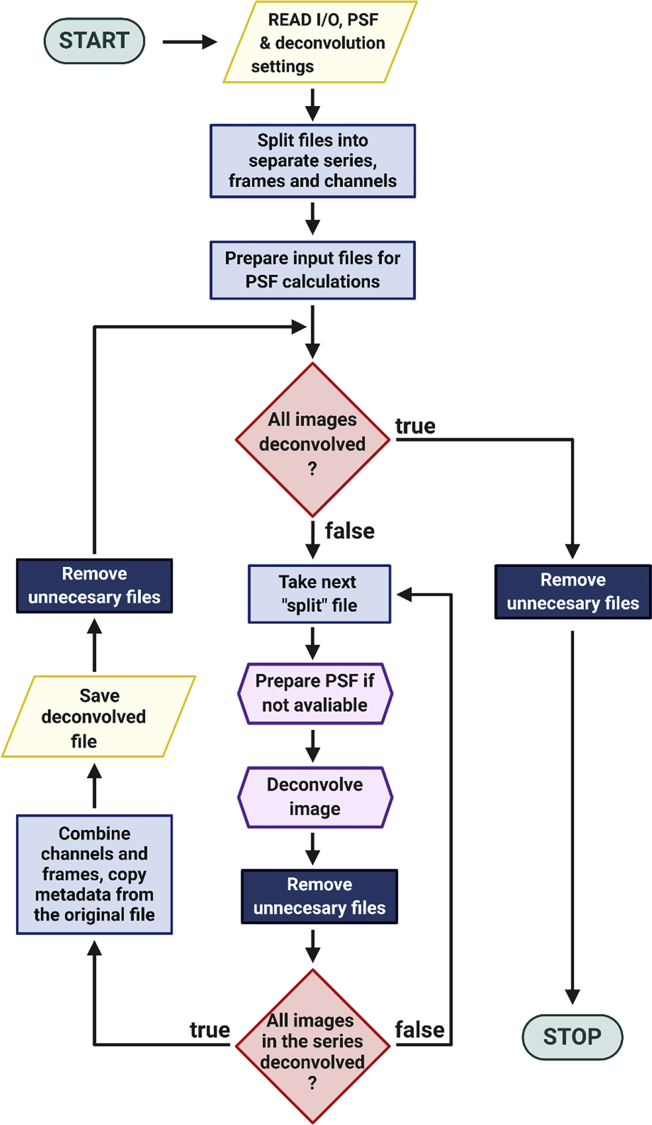
A simplified flowchart of the BatchDeconvolution’s algorithm.
Algorithm testing
We checked our software at all crucial stages of the development for generating results identical to the ones generated by the stand-alone base software (PSF Generator and DeconvolutionLab2). For format compatibility tests, we used all the images available from The Open Microscopy Environment sample images repository [19]. We run the tests on Personal Computers with at least 16 GB of RAM. All the files that met the software requirements (especially: the requirement of an image to have a defined scale; and in case of a multiposition file, the requirement all of images in the file to have the same structure) passed the test. Due to the implementation of BioFormats library, we expect that our program will read all the formats covered by the library.
The software has been routinely used (one bachelor thesis, one published article [20], two manuscripts in review, two manuscripts in preparation) on several different Personal Computers, at different stages of the program’s development. Images, that we used, were collected using Nikon wide-field fluorescence microscope or Nikon A1 confocal microscope with NIS Elements Software, Zeiss LSM 710 confocal microscope with ZEN Black software, or Zeiss wide-field fluorescence microscope with ZEN Blue software (.tif, .nd2 and .czi file formats). During our work, we found that only the amount of RAM is crucial for the proper execution of calculations. We were using Personal Computers with the memory of 4–32 GB. In a small number of cases of processing large images on low-memory computers, the software was unable to finalize calculations. Running the software on a higher-RAM computer usually solved the problem. Furthermore, when we had tried to run the stand-alone base software with the same files and parameters, we got the same errors. Thus, we believe that our bridging algorithm has no or a marginal influence on the calculations performance. Other computer components affected calculations only in regard to computing time.
Conclusions
In our work, we bridged PSF Generator and DeconvolutionLab2 programs with a Fiji plugin, and we named it BatchDeconvolution. We found our solution very useful for processing and analysing large amount of microscopy images. BatchDeconvolution provides a user-friendly, intuitive interface, allowing to process a large number of images without a requirement of any additional Fiji scripting. Applying BioFormats repository allows the software to access metadata of many file formats, that simplifies preparation of program input files and parameters.
Footnotes
Citation
We would like to emphasize that while citing our software, PSF Generator [8] and DeconvolutionLab2 [9] should be cited as well.
Access
The source code and the build version of our software are available to download from https://github.com/Mechanobiology-Lab/BatchDeconvolution.
Troubleshooting
While testing, we found that repetitive calling DeconvolutionLab2 from Fiji command line causes memory build-up within the system. We overcome that by calling DeconvolutionLab2 externally from the system command line. The drawback of that solution is that Fast Fourier Transform library JTransforms [21] that was called by DeconvolutionLab2 through Fiji, is no longer available.
BatchDeconvolution was designed and tested with a fresh installation of Fiji. It is incompatible with a clean version of ImageJ.
Funding source: Polish National Science Centre PRELUDIUM
Award Identifier / Grant number: 2018/31/N/NZ3/02031
Funding source: Polish National Science Centre ETIUDA
Award Identifier / Grant number: 2019/32/T/NZ3/00444
Acknowldgements
The authors would like to thank Olga Adamczyk (Institute of Physics, Jagiellonian University) for providing images for testing the software and Miranda Lin (Markey Cancer Center, University of Kentucky) for insightful comments on the project.
Research funding: This work was supported by the Polish National Science Centre PRELUDIUM grant no. 2018/31/N/NZ3/02031 (to ZB), and the Polish National Science Centre ETIUDA scholarship no. 2019/32/T/NZ3/00444 (to ZB).
Author contributions: Z.B. designed and wrote the software, performed tests, and wrote the manuscript; Z.R. supervised software testing and contributed to the manuscript discussion and writing. All the authors have accepted responsibility for the entire content of this submitted manuscript and approved submission.
Competing interests: The funding organization(s) played no role in the study design; in the collection, analysis, and interpretation of data; in the writing of the report; or in the decision to submit the report for publication.
Ethical approval: The conducted research is not related to either human or animal use.
References
1. Drummen, G. Fluorescent probes and fluorescence (microscopy) techniques — illuminating biological and biomedical research. Molecules 2012;17:14067–90. https://doi.org/10.3390/molecules171214067.Suche in Google Scholar
2. Combs, CA, Shroff, H. Fluorescence microscopy: a concise guide to current imaging methods. Curr Protoc Neurosci 2017;79. https://doi.org/10.1002/cpns.29.Suche in Google Scholar
3. Fischer, RS, Wu, Y, Kanchanawong, P, Shroff, H, Waterman, CM. Microscopy in 3D: a biologist’s toolbox. Trends Cell Biol 2011;21:682–91. https://doi.org/10.1016/j.tcb.2011.09.008.Suche in Google Scholar
4. Sibarita, JB. Deconvolution microscopy. Adv Biochem Eng Biotechnol 2005;95:201–43. https://doi.org/10.1007/b102215.Suche in Google Scholar
5. McNally, JG, Karpova, T, Cooper, J, Conchello, JA. Three-dimensional imaging by deconvolution microscopy. Methods 1999;19:373–85. https://doi.org/10.1006/meth.1999.0873.Suche in Google Scholar
6. Lee, JS, Wee, TLE, Brown, CM. Calibration of wide-field deconvolution microscopy for quantitative fluorescence imaging. J Biomol Tech 2014;25:31–40. https://doi.org/10.7171/jbt.14-2501-002.Suche in Google Scholar
7. Cole, RW, Jinadasa, T, Brown, CM. Measuring and interpreting point spread functions to determine confocal microscope resolution and ensure quality control. Nat Protoc 2011;6:1929–41. https://doi.org/10.1038/nprot.2011.407.Suche in Google Scholar
8. Kirshner, H, Aguet, F, Sage, D, Unser, M. 3-D PSF fitting for fluorescence microscopy: implementation and localization application. J Microsc 2013;249:13–25. https://doi.org/10.1111/j.1365-2818.2012.03675.x.Suche in Google Scholar
9. Sage, D, Donati, L, Soulez, F, Fortun, D, Schmit, G, Seitz, A, et al. DeconvolutionLab2: an open-source software for deconvolution microscopy. Methods 2017;115:28–41. https://doi.org/10.1016/j.ymeth.2016.12.015.Suche in Google Scholar
10. Swedlow, JR. Quantitative fluorescence microscopy and image deconvolution. In: Methods in cell biology. Cambridge, MA: Academic Press; 2013:407–26 pp.10.1016/B978-0-12-407761-4.00017-8Suche in Google Scholar PubMed
11. Boutet de Monvel, J, Le Calvez, S, Ulfendahl, M. Image restoration for confocal microscopy: improving the limits of deconvolution, with application to the visualization of the mammalian hearing organ. Biophys J 2001;80:2455–70. https://doi.org/10.1016/s0006-3495(01)76214-5.Suche in Google Scholar
12. Day, KJ, La Rivière, PJ, Chandler, T, Bindokas, VP, Ferrier, NJ, Glick, BS. Improved deconvolution of very weak confocal signals. F1000Research 2017;6:787. https://doi.org/10.12688/f1000research.11773.2.Suche in Google Scholar
13. Dougherty, R. Extensions of DAMAS and benefits and limitations of deconvolution in beamforming. In: 11th AIAA/CEAS aeroacoustics conference. Reston, Virigina: American Institute of Aeronautics and Astronautics; 2005.10.2514/6.2005-2961Suche in Google Scholar
14. Wendykier, P. High performance Java software for image processing. Atlanta: Emory University; 2009.Suche in Google Scholar
15. Schindelin, J, Arganda-Carreras, I, Frise, E, Kaynig, V, Longair, M, Pietzsch, T, et al. Fiji: an open-source platform for biological-image analysis. Nat Methods 2012;9:676–82. https://doi.org/10.1038/nmeth.2019.Suche in Google Scholar
16. Schneider, CA, Rasband, WS, Eliceiri, KW. NIH Image to ImageJ: 25 years of image analysis. Nat Methods 2012;9:671–5. https://doi.org/10.1038/nmeth.2089.Suche in Google Scholar
17. Tse, JR, Engler, AJ. Preparation of hydrogel substrates with tunable mechanical properties. Curr Protoc Cell Biol 2010;47.10.1002/0471143030.cb1016s47Suche in Google Scholar PubMed
18. Linkert, M, Rueden, CT, Allan, C, Burel, J-M, Moore, W, Patterson, A, et al. Metadata matters: access to image data in the real world. J Cell Biol 2010;189:777–82. https://doi.org/10.1083/jcb.201004104.Suche in Google Scholar
19. The open microscopy environment. Image repository. Available from: https://downloads.openmicroscopy.org/images/ [accessed 2020 Apr 3].Suche in Google Scholar
20. Baster, Z, Li, L, Rajfur, Z, Huang, C. Talin2 mediates secretion and trafficking of matrix metallopeptidase 9 during invadopodium formation. Biochim Biophys Acta Mol Cell Res 2020;1867:118693. https://doi.org/10.1016/j.bbamcr.2020.118693.Suche in Google Scholar
21. Wendykier, P, Nagy, JG. Large-scale image deblurring in Java. In: Bubak, M, van Albada, GD, Dongarra, J, Sloot, PMA, editors Computational science – ICCS 2008, 8th international conference Kraków, Poland, June 23–25, 2008, Proceedings, Part I. Springer, Berlin, Heidelberg; 2008 721–30 pp.10.1007/978-3-540-69384-0_77Suche in Google Scholar
22. Gibson, SF, Lanni, F. Diffraction by a circular aperture as a model for three-dimensional optical microscopy. J Opt Soc Am A 1989;6:1357. https://doi.org/10.1364/JOSAA.6.001357. Available from: https://www.osapublishing.org/abstract.cfm?URI=josaa-6-9-1357 [accessed 2017 Jun 29].Suche in Google Scholar
Supplementary material
The online version of this article offers supplementary material (https://doi.org/10.1515/bams-2020-0027).
© 2020 Zbigniew Baster and Zenon Rajfur, published by De Gruyter, Berlin/Boston
This work is licensed under the Creative Commons Attribution 4.0 International License.
Artikel in diesem Heft
- Research Articles
- Overview of the holographic-guided cardiovascular interventions and training – a perspective
- Development of the low-cost, smartphone-based cardiac auscultation training manikin
- Cooperation of CUDA and Intel multi-core architecture in the independent component analysis algorithm for EEG data
- A distributed cognitive approach in cybernetic modelling of human vision in a robotic swarm
- Thingspeak-based respiratory rate streaming system for essential monitoring purposes
- Recognition of multifont English electronic prescribing based on convolution neural network algorithm
- Short Communication
- BatchDeconvolution: a Fiji plugin for increasing deconvolution workflow