Influence of nuisance variables on the PMU-based disturbance classification in power transmission systems
-
André Kummerow
 und
Peter Bretschneider
und
Peter Bretschneider

Abstract
The online classification of grid disturbances in power transmission systems has been investigated since many years and shows promising results on measured and simulated PMU signals. Nonetheless, a practical deployment of machine learning techniques is still challenging due to robustness problems, which may lead to severe misclassifications in the model application. This paper formulates an advanced evaluation procedure for disturbance classification methods by introducing additional measurement noise, unknown operational points, and unknown disturbance events in the test dataset. Based on preliminary work, Siamese Sigmoid Networks are used as classification approach and are compared against several benchmark models for a simulated power transmission system at 400 kV. Different test scenarios are proposed to evaluate the disturbance classification models assuming a limited and full observability of the grid with PMUs.
Kurzzusammenfassung
Die Online-Klassifikation von Betriebsstörungen in Übertragungsnetzen wird seit einigen Jahren untersucht und zeigt vielversprechende Ergebnisse für gemessene und simulierte PMU-Daten. Dennoch steht der praktische Einsatz von maschinellen Lernverfahren aufgrund von Robustheitsproblemen, die zu schwerwiegenden Fehlklassifizierungen in der Modellanwendung führen können, vor weiterhin großen Herausforderungen. In diesem Beitrag wird ein neues Verfahren zur Bewertung der Störungsklassifikation formuliert, bei dem zusätzliches Messrauschen, unbekannte Betriebspunkte und unbekannte Betriebsstörungen in den Testdatensatz eingeführt werden. Auf der Grundlage von Vorarbeiten werden Siamesische Sigmoide Netze als Klassifizierungsansatz verwendet und mit mehreren Benchmark-Modellen für ein simuliertes 400-kV-Übertragungsnetz verglichen. Es werden verschiedene Testszenarien vorgeschlagen, um die Klassifikationsmodelle unter der Annahme einer begrenzten und vollständigen Beobachtbarkeit des Netzes mit PMUs zu bewerten.
1 Introduction
1.1 Disturbance classification in power transmission systems
The reliable operation of power transmission systems faces ongoing challenges by the integration of renewable energy sources, the utilization of active equipment (e.g. flexible AC transmission systems or high-voltage direct current links), and additional loads by active distribution systems. This reduces the available dynamic reserves of the system and increases the risk for critical grid situations. Disturbances like generator outages or line trips can lead to severe power supply disruptions and can cause system instabilities if not handled properly by suitable countermeasures (e.g. remedial action schemes like set point changes or load shedding [1]). Phasor measurement units (PMUs) provide high-resolution (typically between 10 and 50 frames per second) and time synchronized frequency, voltage, and current measurements from multiple sensors in the grid [2–5]. Some exemplary PMU frequency and voltage magnitude signals for a generator outage from a simulated power system (see Section 4.1) are given in Figure 1.

PMU frequency and voltage magnitude signals for a generator outage (station 1D1) over 10 s.
The analysis of disturbance events from PMU signals have been investigated since many years and can be categorized into the tasks:
disturbance detection as the recognition of deviations from the normal operation,
disturbance identification as the recognition of disturbance types, and
disturbance localization as the recognition of disturbance locations.
Whereas the disturbance detection can be seen as a pre-analysis step to detect outliers or anomalies for subsequent classification tasks. This study focuses on the PMU based disturbance classification, which uses machine learning techniques to simultaneously identify and locate disturbance events in power systems. Most of the disturbance classification approaches derive features from principle component analysis [6–8], time-frequency transformations (e.g. S-Transform or wavelet transform) [8–10], or from the analysis of minimum volume enclosing ellipsoids [11]. The subsequent classification is implemented by decision trees [7, 12, 13], support-vector-machines [9, 14, 15], or k-nearest-neighbors [10, 16]. In addition, deep learning models have been investigated including convolutional [17, 18], recurrent [19], and spiking neural networks [20]. Most of the studies simulate PMU signals from a dynamic power system model (e.g. the IEEE 39 bus reference system [21]), whereas measured PMU signals are only used in some investigations.
Precise information about the location and type of a disturbance allows an assignment of the current grid situation to one of the precalculated contingencies, which enables the activation of appropriate countermeasures to restore a stable system state and power supply [2, 3]. For this purpose, the disturbances should be detected as early as possible and with current methods this can be achieved below 2 s after the start of the event. Any misclassifications (e.g. the detection of a short circuit on another line) and associated, incorrectly triggered countermeasures can have severe consequences for the system operation and may lead to a deterioration in the power supply or the stability of the grid. The investigation of the model robustness as well as the handling of the model uncertainties are therefore necessary to enable a practical use of disturbance classification methods in the power system operation.
1.2 Limitations of current approaches and nuisance variables
Disturbance classification algorithms rely on a sufficient set of examples for the disturbance events. As also mentioned in [22], measured PMU signals may not contain enough examples for all event types or locations and need additional effort to extract and label the relevant time ranges. Dynamic simulations provide a useful way to create PMU signals for specific disturbance events and operational points. As a downside, they rely on an accurate dynamic power system model and can only simulate power system dynamics ignoring effects like measurement noise or naturally changing operational conditions. Furthermore, only a specific subset of disturbance events (called critical contingencies) are relevant for the power system operation and require an activation of countermeasures. Especially for large power systems, a simulation of all possible disturbance events may therefore become infeasible.
In this work, we assume that the disturbance classification model is trained on simulated PMU signals X (S) and is applied on measured PMU field data X (P). To achieve a robust model design, the following nuisance variables can be taken into consideration:
measurement noise
model errors
unknown operational points
unknown disturbance events
Current classification approaches do not address these nuisance variables properly. Consequently, misclassifications are to be expected for these models, which will lead to falsely activated countermeasures and induce a severe threat to the power system operation. A corresponding overview of the nuisance variables is given in Table 1.
Nuisance variables of the PMU based disturbance classification.
| Nuisance variable | Current research | Impact on disturbance classification |
|---|---|---|
| Measurement noise
|
Add Gaussian white noise to the test data signals | Deviations from simulated training signals lead to overall reduced accuracy |
| Model errors
|
Not investigated, ideal model assumptions | Deviations from measured test signals lead to overall reduced accuracy |
| Unknown operational points
|
Not investigated, same operational points in the training and test data sets | Limited generalization capability and accuracy drop for new operational points |
| Unknown disturbance events
|
Not investigated, all disturbance events are included in the training data set | Misclassifications due to falsely assigned disturbance events |
1.3 Main contributions and paper organization
This paper investigates the influence of multiple nuisance variables on the performance of disturbance classification models, which are trained on simulated PMU signals from a modeled power transmission system. For that, several test scenarios are considered to evaluate the robustness of different classification approaches in the presence of measurement noise, unknown operational points, and unknown disturbance events in the test data. With that, the disturbance classification approaches are evaluated under more realistic test conditions, which gives a better estimate of their generalization performance on PMU field measurements. As already introduced in [23–26], this study uses Siamese Sigmoid Networks (SSN) as a special type of a recurrent neural network based classification model with integrated rejection capability to simultaneously identify and locate disturbance events from PMU frequency and voltage signals. These SSNs are compared with different closed-set and open-set classification models.
The paper is organized as follows. Section 2 describes the disturbance classification problem and the nuisance variables from a systems theory point of view. Section 3 presents the classification approaches including Siamese Sigmoid Networks and several benchmark models as well as the used evaluation metrics. Section 4.1 describes the dynamic power system model and the simulated database for the experiments. Section 4.2 introduces the test scenarios to evaluate the different nuisance variables. Section 4.3 presents and discusses the classification performance results. Section 5 summarizes the results and gives an outlook on possible future work.
2 Problem statement
A systems theory based overview of the disturbance classification problem is given in Figure 2 and can be roughly divided into.
a process domain,
a simulation domain, and
a classification model.

Systems theory based description of the disturbance classification problem (training phase: top, test phase: bottom).
The process domain includes the electrical grid, which is measured by several PMUs to provide the PMU signals
3 Classification approaches
3.1 Siamese Sigmoid Networks
As introduced in [23, 25], SSN are a special type of recurrent neural networks to simultaneously identify and locate disturbance events from PMU signals. This means the class label y contains information about the disturbance type y
Type and the disturbance location y
Loc, such that
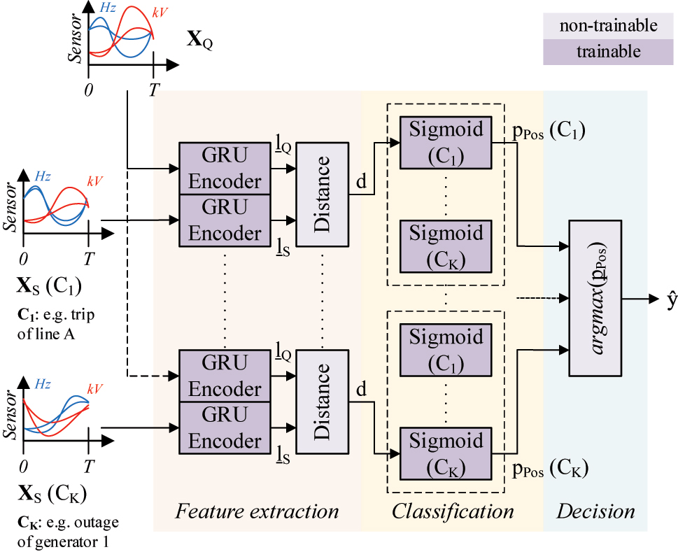
Siamese Sigmoid Network architecture.
SSNs estimate the class affiliation of a query instance
X
Q by the comparison with multiple support instances
X
S of known disturbance events C
1 … C
K. Therefore, a fixed number of support instances is selected for each class to create the support set S. Gated recurrent units (GRU) with additional attention mechanisms are used in the encoder network to compute the low-dimensional feature vectors
The weights
The difference between the positive and negative threshold distance corresponds to the margin
Depending on the classifier results, the two cases can arise:
the support and query instance belong to the same class if d → 0, p Pos → 1, and p Neg → 0, or
the support and query instance belong to different classes if d → ∞, p Pos → 0, and p Neg → 1.
With that, the class affiliation of the query instance
3.2 Benchmark models
The SSN model is compared with different benchmark models to evaluate the classification performance. The first benchmark model SSFD-SVM is a conventional disturbance classification approach from [27], which combines a strongest signal and fault detection (SSFD) algorithm for the localization task with a support-vector-machine (SVM) for the identification task. This approach requires a full PMU observability of the grid and is only applicable for closed-set classification problems. The second benchmark model Triplet-1NN is oriented at [28] and applies a triplet network architecture with hard negative online mining. This is a special training strategy for triplet networks and requires a sampling of negative examples beyond the margin. The feature vectors are generated with the same GRU encoder network as in Section 3.1 and the classification is performed with a 1-nearest-neighbor method (1NN). A full PMU observability is not required but again this approach is only applicable for closed-set classification problems. To solve open-set classification tasks, the third benchmark model GRU-DOC combines the GRU encoder network from Section 3.1 with a deep-open classifier (DOC) from [29]. Like the second benchmark model, a full PMU observability is not required.
3.3 Evaluation metrics
The classification models are evaluated for different classification tasks considering known and unknown disturbance events. For that, the class configuration of the K known classes will be extended with an additional container class C
U, which includes the rejections of the samples of all unknown classes, such that
the classification accuracy of the known classes η ACC,K,
the classification accuracy of the known and unknown classes η ACC,
the F1-score with macro averaging of the known classes η F1,K, and
the F1-score with macro averaging of the known and unknown classes η F1.
Thus, the true positives of the unknown classes are excluded from the calculations of η ACC and η F1. The macro averaged F1-score corresponds to the arithmetic mean of the class-specific F1-scores.
4 Simulation studies
4.1 Simulation model and database
As already described in [26], a generic power transmission system is simulated to extract the PMU frequency and voltage magnitude signals at all 400 kV busbars. The power system model includes 21 substations and 68 transmission lines with additional voltage regulators, power system stabilizers and protection systems. In total, the available database consists of 440 simulated contingencies at 7 operational points (OP1 to OP7) with different generation and load conditions. These operational points result from optimal power flow calculations and are given in Table 2. The grid topology is shown in Figure 4. The following disturbance types are considered within this study:
base load power plant outages (BLPP),
peak load plant outages (PLPP),
low (<50 % of the maximum capacity) and high (>50 % of the maximum capacity) load losses (LL Low and LL High ),
low (<50 % of the maximum capacity) and high (>50 % of the maximum capacity) PV losses (PV Low and PV High ),
line trips (L), and
short circuits at 10 % (SC 10), 50 % (SC 50), and 90 % (SC 90) line length.
Overview of the operational points.
| OP | Conventional | Renewable | Load |
|---|---|---|---|
| generation | generation | ||
| OP1 | 1512 MW | 1075 MW | 3060 MW |
| OP2 | 1355 MW | 1258 MW | 2900 MW |
| OP3 | 1066 MW | 1353 MW | 2834 MW |
| OP4 | 1104 MW | 1230 MW | 2527 MW |
| OP5 | 1619 MW | 1135 MW | 2839 MW |
| OP6 | 1121 MW | 1247 MW | 2679 MW |
| OP7 | 783 MW | 1198 MW | 2475 MW |

Topology of the simulated power system.
For the experiments, we considered 54 known and 60 unknown disturbance events with randomly chosen disturbance types and locations in the grid. We sampled the PMU frequency and voltage signals at the substations with a fixed window size T of 50 timesteps and a reporting rate of 25 f.p.s. from the 10 s post-disturbance records.
4.2 Test scenarios
To evaluate the influence of the nuisance variables on the disturbance classification results, we define the test scenarios listed in Table 3. For each scenario, we distinguish between a limited (“a”) and a full (“b”) observability of the grid with PMUs. In the “a”-scenarios the input signals are taken from 13 randomly selected PMUs of the grid. In the “b”-scenarios the input signals are taken from all 21 PMUs in the grid. Scenarios S.1a and S.1b investigate the influence of additional measurement noise with 20 dB and an AR-coefficient of AR = 0.2 in the test data. The measurement noise is generated by an autoregressive error model from [31]. Scenarios S.2a and S.2b investigate the influence of unknown operational points and scenarios S.3a and S.3b investigate the influence of unknown disturbance events in the test data. These unknown disturbance events correspond to new combinations of known disturbance types at known or unknown disturbance locations. Scenarios S.4a and S.4b include all nuisance variables.
Overview of the test scenarios.
| Scenario | PMUs | Training/validation data | Test data |
|---|---|---|---|
| S.1a | 13 | Classes: 54 (known) Operational points: OP2, OP3, OP4, OP6, OP7 Noise: – | Classes: 54 (known) Operational points: OP2, OP3, OP4, OP6, OP7 Noise: 20 dB with AR = 0.2 |
| S.1b | 21 (all) | Classes: 54 (known) Operational points: OP2, OP3, OP4, OP6, OP7 Noise: – | Classes: 54 (known) Operational points: OP2, OP3, OP4, OP6, OP7 Noise: 20 dB with AR = 0.2 |
| S.2a | 13 | Classes: 54 (known) Operational points: OP2, OP3, OP4, OP6, OP7 Noise: – | Classes: 54 (known) Operational points: OP1, OP5 Noise: – |
| S.2b | 21 (all) | Classes: 54 (known) Operational points: OP2, OP3, OP4, OP6, OP7 Noise: – | Classes: 54 (known) Operational points: OP1, OP5 Noise: – |
| S.3a | 13 | Classes: 54 (known) Operational points: OP2, OP3, OP4, OP6, OP7 Noise: – | Classes: 54 (known) and 60 (unknown) Operational points: OP2, OP3, OP4, OP6, OP7 Noise: – |
| S.3b | 21 (all) | Classes: 54 (known) Operational points: OP2, OP3, OP4, OP6, OP7 Noise: – | Classes: 54 (known) and 60 (unknown) Operational points: OP2, OP3, OP4, OP6, OP7 Noise: – |
| S.4a | 13 | Classes: 54 (known) Operational points: OP2, OP3, OP4, OP6, OP7 Noise: – | Classes: 54 (known) and 60 (unknown) Operational points: OP1, OP5 Noise: 20 dB with AR = 0.2 |
| S.4b | 21 (all) | Classes: 54 (known) Operational points: OP2, OP3, OP4, OP6, OP7 Noise: – | Classes: 54 (known) and 60 (unknown) Operational points: OP1, OP5 Noise: 20 dB with AR = 0.2 |
4.3 Results and discussion
The experimental results for the different test scenarios correspond to the average values of the 10-fold cross-validation runs after hyper-parameter tuning. We used early stopping as regularization technique. Table 4 shows the accuracies and F1-scores of the classification models SSN, Triplet-1NN, and GRU-DOC for the scenarios S.1a and S.1b. Due to the limited PMU observability in the “a”-scenarios, the SSFD-SVM benchmark model is only applied for the “b”-scenarios (see also Section 3.2). As it can be seen, the accuracy values and F1-scores decrease between roughly between −4 % and −5 % due to the measurement noise in the test data. In case of a limited PMU observability (scenario S.1a), the SSN model achieves the highest test accuracies (93.19 %) and test F1-scores (93.05 %) compared to the Triplet-1NN and GRU-DOC benchmark models. In case of a full PMU observability (scenario S.2b), the accuracy and F1-score results increase slightly among all models due to the higher number of input signals. Here, the SSN model again achieves the highest test accuracies (95.15 %) and F1-scores (94.98 %). In contrast to that, the SSFD-SVM benchmark model performs very poorly with a test accuracy of 80.77 % and a F1-score of 81.76 %. Also, the loss of accuracy and F1-score is significantly higher with roughly −7.5 % compared to the other models, which indicates a bad generalization capability of the model.
Performance results for the scenarios S.1a and S.1b.
| Model | η ACC,K in % (training) | η F1,K in % (training) | η ACC,K in % (test) | η F1,K in % (test) | Δη ACC,K in % | Δη F1,K in % |
|---|---|---|---|---|---|---|
| Scenario: S.1a | ||||||
| SSN | 98.17 | 98.11 | 93.19 | 93.05 | −4.98 | −5.06 |
| Triplet-1NN | 97.09 | 96.88 | 91.95 | 91.82 | −5.14 | −5.06 |
| GRU-DOC | 96.17 | 95.32 | 92.11 | 90.79 | −4.06 | −4.53 |
| Scenario: S.1b | ||||||
| SSN | 99.20 | 99.18 | 95.15 | 94.98 | −4.05 | −4.20 |
| Triplet-1NN | 99.47 | 99.40 | 94.88 | 94.83 | −4.59 | −4.57 |
| GRU-DOC | 96.55 | 96.01 | 92.37 | 91.53 | −4.18 | −4.48 |
| SSFD-SVM | 88.32 | 89.25 | 80.77 | 81.76 | −7.55 | −7.49 |
-
Bold values indicate the best performance results.
Table 5 shows the accuracies and F1-scores of the classification models SSN, Triplet-1NN, GRU-DOC, and SSFD-SVM for the scenarios S.2a and S.2b. In this case, the accuracy and F1-score decrease significantly of about −20 % to −50 % compared to the training results due to the new operational points. For the scenario S.2a, the Triplet-1NN benchmark model achieves the highest test accuracy (77.01 %) and test F1-score (75.38 %). For all models, the accuracy value decrease on average of about −20.66 % and the F1-score values of about −23.43 % compared to the training results. The accuracy and F1-score losses far exceed the results of the scenarios S.1a and S.1b (see Table 4), which shows a greater impact of unknown operational points on the classification performance compared to measurement noise. In case of scenario S.2b, the SSN model achieves the highest test accuracy (81.48 %) and the lowest accuracy and F1-score losses compared to the training results. The Triplet-1NN benchmark model still achieves the highest test F1-score (78.28 %). Again, the accuracies and F1-scores of the SSFD-SVM benchmark model are significantly lower compared to all other models, with a remarkably large difference between the training and test results.
Performance results for the scenarios S.2a and S.2b.
| Model | η ACC,K in % (training) | η F1,K in % (training) | η ACC,K in % (test) | η F1,K in % (test) | Δη ACC,K in % | Δη F1,K in % |
|---|---|---|---|---|---|---|
| Scenario: S.2a | ||||||
| SSN | 98.71 | 98.73 | 76.99 | 73.73 | −21.72 | −25.00 |
| Triplet-1NN | 97.26 | 97.01 | 77.01 | 75.38 | −20.25 | −21.63 |
| GRU-DOC | 95.24 | 92.67 | 75.23 | 69.01 | −20.01 | −23.66 |
| Scenario: S.2b | ||||||
| SSN | 98.75 | 98.64 | 81.48 | 77.65 | −17.27 | −20.99 |
| Triplet-1NN | 99.43 | 99.37 | 80.38 | 78.27 | −19.05 | −21.10 |
| GRU-DOC | 95.33 | 93.95 | 77.01 | 71.49 | −18.32 | −22.46 |
| SSFD-SVM | 88.01 | 88.99 | 33.83 | 37.73 | −54.18 | −51.26 |
-
Bold values indicate the best performance results.
In case of the scenarios S.3a and S.3b, we also evaluate the accuracies and F1-scores for the known and unknown classes. The corresponding training and test results are given in Table 6. Due to the missing rejection capability, the Triplet-1NN and the SSFD-SVM benchmark models cannot be applied for these scenarios (see also Section 3.2). As it can be seen, the additional integration of unknown classes in the test data significantly reduces the accuracy results η ACC and F1-score results η F1. A direct comparison between the η ACC,K and η ACC values or the η F1,K and η F1 values is difficult due to the different class configurations. Still, the high number of misclassifications in the test data demonstrates the high impact of unknown disturbance events on the overall classification performance. The SSN model outperforms the GRU-DOC benchmark model in both scenarios and achieves the highest accuracies (81.09 % for known classes and 58.32 % for all classes) and F1-scores (78.99 % for known classes and 57.27 % for all classes).
Performance results for the scenarios S.3a and S.3b.
| Model | η ACC,K in % (training) | η F1,K in % (training) | η ACC,K in % (test) | η ACC in % (test) | η F1,K in % (test) | η F1 in % (test) |
|---|---|---|---|---|---|---|
| Scenario: S.3a | ||||||
| SSN | 88.09 | 85.54 | 81.09 | 58.32 | 78.99 | 57.27 |
| GRU-DOC | 84.48 | 81.21 | 78.05 | 46.65 | 74.42 | 52.48 |
| Scenario: S.3b | ||||||
| SSN | 89.69 | 87.14 | 84.56 | 62.50 | 81.95 | 60.64 |
| GRU-DOC | 84.88 | 82.99 | 81.04 | 50.68 | 77.76 | 56.20 |
-
Bold values indicate the best performance results.
The results regarding the influence of all nuisance variables is given in Table 7. Similar to the scenarios S.3a and S.4b, the SSN model outperforms the GRU-DOC benchmark model and achieves the highest accuracies (77.65 % for known classes and 56.93 % for all classes) and F1-scores (74.91 % for known classes and 51.82 % for all classes). The large differences between the training and test results indicate the impact of the nuisance variables on the performance of the classification models.
Performance results for the scenarios S.4a and S.4b.
| Model | η ACC,K in % (training) | η F1,K in % (training) | η ACC,K in % (test) | η ACC in % (test) | η F1,K in % (test) | η F1 in % (test) |
|---|---|---|---|---|---|---|
| Scenario: S.4a | ||||||
| SSN | 88.11 | 85.14 | 77.65 | 56.93 | 74.91 | 51.82 |
| GRU-DOC | 82.83 | 79.29 | 72.43 | 44.39 | 67.51 | 46.52 |
| Scenario: S.4b | ||||||
| SSN | 89.92 | 87.68 | 80.03 | 59.72 | 77.07 | 54.35 |
| GRU-DOC | 85.60 | 83.53 | 75.23 | 48.01 | 71.28 | 49.84 |
-
Bold values indicate the best performance results.
5 Summary and outlook
This paper investigates the robustness of PMU based disturbance classification methods in case of deviations between the training and test data sets. For this, the classification problem is described from a systems theory point of view by introducing the nuisance variables: measurement noise, unknown operational points, and unknown disturbance events. Siamese Sigmoid Networks (SSN) as recurrent neural network based classification model are evaluated and compared to several closed-set and open-set benchmark models. A generic 400 kV transmission power system is modeled to simulate disturbance events under different operational conditions and to create the necessary training and test data sets. An autoregressive error model adds measurement noise to the test signals. The experiments show that SSNs perform on pair compared to Triplet networks in case of unknown operational points and achieve slightly better test results in case of measurement noise. Furthermore, SNNs clearly outperform an open-set classifier when handling unknown disturbance events. Especially unknown operational points and unknown disturbance events lead to severe performance degradations (above −20 % of accuracy and F1-score) in all classification models in the application phase. This demonstrates the importance of investigations regarding the robustness of disturbance classification models as well as possible improvements of the model performance under real conditions.
No field measurements from real power systems are available for this work but should be investigated in further studies to validate the approach. Future work should focus on an improved evaluation of the nuisance variables, especially model errors, and the derivation of representative datasets as well as performance criteria to develop robust disturbance classification models. Other benchmark models and benchmark power systems should be taken into consideration to further substantiate the findings. Also, the application of the disturbance classification in distribution systems (e.g. at 110 kV voltage level) could be investigated in future studies.
About the authors

André Kummerow, M. Sc., is a research associate at Fraunhofer IOBS-AST. Main research areas: Application of machine learning methods for monitoring energy networks, communication and IT security in energy networks.

Univ.-Prof. Dr.-Ing. Peter Bretschneider is a professor at the Faculty of Electrical Engineering and Information Technology for the subject area of energy use optimization at the TU Ilmenau and head of the Energy Department of Fraunhofer IOSB-AST. Main research interests: Energy management, time series analysis and forecasting, optimization and operation management in power grids, smart grids and energy markets.
-
Author contributions: All the authors have accepted responsibility for the entire content of this submitted manuscript and approved submission.
-
Research funding: None declared.
-
Conflict of interest statement: The authors declare no conflicts of interest regarding this article.
References
[1] C. Liu, S. McArthur, and S.-J. Lee, “Remedial action schemes and defense systems,” in Smart Grid Handbook, Chichester, UK, John Wiley & Sons, Ltd, 2016, pp. 1–10.10.1002/9781118755471.sgd032Suche in Google Scholar
[2] A. Kummerow, C. Brosinsky, C. Monsalve, S. Nicolai, P. Bretschneider, and D. Westermann, “PMU-based online and offline applications for modern power system control centers in hybrid AC-HVDC transmission systems,” in Proceedings of International ETG Congress 2019, 2019, pp. 405–410.Suche in Google Scholar
[3] C. Brosinsky, A. Kummerow, A. Naumann, A. Krönig, S. Balischewski, and D. Westermann, “A new development platform for the next generation of power system control center functionalities for hybrid AC-HVDC transmission systems,” in IEEE Power & Energy Society General Meeting, 2017, pp. 1–5.10.1109/PESGM.2017.8274090Suche in Google Scholar
[4] A. Phadke, M. Pai, A. Stankovic, and J. Thorp, Synchronized Phasor Measurements and Their Applications, New York, NY; Heidelberg, Springer, 2008.10.1007/978-0-387-76537-2Suche in Google Scholar
[5] N. Sharma, A. Tiwari, K. Verma, and S. Singh, “Applications of phasor measurement units (PMUs) in electric power system networks incorporated with FACTS controllers,” Int. J. Eng. Sci. Technol., vol. 3, no. 3, p. 19, 2011. https://doi.org/10.4314/ijest.v3i3.68423.Suche in Google Scholar
[6] Y. Chen, L. Xie, and P. Kumar, “Power system event classification via dimensionality reduction of synchrophasor data,” in IEEE 8th Sensor Array and Multichannel Signal Processing Workshop (SAM), 2014, pp. 57–60.10.1109/SAM.2014.6882337Suche in Google Scholar
[7] Y. Ge, A. Flueck, D.-K. Kim, J.-B. Ahn, J.-D. Lee, and D.-Y. Kwon, “Power system real-time event detection and associated data archival reduction based on synchrophasors,” IEEE Trans. Smart Grid, vol. 6, no. 4, pp. 2088–2097, 2015. https://doi.org/10.1109/tsg.2014.2383693.Suche in Google Scholar
[8] M. Biswal, Y. Hao, P. Chen, S. Brahma, H. Cao, and P. Leo, “Signal features for classification of power system disturbances using PMU data,” in 19th Power Systems Computation Conference, 2016, pp. 1–7.10.1109/PSCC.2016.7540867Suche in Google Scholar
[9] A. Singh and M. Fozdar, “Supervisory framework for event detection and classification using wavelet transform,” in IEEE PES General Meeting, 2017, pp. 1–5.10.1109/PESGM.2017.8274283Suche in Google Scholar
[10] A. Mathew and M. Aravind, “PMU based disturbance analysis and fault localization of a large grid using wavelets and list processing,” in Proceedings of the 2016 IEEE Region 10 Conference (TENCON), 2016, pp. 879–883.10.1109/TENCON.2016.7848131Suche in Google Scholar
[11] J. Ma, Y. Makarov, R. Diao, P. Etingov, J. Dagle, and E. Tuglie, “The characteristic ellipsoid methodology and its application in power systems,” IEEE Trans. Power Syst., vol. 27, no. 4, pp. 2206–2214, 2012. https://doi.org/10.1109/tpwrs.2012.2195232.Suche in Google Scholar
[12] G. Gajjar and S. Soman, “Auto detection of power system events using wide area frequency measurements,” in Eighteenth National Power Systems Conference (NPSC), 2014, pp. 1–6.10.1109/NPSC.2014.7103879Suche in Google Scholar
[13] D. Nguyen, R. Barella, S. Wallace, X. Zhao, and X. Liang, “Smart grid line event classification using supervised learning over PMU data streams,” in Sixth International Green and Sustainable Computing Conference, 2015, pp. 1–8.10.1109/IGCC.2015.7393695Suche in Google Scholar
[14] O. Dahal, H. Cao, S. Brahma, and R. Kavaseri, “Evaluating performance of classifiers for supervisory protection using disturbance data from phasor measurement units,” in IEEE PES Innovative Smart Grid Technologies Conference Europe (ISGT-Europe), 2014, pp. 1–6.10.1109/ISGTEurope.2014.7028892Suche in Google Scholar
[15] S. Fries and C.-P. Rückemann, “Finding needles in a haystack: line event detection on smart grid PMU data streams,” in The Sixth International Conference on Smart Grids, vol. 6, Green Communications and IT Energy-Aware Technologies, 2016, p. 6.Suche in Google Scholar
[16] R. Yadav, A. Pradhan, and I. Kamwa, “Real-time multiple event detection and classification in power system using signal energy transformations,” IEEE Trans. Ind. Inf., vol. 15, pp. 1521–1531, 2018. https://doi.org/10.1109/tii.2018.2855428.Suche in Google Scholar
[17] P. E. A. Cardoso, Deep Learning Applied to PMU Data in Power Systems, Porto, Portugal, Faculdade de Engenharia, 2016.Suche in Google Scholar
[18] W. Wang, H. Yin, C. Chen, et al.., “Frequency disturbance event detection based on synchrophasors and deep learning,” IEEE Trans. Smart Grid, vol. 4, pp. 3593–3605, 2020. https://doi.org/10.1109/tsg.2020.2971909.Suche in Google Scholar
[19] Y. Zhu, C. Liu, and K. Sun, “Image embedding of PMU data for deep learning towards transient disturbance classification,” in IEEE International Conference on Energy Internet (ICEI), 2018, pp. 169–174.10.1109/ICEI.2018.00038Suche in Google Scholar
[20] K. Mahapatra, S. Lu, A. Sengupta, and N. R. Chaudhuri, “Power system disturbance classification with online event-driven neuromorphic computing,” IEEE Trans. Smart Grid, vol. 12, no. 3, p. 11, 2021.10.1109/TSG.2020.3043782Suche in Google Scholar
[21] T. Athay, R. Podmore, and S. Virmani, “A practical method for the direct analysis of transient stability,” IEEE Trans. Power Appar. Syst., vol. 2, pp. 573–584, 1979. https://doi.org/10.1109/tpas.1979.319407.Suche in Google Scholar
[22] S. Brahma, R. Kavasseri, H. Cao, N. R. Chaudhuri, T. Alexopoulos, and Y. Cui, “Real-time identification of dynamic events in power systems using PMU data, and potential applications—models, promises, and challenges,” IEEE Trans. Power Delivery, vol. 32, pp. 294–301, 2017. https://doi.org/10.1109/tpwrd.2016.2590961.Suche in Google Scholar
[23] A. Kummerow, M. Dirbas, C. Monsalve, and P. Bretschneider, “Siamese Sigmoid Networks for the open classification of grid disturbances in power transmission systems,” IET Smart Grid, vol. 7, no. 1, pp. 11–146, 2022. https://doi.org/10.1049/stg2.12083.Suche in Google Scholar
[24] A. Kummerow, M. Dirbas, C. Monsalve, S. Nicolai, and P. Bretschneider, “Robust disturbance classification in power transmission systems with denoising recurrent autoencoders,” Sustain. Energy, Grids Netw., vol. 32, no. 15, p. 10, 2022. https://doi.org/10.1016/j.segan.2022.100803.Suche in Google Scholar
[25] A. Kummerow, C. Monsalve, and P. Bretschneider, “Siamese recurrent neural networks for the robust classification of grid disturbances in transmission power systems considering unknown events,” IET Smart Grid, vol. 5, pp. 11–61, 2021. https://doi.org/10.1049/stg2.12051.Suche in Google Scholar
[26] A. Kummerow, C. Monsalve, S. Nicolai, and P. Bretschneider, “Simultaneous online identification and localization of disturbances in power transmission systems,” in IEEE PES Innovative Smart Grid Technologies Europe (ISGT-Europe), 2019, pp. 1–5.10.1109/ISGTEurope.2019.8905711Suche in Google Scholar
[27] M. Biswal, S. M. Brahma, and H. Cao, “Supervisory protection and automated event diagnosis using PMU data,” IEEE Trans. Power Delivery, vol. 31, no. 4, pp. 1855–1863, 2016. https://doi.org/10.1109/tpwrd.2016.2520958.Suche in Google Scholar
[28] F. Schroff, D. Kalenichenko, and J. Philbin, “FaceNet: a unified embedding for face recognition and clustering,” in IEEE Conference on Computer Vision and Pattern Recognition (CVPR), 2015, pp. 815–823.10.1109/CVPR.2015.7298682Suche in Google Scholar
[29] L. Shu, H. Xu, and B. Liu, “DOC: deep open classification of text documents,” in Proceedings of the 2017 Conference on Empirical Methods in Natural Language Processing, 2017, pp. 2911–2916.10.18653/v1/D17-1314Suche in Google Scholar
[30] C. Geng, S.-J. Huang, and S. Chen, “Recent advances in open set recognition: a survey,” arXiv, 2018.Suche in Google Scholar
[31] A. Kummerow, M. Dirbas, C. Monsalve, S. Nicolai, and P. Bretschneider, “Influence of autoregressive noise on phasor data based disturbance classification,” in International Conference on Smart Energy Systems and Technologies (SEST), 2021, pp. 1–6.10.1109/SEST50973.2021.9543278Suche in Google Scholar
© 2023 the author(s), published by De Gruyter, Berlin/Boston
This work is licensed under the Creative Commons Attribution 4.0 International License.
Artikel in diesem Heft
- Frontmatter
- Editorial
- Selected contributions from the Workshop “Computational Intelligence”
- Methods
- Latin hypercubes for constrained design of experiments for data-driven models
- Handling of time delays in system identification with regularized FIR models
- Applications
- A fully automated touch-response behavior inspection pipeline on zebrafish larvae
- Approximative Modellierung eines LLC-Resonanzwandlers mit Takagi-Sugeno-Modellen
- Influence of nuisance variables on the PMU-based disturbance classification in power transmission systems
- Two-stage quality monitoring of a laser welding process using machine learning
- Fast power tracking control of PV power plants for frequency support
- Persönliches
- Prof. Dr.-Ing. habil. Joachim Rudolph zum 60. Geburtstag