A method for the use of ellipticities and spot diameters for the measurement of aberrations in wide-field telescopes
-
Lothar Noethe
 ,
Pietro Schipani
,
Pietro Schipani

Abstract
In wide-field survey telescopes, the patterns of spot sizes and ellipticities can be used to determine wavefront aberrations generated by the telescope. The calculation of spot sizes and ellipticities generated by telescope aberrations is most conveniently done if the aberrations are expressed in terms of Zernike-type polynomials whose derivatives are orthonormal. The field dependence of the spot sizes and ellipticities generated by the telescope can conveniently be expressed by low-order Zernike polynomials. Because the exposure times in astronomical survey work are typically rather short, this information may be used for a quasi-closed loop control of the telescope optics. The ability to accurately subtract ellipticities generated by telescope errors could also be useful for observations such as gravitational lensing surveys.
7 Appendix
7.1 Notations used for Zernike polynomials Zm, j and slope Zernike polynomials Sm, j
Correspondence between indices m, j, the Noll notation and commonly used names for Zernike polynomials.
| m | j | Noll notation | Name |
|---|---|---|---|
| 0 | 1 | Z1 | Piston |
| 0 | 2 | Z4 | Defocus |
| 0 | 3 | Z11 | Spherical aberration |
| 1 | 1 | Z2, Z3 | Tilt |
| 2 | 2 | Z7, Z8 | Third-order coma |
| 3 | 3 | Z16, Z17 | Fifth-order coma |
| 2 | 1 | Z5, Z6 | Third-order astigmatism |
| 2 | 2 | Z12, Z13 | Fifth-order astigmatism |
| 3 | 1 | Z9, Z10 | Trefoil |
7.2 Relationships between normalized and non-normalized Zernike and slope Zernike polynomials
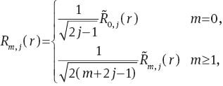
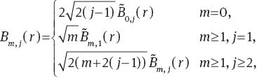
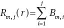
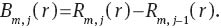
If modified radial components Rm,j(r) and Bm,j(r) are defined by:
the relationships between Zernike and slope Zernike polynomials are given by:
With n=m+2(j–1), the functions Rm,j(r) and Bm,j(r) are identical to the functions
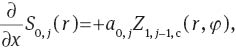
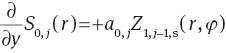
7.3 Expression of the derivatives of slope Zernike polynomials in terms of Zernike polynomials
The derivative of a slope Zernike polynomial Sm,j,a(r, φ) with respect to x and y can be expressed as a single Zernike polynomial Z1,j,a(r, φ) for m=0 or as a sum of two Zernike polynomials Zm,j,b(r, φ) and Zm+1,j-1,b(r, φ) for m>0, with a, b∈{c, s}.

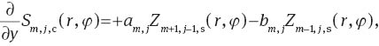


The values for the coefficients am,j and bm,j are shown in Table 5.
Coefficients used in Eqs. (66) to (71).
| m | c, s | j | ∂/∂x, ∂/∂y | am,j | bm,j |
|---|---|---|---|---|---|
| 0 | c, s | >1 | ∂/∂x, ∂/∂y | 0 | |
| 1 | c | 1 | ∂/∂x | 0 | 1 |
| 1 | ∂/∂y | 0 | 0 | ||
| >1 | ∂/∂x | 1/2 | |||
| >1 | ∂/∂x | 1/2 | 0 | ||
| 1 | s | 1 | ∂/∂x | 0 | 0 |
| 1 | ∂/∂y | 0 | 1 | ||
| >1 | ∂/∂x | 1/2 | 0 | ||
| >1 | ∂/∂y | 1/2 | |||
| >1 | c, s | 1 | ∂/∂x, ∂/∂y | 0 | |
| >1 | ∂/∂x, ∂/∂y | 1/2 | 1/2 |
7.4 Examples of ellipticity patterns due to telescope aberrations
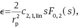
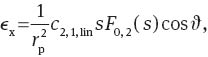
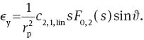
7.4.1 Linear astigmatism and defocus due to tilt of focal plane
A linear astigmatism that is symmetric to the x-axis and a linear defocus generated by a tilt of the focal plane around the y-axis are described by:
and by Eq. (29) with ϑ0,2=0, respectively. Similarly to Section 4.7 one obtains the following expressions:
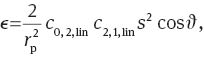

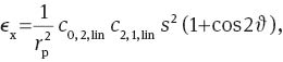
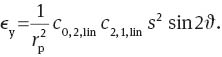
Because the dependence on the radial field variable s is proportional to s2, the field dependencies can be expressed in terms of Zernike polynomials Z0,1,c(s), Z0,2,c(s) and Z2, 1, c(s, ϑ) for ϵx and Z2,1,s(s, ϑ) for ϵy.
7.4.2 Linear astigmatism and nominal defocus
A linear astigmatism that is symmetric to the x-axis is described in Eq. (72) and a rotationally symmetric nominal defocus by:
Then,

The dependencies of the expressions on the field radius s can be expressed as polynomials with odd powers of s. Therefore, the field dependencies of the x- and y-components of
7.4.3 Trefoil and coma
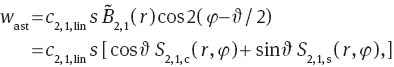
In the VST, nominal trefoil is negligible. However, the coefficient c3,1,c of field-constant S3,1,c(r, φ) in the VST may be of the order of 300 nm. Together with nominal third-order coma S1,2(r, φ), it may generate ellipticities of the order of 8ϵWL with the field dependencies:
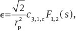

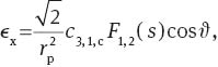
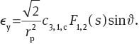
Because F1,2(s) is a polynomial in s with only odd powers, ϵx can be expressed by Zernike polynomials Z1,j,c(s, ϑ) and ϵy by Zernike polynomials Z1,j,s(s, ϑ).
References
[1] M. Liang, V. Krabbendam, C. F. Claver, S. Chandrasekharan and B. Xin, Proc. SPIE 8444, Q8444Q-1-13 (2012).Search in Google Scholar
[2] M. Jarvis and B. Jain, arXiv:astro-ph/0412234 (2004).Search in Google Scholar
[3] M. Jarvis, P. Schechter and B. Jain, arXiv:astro-ph/0810.0027 (2008).Search in Google Scholar
[4] Z. Ma, G. Bernstein, A. Weinstein and M. Sholl, Publ. Astron. Soc. Pac., 120, 1307–1317 (2008).Search in Google Scholar
[5] L. B. Moore, A. M. Hvisc and J. Sasian, Opt. Exp. 20, 15655–15670 (2008).Search in Google Scholar
[6] A. Manuel and J. Burge, Proc. SPIE 7433, 7433A (2009).Search in Google Scholar
[7] P. Schechter and R. Levinson, PASP 123, 812 (2011).10.1086/661111Search in Google Scholar
[8] K. Thompson, Adv. Opt. Techn. 2, 89–95 (2013).Search in Google Scholar
[9] C. A. Laury-Micoulout, A&A 51, 343 (1976).10.1007/BF02568162Search in Google Scholar
[10] W. Lukosz, Opt. Acta 10, 1–19 (1963).Search in Google Scholar
[11] J. Braat, J. Opt. Soc. Am. 4, 643–650 (1987).Search in Google Scholar
[12] I. W. Kwee and J. J. M. Braat, Pure Appl. Opt. 2, 21–32 (1993).Search in Google Scholar
[13] P. Schipani, M. Capaccioli, C. Arcidiacono, J. Argomedo, M. Dall’Ora, et al., Proc. SPIE 8444, 84441C (2012).Search in Google Scholar
[14] L. Noethe, Prog. Opt. 43, 1–69 (2002).Search in Google Scholar
[15] P. Schipani, L. Noethe, C. Arcidiacono, J. Argomedo, M. Dall’Ora, et al., J. Opt. Soc. Am. A29, 1359 (2012).10.1364/JOSAA.29.001359Search in Google Scholar PubMed
©2014 THOSS Media & De Gruyter Berlin/Boston
Articles in the same Issue
- Frontmatter
- Community
- News from the European Optical Society
- Conference Notes
- Conference Calendar
- Topical Issue: Optics for Astronomy / Guest Editors: Jan Burke, Andrew Rakich and Jim Burge
- Editorial
- Optics for astronomy – Editorial
- Review Articles
- Active optics with a minimum number of actuators
- Highly sensitive telescope designs for higher contrast observations
- Replicated spectrographs in astronomy
- Ultra-smooth finishing of aspheric surfaces using CAST technology
- Hydroxide catalysis bonding for astronomical instruments
- Research Articles
- Fabrication and metrology of lithium niobate narrowband optical filters for the solar orbiter
- A method for the use of ellipticities and spot diameters for the measurement of aberrations in wide-field telescopes
- Deflectometric measurement of large mirrors
- The Four-Laser Guide Star Facility: Design considerations and system implementation