Infinite energy harmonic maps from quasi-compact Kähler surfaces
-
Georgios Daskalopoulos


Abstract
We construct infinite energy harmonic maps from a quasi-compact Kähler surface with a Poincaré-type metric into an NPC space. This is the first step in the construction of pluriharmonic maps from quasiprojective varieties into symmetric spaces of non-compact type, Euclidean and hyperbolic buildings and Teichmüller space.
1 Introduction
In this paper, we prove the existence of harmonic maps of possibly infinite energy from quasi-compact Kähler surfaces with a Poincare-type metric to NPC spaces. Infinite energy harmonic maps between manifolds previously appeared in the work of Lohkamp and Wolf. Lohkamp [1] proved the existence of a harmonic map in a given homotopy class of maps between two non-compact manifolds, provided that a certain simplicity condition near infinity of the domain is satisfied. Wolf [2] studied harmonic maps of infinite energy when the domain is a nodal Riemann surface and applied it to describe degenerations of surfaces in the Riemann moduli space (see also [3]). A few years later, Jost and Zuo (cf. [4], [5]) sketched a proof of the existence of infinite energy maps from non-compact Kähler manifolds. The purpose of this paper is to provide a complete proof of the existence of harmonic maps from quasi-compact Kähler surfaces to a certain class of NPC targets. This is the first step in the construction of pluriharmonic maps from quasiprojective varieties into symmetric spaces of non-compact type, Euclidean and hyperbolic buildings and Teichmüller space which will be dealt in our upcoming paper, (cf. [6]).
Theorem 1
Let M,
ρ is proper (cf. Definition 2.7).
ρ(π 1(M)) satisfies Property (⋆) defined in Section 2.4.
Many interesting examples satisfy Property (⋆). These include homomorphisms into semisimple algebraic groups defined over
Remark 1.1
We will also prove logarithmic energy estimates near infinity (cf. Theorem 6.6 and Theorem 6.7). This means that, for any transverse holomorphic disk to the divisor, the energy density behaves
The main idea of the proof of Theorem 1 is to construct a prototype map which almost minimizes energy near infinity. This map is used to construct a Dirichlet solution defined on a compact subset of the domain. Because of the energy control, the sequence of harmonic maps corresponding to a compact exhaustion converges to an infinite energy harmonic map defined on the whole surface. This idea goes back to Lohkamp [1]. In our situation, the normal bundle of the divisor Σ may be non-trivial and the divisor may consist of more than one irreducible component. In other words, a quasi-compact Kähler surface
In [4], Jost and Zuo sketched a construction of harmonic maps from quasi-projective manifolds. The point of this paper is to provide the details of this argument for a quasi-compact Kähler surface. We felt that a careful presentation of this argument is necessary because all the constructions in our future papers (e.g. [6]) depend on this result.
In a remarkable paper, Mochizuki [7] proved the existence of pluriharmonic metrics on flat vector bundles over quasi-projective manifolds of any dimension. These metrics correspond to pluriharmonic maps into the symmetric space
One of our main applications of the existence of pluriharmonic maps is the construction of logarithmic symmetric differential forms over quasi-project manifolds. Using this, we prove a logarithmic version of a conjecture by Esnault in the linear case [6].
We provide an outline of the paper below.
In Section 3, we discuss neighborhoods of the divisor and a Poincaré-type metric g (cf. Definition 3.4) due to Cornalba and Griffiths [12]. This is a complete metric which puts the divisor at infinity.
In Section 4, we construct a prototype section
In Section 5, we give precise estimates for energy growth of the prototype section near the divisor at infinity. These are important because they imply the estimates for the harmonic section.
In Section 6, we use the prototype section
In Section 7, we sketch a proof in the case of higher dimensional quasi-compact Kähler manifolds. Note that in our upcoming papers, we will only use the two-dimensional case and this is why we gave the details only for Kähler surface domains.
2 Preliminaries
2.1 NPC spaces
We refer to [13] for more details.
Definition 2.1
A curve
Definition 2.2
An NPC space
where Q t = c(tl).
Notation 2.3
It follows immediately from Definition 2.2 that, given
Definition 2.4
Let
2.2 Maps into NPC spaces
In this paper, we consider harmonic maps into NPC spaces. Important examples are when the target space
where (Ω, g) is a Riemannian domain and dvol g is the volume form of Ω.
In the case when the target is an arbitrary NPC space, we use the following definition of energy due to Korevaar-Schoen. We refer to [14] for more details.
Let (Ω, g) be a bounded Lipschitz Riemannian domain. Let Ω ϵ be the set of points in Ω at a distance least ϵ from ∂Ω. Let B ϵ (x) be a geodesic ball centered at x and S ϵ (x) = ∂B ϵ (x). We say f: Ω → X is an L 2-map (or that f ∈ L 2(Ω, X)) if
For f ∈ L 2(Ω, X), define
where σ x,ϵ is the induced measure on S ϵ (x). We define a family of functionals
We say f has finite energy (or that f ∈ W 1,2(Ω, X)) if
It is shown in [14] that if f has finite energy, the measures e ϵ (x)dvol g converge weakly to a measure which is absolutely continuous with respect to the Lebesgue measure. Therefore, there exists a function e(x), which we call the energy density, so that e ϵ (x)dvol g ⇀ e(x)dvol g . In analogy to the case of smooth targets, we write |∇f|2(x) in place of e(x). In particular, the (Korevaar-Schoen) energy of f in Ω is
Definition 2.5
We say a continuous map
For V ∈ ΓΩ where ΓΩ is the set of Lipschitz vector fields on Ω, |f *(V)|2 is similarly defined. The real valued L 1 function |f *(V)|2 generalizes the norm squared on the directional derivative of f. The generalization of the pull-back metric is the continuous, symmetric, bilinear, non-negative and tensorial operator
where
We refer to [14] for more details.
Let (x 1, …, x n ) be local coordinates of (Ω, g) and g = (g ij ), g −1 = (g ij ) be the local metric expressions. Then energy density function of f can be written (cf. [14, (2.3vi)])
Next assume (Ω, g) is a 2-dimensional Hermitian domain and let (z
1 = x
1 + ix
2, z
2 = x
3 + ix
4) be local complex coordinates. We extend π
f
linearly cover
and
Thus,
2.3 Isometries of an NPC space
Throughout this paper, we denote the group of isometries of an NPC space
Definition 2.6
For
denote its translation length and define
The isometry I is elliptic if Δ
I
= 0 and
Definition 2.7
Let Γ be a finitely generated group, Λ be a finite set of generators of Γ,
We say ρ is proper if the sublevel sets of the function δ are bounded in
Remark 2.8
If
2.4 Property (⋆)
Given a homomorphism
Every I ∈ ρ(π 1(M)) has exponential decay to its translation length. In other words, either
I is semisimple, or
I is parabolic, fixes
For any commuting pair of isometries I 1, I 2 ∈ ρ(π 1(M)), either
I 1, I 2 do not fix a common point of
I 1, I 2 fix a common point
Remark 2.9
Let G be a semisimple algebraic group defined over
Lemma 2.10
Let C be a closed convex set in
Proof
Since I◦π(x), I −1◦π◦I(x) ∈ C, the definition of π implies
Thus, d(I(x), π◦I(x)) = d(I(x), I◦π(x)) which implies π◦I(x) = I◦π(x). □
Lemma 2.11
Let γ
1 and γ
2 be generators of the abelian group
such that
Proof
Assume that (i) of the second bullet point holds. Then by [15, Theorem 2.2.1 and Corollary 1.5.3), there exists a totally geodesic ρ-equivariant map
Thus, the map
Next, assume that (ii) of the second bullet point holds. Define
as follows: Fix t ∈ [0, ∞). For θ ∈ [0, 2π), let
2.5 Equivariant maps and sections of the associated flat
X
̃
-bundle
Following Donaldson [8], we will replace equivariant maps with sections of an associated fiber bundle. Assume we have the following:
a complete Riemannian manifold (M, g) with universal covering
an NPC space
an action of π 1(M) on
a homomorphism
Definition 2.12
A map
Remark 2.13
Assume
The quotient under the action of π
1(M) of the product
In other words,
is called the flat
There is a one-to-one correspondence between sections of this fibration and ρ-equivariant maps
satisfying the relationship
Since the energy density function
We can similarly define the pullback inner product and directional energy density functions of f by using the corresponding notions for
Furthermore, for sections f 1, f 2, we define
where
2.6 Harmonic maps from punctured Riemann surfaces
In this paper, many of the constructions will depend on harmonic maps for punctured Riemann surfaces. Below, we summarize the results of the paper [10], [11].
Let
Fix
For a given section
Recall that d(f(z), f 0(z)) is defined by (2.2).
Definition 2.14
We say a section
By the triangle inequality, this definition is independent of the choice of
where
Definition 2.15
For a homomorphism
We record our result in [6], [7].
Theorem 2.16
(Existence and Uniqueness of the Dirichlet solution on
Furthermore, there exists a constant C > 0 that depends only on
u has sub-logarithmic growth.
3 The Poincaré-type metric and its estimates
3.1 Neighborhoods near the divisor
This subsection closely follows [7]. We let
Furthermore, let
where {Σ
j
} is the set of irreducible components of Σ. Let σ
j
be the canonical section of
We denote by
For clarity, we will also denote the unit disk by
To study a neighborhood of the juncture, let P ∈ Σ
i
∩Σ
j
for some i, j ∈ {1, …, L} with i ≠ j, and let V
P
be a neighborhood of P containing no other crossings. Choose holomorphic trivializations e
i
(resp. e
j
) of
For each j = 1, …, L, let h
j
be a Hermitian metric on
The metric h is the Euclidean metric in a neighborhood V P of every crossing P, i.e.
(3.2)By rescaling σ 1 and σ 2 if necessary, we can assume without the loss of generality that
(3.3)The metric h induces the orthogonal decomposition
(3.4)the restriction of h to NΣ j is same as h j .
For r ∈ (0, 1], we set
There exists r > 0 such that the restriction of the exponential map
defines diffeomorphism of
Denote
The restriction of NΣ
j
→ Σ
j
to
We also identity
We denote by
We now consider a finite collection of sets near the divisor of the following two types:
A set of type (A) admits a local unitary trivialization
(3.9)of
A set of type (B) is as in (3.3); i.e.
(3.10)where V P be an open set containing a single crossing P ∈ Σ i ∩Σ j (i ≠ j). By the property (i) of the hermitian metric h, (z 1, z 2) are holomorphic coordinates with respect to
(3.11)is a local unitary trivialization of
Definition 3.1
We will refer to the coordinates (z
1, z
2) discussed in (A) above as the standard product coordinates on a set
Definition 3.2
We will refer to the coordinates (z
1, z
2) discussed in (B) above as the standard product coordinates and the holomorphic coordinates on a set
Remark 3.3
Holomorphic coordinates in a set of type (A) are defined later (cf. Definition 3.6).
3.2 Poincaré-type metric
Recall the Poincaré metric
Using the canonical section
Definition 3.4
Let
By scaling
Definition 3.5
Fix j and define on
Define
Below we derive some estimates for the metric g in a set of type (A) and of type (B) (See (3.9) and (3.10) for definitions of a set of type (A) and (B)). These are an expanded form of the estimates derived by Mochizuki [7].
3.3 Metric estimates in set of type (A)
Let
Fix a local trivialization e of
With σ
j
the canonical section of
Thus, ζ is holomorphic with respect to
Definition 3.6
We refer to
as the holomorphic coordinates (with respect to
Since z
2 = 0 = ζ on Ω × {0} and z
2 ≠ 0, ζ ≠ 0 on
Taking real and imaginary parts,
Let
be a smooth function bounded above and bounded away from 0 satisfying
Thus,
Plugging in
From this, we immediately obtain
This implies
where
The function a depends on the choice of e and σ whereas the function b depends on the choice of e and h j . Thus, by scaling σ if necessary, we can assure that b satisfies the following two conditions:
We compute
Note that because of (3.18) and since b is a smooth function bounded away from 0, we have
where
and
In coordinate z
1 of Ω ⊂ Σ
j
, let the local expression of the metric
Furthermore, the local expression for the inverse g −1 is
The product metric P on
The inverse P −1
Thus,
Comparing the local expression of g and P, we obtain
A straightforward computation gives
The metric P (and hence the metric g) is of finite volume over
Moreover, since
there exists a constant C > 0 such that
Lemma 3.7
The Poincaré type metric g defined by Definition 3.4 satisfies the following: There exists c > 0 such that, on the set
Proof
This is immediate from the fact that the metric
Remark 3.8
The key feature of the metric P is the following: Define Q to be the product metric
Then
This is important in Section 5 below where we estimate the energy of v. In particular, we have
Note that the inside integral on the right hand side above is exactly the energy of the harmonic map
3.4 Metric estimates in a set of type (B)
First recall that a type (B) set of Section 3.1 is a set
such that the standard product coordinates (z
1, z
2) are also holomorphic coordinates with respect to complex structure
In the coordinates (z 1, z 2) and with ρ = |z 1| and r = |z 2|, the local expression of the metric P associated to the above Kähler form is
and the inverse P −1 is given by
With
Thus,
A straightforward computation gives
Similarly to (3.30), we also obtain for subsets
Lemma 3.9
The Poincaré type metric g of Definition 3.4 satisfies the following: There exists c > 0 such that in neighborhood
Proof
This is immediate from (3.36). □
4 The prototype section
The goal of this section is to construct a prototype section with logarithmic energy growth near the divisor. The key is the fiber-wise harmonic sections on the normal bundle of the divisor Σ, the existence of which follows from the Dirichlet problem on the punctured disk (cf. Theorem 2.16).
Recall the sets of type (A) and of type (B) described in (3.9) and (3.10) respectively. In Section 4.1 and Section 4.2, we construct a local prototype section in a set of type (A) and (B) respectively. In Section 4.3, we glue these sections together to define a prototype section near the divisor and extend it to all of M. In summary, we construct a locally Lipschitz global section
of logarithmic energy growth near the divisor.
4.1 In a neighborhood away from the junctures
The goal of this subsection is to construct a local prototype section in a set of type (A) and derive some energy estimates. We start with the following:
(z 1, z 2) are the standard product coordinates of
r, θ are parameters defined by z 2 = re iθ
4.1.1 Construction of a prototype section in a set of type (A)
We define
by setting v to be the fiber-wise harmonic section with boundary values given by
is the unique harmonic section with logarithmic energy growth and boundary values
4.1.2 Derivative estimates in a set of type (A)
Lemma 4.1
(Derivative estimates in set of type (A)). There exists a constant C such that
where
Proof
Denote the Lipschitz constant of k on
By Theorem 2.16 (iii) and the triangle inequality,
Thus,
In other words, for every fixed
4.2 In a neighborhood of the juncture
The goal of this subsection is to construct a local prototype section in a set of type (B) and derive some derivative estimates. We start with the following:
(z 1, z 2) are the standard product (and holomorphic) coordinates
ρ, ϕ, r, θ are the parameters defined by z 1 = ρeiϕ and z 2 = re iθ
κ is the restriction of
4.2.1 Construction of a prototype section in a set of type (B)
We construct the local section
In what follows, we will assume that
By Property (⋆) and Lemma 2.11, for each t ∈ [0, ∞), there exist constants a, b > 0 (by modifying the constants a, b from Lemma 2.11) and a section
satisfying
(4.3)Define the diagonal set
Define v D : D → X as follows: Fix
For
For
be the geodesic between
where we use γ ρ to also denote the section
Let
and
be a homeomorphism defined by (see Figure 1)
Define
by setting v 1 to be the fiber-wise harmonic section with boundary values given by
is the unique harmonic section with boundary values
Similarly, let
and
be the homeomorphism defined by
We define
by setting v 2 to be the fiber-wise harmonic section with boundary values given by
Let
be the section defined by
Note that v is well defined since Z 1 ∩ Z 2 = D and
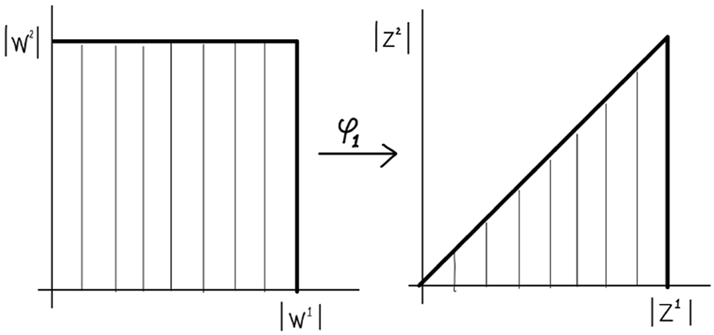
The map φ 1.
4.2.2 Derivative estimates in a set of type (B)
On Z 1, since z 1 = w 1 and z 2 = |w 1|w 2, we have
By (4.3),
Thus, noting that w 1 = z 1 = ρeiϕ ,
Furthermore, (4.3) implies
Since v
1 is a fiber-wise harmonic section, an argument analogous to the proof of first inequality of Lemma 4.1 (i.e. apply the maximum principle for subharmonic functions
Thus,
Since κ is a Lipschitz map, v
D
◦φ
1 is a Lipschitz section for
Furthermore, using the harmonicity of v
1 restricted to the slice
for
Lemma 4.2
(Derivative estimates in a set of type (B) away from the juncture).
For
where
Proof
Since
Lemma 4.3
(Derivative estimates in a set of type (B) near the juncture).
For v restricted to
for
Proof
We only prove the first estimate, the second being similar. First, note that the lower bound follows from the definition of
for
If
After a change of variables z 1 = |w 2|w 1, z 2 = w 2,
Thus, we have
Finally, if
4.3 Gluing the maps
Given the homomorphism
Let P = {0} × {0} ∈ Σ
j
∩Σ
i
and
The identification of the product space
(cf. (3.11)).
Recall the following items associated with the set
Next, let
The identification
of the bundle
By [14, Proposition 2.6.1], there exists a locally Lipschitz section
be the local prototype section defined in Section 4.2. The composition of v
U
and the quotient map
Also let k
V
be the lift to
be the local prototype section defined in Section 4.1.1. The composition of v
V
and the quotient map
We claim that we can glue these local sections together to define v in U ∪ V. To do so, we have to show the following.
Lemma 4.4
If U and V are sets of type (B) and (A) respectively, then the sections v U and v V agree on U* ∩ V*.
Proof
For
Indeed, since multiplication by τ(p) ∈ U(1) is a conformal map, v
V,p
◦τ(p) is harmonic on
Similar construction holds for two sets of type (A).
Lemma 4.5
If U and V are both of type (A) and U ∩ V ≠ ∅, then v U and v V agree on U* ∩ V*.
Proof
Apply the same argument as Lemma 4.4. □
Let
and extend to the rest of M as a well-defined, locally Lipschitz global section of
Definition 4.6
The map
constructed above is called the prototype section. The corresponding ρ-equivariant map
5 Energy estimates of the prototype section
The goal of this section is to obtain the energy estimates of the prototype section
of Definition 4.6 with respect to the Poincaré-type metric g given by Definition 3.4. Throughout this section, we use C to denote constants that are independent of the distance to the divisor. (Note that C may change from line to line.)
We consider the following three types of sets intersecting the divisor
Subsets of a set of type (B).
A neighborhood of Σ can be covered by a finite collection of sets of the above type. In order to estimate the energy of v, we will compute its energy in each such set.
5.1 Energy in a set of type (A)
In this subsection we will use the following notation in addition to the one used in Section 4.1.
P is the product metric on
Note that
The strategy for estimating the energy of the prototype section v in
Lemma 5.1
For a subset
Proof
By (3.29),
hence the inequality on the right follows from Lemma 4.1 (cf. Remark 3.8).
By the definition of
which proves the inequality on the left. □
Lemma 5.2
For a subset
Proof
By Lemma 5.1, it suffices to show that the difference of the energy of v with respect to g and with respect to P is bounded; i.e.
We obtain the above estimate with the help of Lemma 5.15 found in the Appendix to this chapter. Therefore we need to first show that the assumption (5.3) of Lemma 5.15 is satisfied; in other words, we need an estimate of the integral of
First, to bound the z
1-energy of v, we use estimate
Second, from [6, 7, Proof of Lemma 3.4], we have
Thus, Lemma 5.1 and the identities for
We set
Noting that
where the constant C′ depends only on C.
We use the above estimate to compute the difference between
To bound this term, note that since by (3.28)
and
and thus
Thus,
which in turn implies
To bound this term, note that since
by (3.29). Combining the above, we obtain
Thus
The other terms of
Lemma 5.3
For a subset
for any locally Lipschitz section
Proof
Since
Thus, the desired estimate with g replaced by P follows from combining the above estimate with Lemma 5.1. Thus, we are left to show that
To do so, note that if the inequality
does not hold, then we are done since the desired estimate holds by Lemma 5.2. Hence, we can assume the above inequality and apply Lemma 5.15 to conclude
where the constant C′ depends only on C. The rest of the proof is exactly as in the proof of Lemma 5.1. □
5.2 Energy in a set of type (B) away from the crossing
In this subsection we will use the following notation in addition to the one used in Section 4.2.
P is the product metric on
Since
the metric expressions of g in a set of type (A) and of type (B) (cf. (3.24) and (3.32) respectively) show that g restricted to
Lemma 5.4
For a subset
Proof
Follow the proof of Lemma 5.1 but by replacing (3.29) by (3.36) and Lemma 4.1 by Lemma 4.2. (Note that
Lemma 5.5
For a subset
Lemma 5.6
For a subset
for any locally Lipschitz section
5.3 Energy in a set of type (B) at the crossing
In this subsection we will use the following notation in addition the one used in Section 4.2.
P is the product metric on
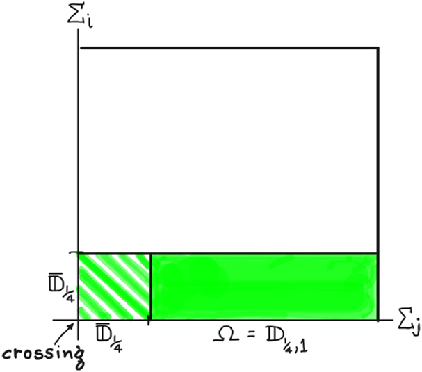
The goal is to estimate the energy of v in the set
pictured in Figure 3. The procedure for doing so involves an extra step compared to the procedure in the previous two subsections. Namely, we will first derive an expression for the energy with respect to the product metric P in the box
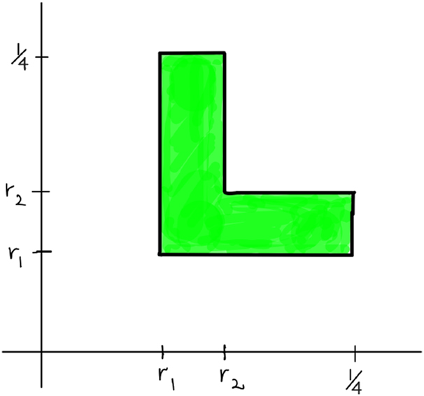
The region
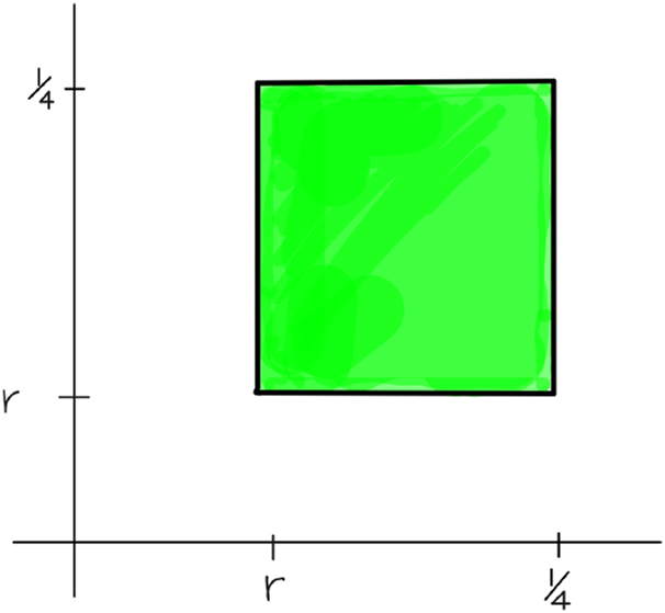
The region
Definition 5.7
We define
Remark 5.8
Note that
Lemma 5.9
In a subset
for
Proof
By Lemma 4.3,
for
Combining the above, we obtain
and similarly
□
Lemma 5.10
In a subset
the prototype section v satisfies
Proof
By a straightforward computation,
The second term is bounded by
Thus, combining the above equality and the inequality and then multiplying by
Similarly,
Furthermore, Lemma 5.9 implies
Thus, the desired estimate follows from the fact that
Lemma 5.11
In a subset
the prototype section v satisfies
Proof
Follows from the metric estimate (3.34) and Lemma 5.10. □
Lemma 5.12
In a subset
the prototype section v satisfies
for any locally Lipschitz section
Proof
Follow the proof of Lemma 5.3 using Lemma 5.11 instead of Lemma 5.2. □
5.4 Energy estimates for the prototype section near the divisor
Combining the results of the previous three subsections, we obtain the following estimate in an open set
Proposition 5.13
There exists a constant C > 0 such that the prototype section v of Definition 4.6 satisfies
Proof
Since we can cover a neighborhood of Σ by a finite collection of sets of type (A) and type (B), the estimate follows from Lemma 5.2, Lemma 5.5 and Lemma 5.11. □
Proposition 5.14
The section v is almost minimizing in M in the following sense: There exists a constant C > 0 such that
for any section
Proof
Since we can cover a neighborhood of Σ by a finite collection of sets of type (A) and type (B), the estimate, the estimate follows from Lemma 5.3, Lemma 5.6 and Lemma 5.12. □
5.5 Appendix
We conclude this chapter with the following calculus result which was used in the derivation of the energy estimates.
Lemma 5.15
Let
where
then
where C′ is a constant depending only on C and c.
Proof
We start with the following claim: For any function
To prove (5.4), first note that 2−i−1 ≤ r ≤ 2−i implies
Furthermore, by the assumption that ψ(r) ≥ c ≥ 0,
The above two inequalities imply
which proves (5.4).
Let
Since ψ(r) ≥ c, we have by (5.4) that
for a.e. z 1 ∈ Ω. Thus,
□
6 Harmonic maps of possibly infinite energy
The goal of this section is to prove Theorem 1, the existence of a harmonic map of logarithmic energy growth. In Section 6.1, we show the existence of a harmonic map with the help of the prototype map. In Section 6.2, we record the energy growth estimates for this map.
Throughout this section, we use C to denote constants that are independent of the parameter r. Note that C may change from line to line.
6.1 Proof of existence, Theorem 1
Proof
For
Next, let
be the energy minimizer among all sections that agree with v on ∂M r for each r ∈ (0, r 1]. The existence of such a section u r follows from the proof of [14, Theorem 2.7.2].
Since
we have that
The right hand side of the inequality (6.1) is independent of the parameter r; i.e. once we fix
Let
where Λ is the finite set of generators used in the definition of proper, Definition 2.7. If we let
then by equivariance
In other words,
Thus, following the proof of [15, Theorem 2.1.3], taking a compact exhaustion and applying the usual diagonalization argument, there exists a subsequence of
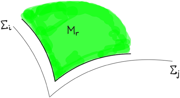
The region M r ⊂ M.
6.2 Energy estimates for the harmonic section
Lemma 6.1
For the harmonic section
Lemma 6.2
If
Proof
From the fact that
Proposition 5.14 implies
Combining the above two inequalities we obtain
and similarly
The desired estimate follows from the above two inequalities. □
Lemma 6.3
If
Proof
The estimate follows from Proposition 5.13 and Lemma 6.2. □
Lemma 6.4
If
where (z
1, z
2 = re
iθ
) are the standard product coordinates on
Proof
All the estimates except for the last two follow immediately from Lemma 6.3. The last two follow from the other estimates and Lemma 5.15. □
Recall that the standard product coordinates (z
1, z
2) on a set
Lemma 6.5
If (z
1, z
2 = re
iθ
) and (z
1, ζ = se
iη
) are the standard product coordinates and holomorphic coordinates respectively on a set
where a is a smooth function both bounded above and bounded away from 0 (cf. (3.18) and (3.19)).
Proof
Since
by (3.19), the first estimate follows immediately. Furthermore, differentiating the above with respect to ζ, we obtain the next two estimates. The last four estimates are obtained by evaluating the differential forms of (3.17) on the vector fields
Theorem 6.6
If
where (z
1, ζ = seiη
) are the holomorphic coordinates on
Proof
By Lemma 6.5, we have
Thus,
Thus, the second, third and fourth estimates now follow from Lemma 6.4. The first estimate is a restatement of the first estimate of Lemma 6.4. □
Theorem 6.7
If
where (z
1 = ρeiϕ
, z
2 = re
iθ
) are the holomorphic coordinates on
7 Generalization to higher dimensions
The construction of harmonic maps from quasi-compact Kähler surfaces generalizes to quasi-compact Kähler manifolds of arbitrary dimension. Indeed, let
In our upcoming papers, we will only use the two-dimensional case. More precisely, we combine Theorem 1 with an inductive argument due to Mochizuki (cf. [7]) to deduce the existence of pluriharmonic maps in any dimension in the quasi-projective case. This is why we gave the details only for Kähler surface domains.
Acknowledgments
The authors would like to thank Y. Deng, T. Mochizuki and Y. Siu for illuminating discussions.
-
Research ethics: Not applicable.
-
Author contributions: The authors have accepted responsibility for the entire content of this manuscript and approved its submission.
-
Competing interests: The authors state no conflict of interest.
-
Research funding: Georgios Daskalopoulos supported in part by NSF DMS-2105226 and a Simons collaboration grant, Chikako Mese supported in part by NSF DMS-2304697.
-
Data availability: Not applicable.
References
[1] J. Lohkamp, “An existence theorem for harmonic maps,” Manuscripta Math., vol. 67, no. 1, pp. 21–23, 1990, https://doi.org/10.1007/bf02568419.Search in Google Scholar
[2] M. Wolf, “Infinite energy harmonic maps and degeneration of hyperbolic surfaces in moduli spaces,” J. Diff. Geom., vol. 33, no. 2, pp. 487–539, 1991, https://doi.org/10.4310/jdg/1214446328.Search in Google Scholar
[3] S. Gupta and M. Wolf, “Quadratic differentials, half-plane structures, and harmonic maps to trees,” Comm. Math. Helv., vol. 91, no. 2, pp. 317–356, 2016, https://doi.org/10.4171/cmh/388.Search in Google Scholar
[4] J. Jost and K. Zuo, “Harmonic maps of infinite energy and rigidity results for representations of fundamental groups of quasi-projective varieties,” J. Diff. Geom., vol. 47, no. 3, pp. 469–503, 1997, https://doi.org/10.4310/jdg/1214460547.Search in Google Scholar
[5] K. Zuo, “Representations of fundamental groups of algebraic varieties,” in Lecture Notes in Mathematics, vol. 1708, Berlin, Heidelberg, Springer, 1999.10.1007/BFb0092569Search in Google Scholar
[6] D. Brotbek, G. Daskalopoulos, Y. Deng and C. Mese. “Pluriharmonic maps into buildings and symmetric differentials.” arXiv:2206.11835.Search in Google Scholar
[7] T. Mochizuki, “Asymptotic behaviour of tame harmonic bundles and an application to pure twistor D-modules,” Memoirs AMS, vol. 185, no. 870, p. 0, 2007, https://doi.org/10.1090/memo/0870.Search in Google Scholar
[8] S. Donaldson, “Twisted harmonic maps and the self-duality equations,” Proc. London Math. Soc., vol. 55, no. 1, pp. 127–131, 1987, https://doi.org/10.1112/plms/s3-55.1.127.Search in Google Scholar
[9] K. Corlette, “Archimedian superrigidity and hyperbolic geometry,” Ann. Math., vol. 135, no. 1, pp. 165–182, 1990, https://doi.org/10.2307/2946567.Search in Google Scholar
[10] G. Daskalopoulos and C. Mese, “Notes on harmonic maps.” Preprint arXiv:2301.04190.Search in Google Scholar
[11] G. Daskalopoulos and C. Mese, “Infinite energy harmonic maps from Riemann surfaces to CAT(0) spaces,” J. Geom. Anal.10.1515/ans-2023-0122Search in Google Scholar
[12] M. Cornalba and P. Griffiths, “Analytic cycles and vector bundles on noncompact algebraic varieties,” Invent. Math., vol. 28, no. 1, pp. 1–106, 1975, https://doi.org/10.1007/bf01389905.Search in Google Scholar
[13] M. R. Bridson and A. Haefliger, Metric Spaces of Non-positive Curvature, Berlin, Springer-Verlag, 1999.10.1007/978-3-662-12494-9Search in Google Scholar
[14] N. Korevaar and R. Schoen, “Sobolev spaces and harmonic maps for metric space targets,” Comm. Anal. Geom., vol. 1, no. 4, pp. 561–659, 1993, https://doi.org/10.4310/cag.1993.v1.n4.a4.Search in Google Scholar
[15] N. Korevaar and R. Schoen, “Global existence theorem for harmonic maps to non-locally compact spaces,” Comm. Anal. Geom., vol. 5, no. 2, pp. 333–387, 1997.10.4310/CAG.1997.v5.n2.a4Search in Google Scholar
© 2024 the author(s), published by De Gruyter, Berlin/Boston
This work is licensed under the Creative Commons Attribution 4.0 International License.
Articles in the same Issue
- Frontmatter
- Editorial
- Preface for the special issue in honor of Joel Spruck
- Research Articles
- A C 2,α,β estimate for complex Monge–Ampère type equations with conic sigularities
- On subsolutions and concavity for fully nonlinear elliptic equations
- On the functional ∫Ωf + ∫Ω*g
-
On constant higher order mean curvature hypersurfaces in
- Annuloids and Δ-wings
- Comparison formulas for total mean curvatures of Riemannian hypersurfaces
- Infinite energy harmonic maps from quasi-compact Kähler surfaces
- Non-homogeneous fully nonlinear contracting flows of convex hypersurfaces
- Rigidity properties of Colding–Minicozzi entropies
- Stability and critical dimension for Kirchhoff systems in closed manifolds
- Eigenvalue lower bounds and splitting for modified Ricci flow
- A Liouville theorem for superlinear parabolic equations on the Heisenberg group
- Geometry of branched minimal surfaces of finite index
- Nonlinear problems inspired by the Born–Infeld theory of electrodynamics
- Perturbation compactness and uniqueness for a class of conformally compact Einstein manifolds