Uniform stabilization for a strongly coupled semilinear/linear system

Marcelo M. Cavalcanti; Valéria N. Domingos Cavalcanti; Dilberto da Silva Almeida Júnior; Victor Hugo Gonzalez Martinez; Mauro de Lima Santos

doi:10.1515/ans-2022-0017

Article Open Access

Uniform stabilization for a strongly coupled semilinear/linear system

Marcelo M. Cavalcanti , Valéria N. Domingos Cavalcanti , Dilberto da Silva Almeida Júnior , Victor Hugo Gonzalez Martinez and Mauro de Lima Santos

Published/Copyright: July 28, 2022

Published by

Become an author with De Gruyter Brill

Submit Manuscript Author Information Explore this Subject

From the journal Advanced Nonlinear Studies Volume 22 Issue 1

Abstract

In this manuscript, we analyze the exponential stability of a strongly coupled semilinear system of Klein-Gordon type, posed in an inhomogeneous medium Ω , subject to local dampings of different natures distributed around a neighborhood of the boundary according to the geometric control condition (GCC). The first one is of the type viscoelastic and is distributed around a neighborhood ω of the boundary ∂ Ω of Ω , according to the GCC. The second one is a frictional damping and we consider it hurting the GCC. The third dissipation, which acts only in the second equation (according to the GCC), is of the frictional type. We show that the energy of the system goes uniformly and exponentially to zero for all initial data of finite energy taken in bounded sets of finite energy phase space. We also prove the exponential decay for the linear problem associated with this same system, and in this case, no restrictions are made with respect to dimension of the space nor with respect to the limitation of the initial data in the phase space.

Keywords: wave equation; Klein-Gordon system; Kelvin-Voigt damping; frictional damping; exponential stability

MSC 2010: Primary: 35L05; Secondary: 35L53; 35B40; 93B07

1 Introduction

1.1 Description of the problem

This article addresses the exponential stability of a semilinear wave equation system posed in an inhomogeneous medium and subject to Kelvin-Voigt and frictional dampings locally distributed:

(1.1) ρ ( x ) u t t − div ( K ( x ) ∇ u ) + v 2 u − div ( a ( x ) ∇ u t ) + c ( x ) u t + ∑ j = 1 d ∂ x j ( γ ( x ) v t ) = 0 in Ω × R + , ρ ( x ) v t t − div ( K ( x ) ∇ v ) + u 2 v + b ( x ) v t + ∑ j = 1 d γ ( x ) ∂ x j u t = 0 in Ω × R + , u = v = 0 on ∂ Ω × R + , u ( x , 0 ) = u 0 ( x ) , u t ( x , 0 ) = u 1 ( x ) in Ω , v ( x , 0 ) = v 0 ( x ) , v t ( x , 0 ) = v 1 ( x ) in Ω ,

where Ω ⊂ R d , d ≤ 2 , is a bounded domain with smooth boundary Γ = ∂ Ω , ρ : Ω → R + , k i j : Ω → R , 1 ≤ i , j ≤ d are C ∞ ( Ω ) functions such that for all x ∈ Ω and ξ ∈ R d ,

(1.2) α 0 ≤ ρ ( x ) ≤ β 0 , k i j ( x ) = k j i ( x ) , α ∣ ξ ∣ 2 ≤ ξ ⊤ ⋅ K ( x ) ⋅ ξ ≤ β ∣ ξ ∣ 2 ,

where α 0 , β 0 , α , β are positive constants and K ( x ) = ( k i j ) i , j is a symmetric positive-definite matrix. We denote by ω , with smooth boundary ∂ ω , the intersection of Ω with a neighborhood of ∂ Ω in R d .

Assumption 1.1

The nonnegative functions a ( ⋅ ) and b ( ⋅ ) , responsible for the localized dissipative effect, satisfy the following conditions:

a ( ⋅ ) ∈ L ∞ ( Ω ) is a nonnegative function. In addition, there exists a compact, connected set A ⊂ Ω with smooth boundary and nonempty interior, verifying A ≔ { x ∈ Ω : a ( x ) = 0 } . We also assume that a ∈ C 0 ( ω ¯ ) , where ω ≔ Ω \ A .
b ( ⋅ ) ∈ C 0 ( Ω ¯ ) is a nonnegative function and b ( x ) ≥ b 0 > 0 in Ω ⧹ B where B ≔ { x ∈ A : d ( x , y ) > ε , y ∈ ∂ A } . We also assume that B is compact, connected, with smooth boundary and nonempty interior.
We assume that γ ∈ W 1 , ∞ ( Ω ) and 0 ≤ γ ( x ) ≤ a ( x ) and 0 ≤ γ ( x ) ≤ b ( x ) a.e. in Ω .

Assumption 1.2

c ( ⋅ ) ∈ C 0 ( Ω ¯ ) is a nonnegative function such that c ( x ) ≥ c 0 > 0 in a neighborhood of the boundary ∂ A of the set A ≔ { x ∈ Ω : a ( x ) = 0 } , according to Figure 1.

$Figure 1 The Kelvin-Voigt damping a ( x ) a\left(x) is positive in ω ≔ Ω \ A \omega \left:= \Omega \backslash A while the frictional damping c ( x ) c\left(x) is effective in a neighborhood of ∂ A \partial A , that is, c ( x ) ≥ c 0 > 0 c\left(x)\ge {c}_{0}\gt 0 in V ε / 2 = { x ∈ Ω : d ( x , y ) < ε / 2 , y ∈ ∂ A } {V}_{\varepsilon \text{/}2}=\left\{x\in \Omega :d\left(x,y)\lt \varepsilon \text{/}2,y\in \partial A\right\} for ε > 0 \varepsilon \gt 0 small enough.$

Figure 1

The Kelvin-Voigt damping a ( x ) is positive in ω ≔ Ω \ A while the frictional damping c ( x ) is effective in a neighborhood of ∂ A , that is, c ( x ) ≥ c 0 > 0 in V ε / 2 = { x ∈ Ω : d ( x , y ) < ε / 2 , y ∈ ∂ A } for ε > 0 small enough.

It is worth mentioning that if a ( x ) = 0 , for all x ∈ Ω , the frictional dampings b ( x ) and c ( x ) are not strong enough to provide the exponential and uniform decay of the energy, observe that in this case c ( x ) violates the geometric control condition (GCC), see [3,4]. However, the frictional damping c ( x ) plays a key role which we will describe next (Figures 2 and 3).

$Figure 2 Admissible geometry for the frictional dissipations b ( x ) b\left(x) .$

Figure 2

Admissible geometry for the frictional dissipations b ( x ) .

$Figure 3 Admissible geometries for the Kelvin-Voigt and frictional dissipations a ( x ) a\left(x) and c ( x ) c\left(x) , respectively.$

Figure 3

Admissible geometries for the Kelvin-Voigt and frictional dissipations a ( x ) and c ( x ) , respectively.

Let us assume that the following hypothesis is also satisfied:

Assumption 1.3

ω geometrically controls Ω , i.e., there exists T 0 > 0 , such that every geodesic of the metric G ( x ) , where G ( x ) = K ( x ) ρ ( x ) − 1 travelling with speed 1 and issued at t = 0 , intercepts ω in a time t < T 0 .

As in [6], Assumption 1.3 is the so-called GCC. It is well-known that it is necessary and sufficient for stabilization and control of the linear wave equation, see [3,4,7,8,14,28] and references therein. For this reason and since in the present article we do not have any control of the geodesics because of the inhomogeneous medium we consider ω a neighborhood of the whole boundary ∂ Ω and to give conditions on the metric G = ( K / ρ ) − 1 in order every geodesic of the metric G enters the set ω in a time t < T 0 . According to [6], this assumption is not fulfilled for every matrix G = ( K / ρ ) − 1 and it is possible to give concrete examples where this situation occurs for a broad class of Riemannian metrics.

According to [5], when we do not have any control on the geodesics of the metric G = ( K / ρ ) − 1 , we have to assume damping everywhere on Ω , satisfying the following assumptions:

for all x ∈ ∂ Ω , a ( x ) > 0 ;
for all geodesic t ∈ I ↦ x ( t ) ∈ Ω of the metric G = ( K / ρ ) − 1 , with 0 ∈ I , there exists t ≥ 0 such that a ( x ( t ) ) > 0 .

The best way to do this is by using the ideas introduced in Cavalcanti et al. [7,8], namely, a ( x ) ≥ a 0 in a neighborhood, ω , of the boundary ∂ Ω , while a ( x ) ≥ a 0 ∗ > 0 in ( Ω \ ω ) \ V , where V = ⋃ i = 1 k V i and meas ( V ) ≥ meas ( Ω \ ω ) − ε , for an arbitrary ε > 0 . In Figure 4, the demarcated region ω (in gray) and ( Ω \ ω ) \ V (in light gray) illustrate the damped region on the manifold ( Ω , G ) , which can be considered with measure as small as desired, however, totally distributed on Ω . The demarcated region V ≔ ⋃ i = 1 k V i (in white) illustrates the region without damping with measure arbitrarily large but also totally distributed in Ω .

Figure 4

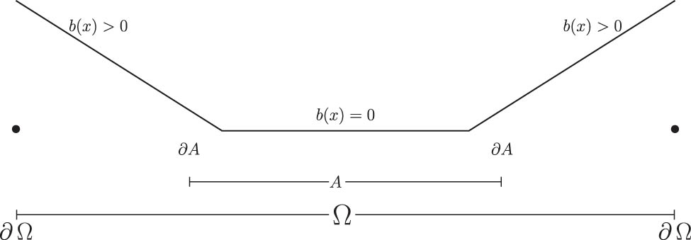
Totally distributed damping.

We observe that if G = I d condition (i) implies that (ii) holds since the geodesics are straight lines. On the other hand, for a general metric condition (i) can be verified without (ii) holds, if, for instance, G admits a trapped geodesic (Figure 5).

$Figure 5 In the left side G = I d G={I}_{d} and the geodesics are straight lines. a > 0 a\gt 0 on the blue region around the boundary. In the right side, there is a trapped geodesic that does not meet the damped area in blue which violates the GCC.$

Figure 5

In the left side G = I d and the geodesics are straight lines. a > 0 on the blue region around the boundary. In the right side, there is a trapped geodesic that does not meet the damped area in blue which violates the GCC.

One of the main ingredients for the stabilization of system (1.1) is a unique continuation principle, so we assume the following hypothesis:

Assumption 1.4

For every T ≥ T 0 , the only solution u , v ∈ C ( ] 0 , T [ ; L 2 ( Ω ) ) ∩ C ( ] 0 , T [ , H − 1 ( Ω ) ) to the system

(1.3) ρ ( x ) u t t − div ( K ( x ) ∇ u ) + V 1 ( x , t ) u = V 3 ( x , t ) v in Ω × ( 0 , T ) , ρ ( x ) v t t − div ( K ( x ) ∇ v ) + V 2 ( x , t ) v = V 3 ( x , t ) u in Ω × ( 0 , T ) , u = v = 0 on ω ,

where V 1 ( x , t ) , V 2 ( x , t ) , and V 3 ( x , t ) are elements of L ∞ ( ] 0 , T [ , L d + 1 2 ( Ω ) ) , is the trivial one u = v = 0 .

Remark 1.1

This type of condition in Assumption 1.4 is generally assumed in control/stabilization statements and the possibility to overcome it to every setting seems to be an open question. We observe that Proposition 2.2 of [10] gives an example where the unique continuation principle holds at least locally. For more details see [9,13,20,29].

We also emphasize that Kelvin-Voigt-type dissipation plays a fundamental role in the passings to the limits in the proof of our main result, due to the coupling term introduced in this article.

1.2 Main goal, methodology, and previous results

The main objective of the present manuscript is to prove the existence and uniqueness for weak solutions to problem (1.1) and, in addition, that those solutions decay exponentially and uniformly to zero, that is, setting

(1.4) E u , v ( t ) = 1 2 ∫ Ω ρ ( x ) ∣ u t ( x , t ) ∣ 2 + ρ ( x ) ∣ v t ( x , t ) ∣ 2 + ∇ u ( x , t ) ⊤ ⋅ K ( x ) ⋅ ∇ u ( x , t ) d x + 1 2 ∫ Ω ∇ v ( x , t ) ⊤ ⋅ K ( x ) ⋅ ∇ v ( x , t ) + ( u v ) 2 ( x , t ) d x ,

there exist positive constants C , γ , such that

(1.5) E u ( t ) ≤ C e − γ t E u ( 0 ) , for all t ≥ T 0 ,

for all weak solutions to problem (1.1), provided that the initial data { u 0 , v 0 , u 1 , v 1 } are taken in bounded sets of H 0 1 ( Ω ) × H 0 1 ( Ω ) × L 2 ( Ω ) × L 2 ( Ω ) . This result is a local stabilization result. Indeed, the constants C and γ are uniform on every ball in H 0 1 ( Ω ) × H 0 1 ( Ω ) × L 2 ( Ω ) × L 2 ( Ω ) with radius R > 0 of the energy space but the result does not guarantee that the decay rate is global one, i.e., whether (1.5) holds with constants C , γ which are independent of the initial data.

Inspired by Dehman et al. [13] or Dehman et al. [14] we give a direct proof of the inverse inequality to problem (1.1), namely, we prove that given T ≥ T 0 there exists a constant positive C = C ( T ) such that

(1.6) E u , v ( 0 ) ≤ C ∫ 0 T ∫ Ω a ( x ) ∣ ∇ u t ( x , t ) ∣ 2 + c ( x ) ∣ u t ( x , t ) ∣ 2 + b ( x ) ∣ v t ( x , t ) ∣ 2 d x d t ,

provided the initial data are taken in bounded sets of H 0 1 ( Ω ) × H 0 1 ( Ω ) × L 2 ( Ω ) × L 2 ( Ω ) .

To prove (1.6) and therefore the stability result, we argue by contradiction and we find a sequence of { w n , z n } of solutions to problem (1.1) such that E w n , z n ( 0 ) = 1 . In order to obtain a contradiction we are going to prove that E w n , z n ( 0 ) → 0 as n → + ∞ . We shall prove, by exploiting the properties of K ( x ) , a ( x ) , b ( x ) , c ( x ) and a unique continuation principle, that

(1.7) ∫ 0 T ∫ Ω ⧹ C ∣ w t n ∣ 2 d x d t → 0 and ∫ 0 T ∫ Ω ⧹ C ∣ z t n ∣ 2 d x d t → 0

when n goes to infinity, where C = { x ∈ A : d ( x , y ) > ε / 2 , y ∈ ∂ A } .

Our wish is to propagate the convergence (1.7) from Ω ⧹ C × ( 0 , T ) to the whole set Ω × ( 0 , T ) . In order to do this, we consider the microlocal defect measures μ 1 and μ 2 , associated with the kinetic component of solution of the linear wave equation.

First, we shall establish the convergence

(1.8) ρ ( x ) ∂ t 2 w t n − div ( K ( x ) ∇ w t n ) → 0 in H loc − 2 ( Ω × ( 0 , T ) ) , ρ ( x ) ∂ t 2 z t n − div ( K ( x ) ∇ z t n ) → 0 in H loc − 2 ( Ω × ( 0 , T ) ) ,

which is enough to ensure that the supp ( μ 1 ) and supp ( μ 2 ) are contained in the characteristic set of the wave operator. However, the last convergence is not sufficient for propagation, since we need a stronger convergence, namely,

ρ ( x ) ∂ t 2 w t n − div ( K ( x ) ∇ w t n ) → 0 in H loc − 1 ( Ω × ( 0 , T ) ) , ρ ( x ) ∂ t 2 z t n − div ( K ( x ) ∇ z t n ) → 0 in H loc − 1 ( Ω × ( 0 , T ) ) .

The problematic terms are precisely div ( a ( x ) ∇ w t n ) , − ∑ j = 1 d ∂ x j ( γ ( x ) z t n ) , and − ∑ j = 1 d γ ( x ) ∂ x j w t n because

∂ t ( div ( a ( x ) ∇ w t n ) ) → 0 strongly in H loc − 2 ( Ω × ( 0 , T ) ) , as n → + ∞ , ∂ t − ∑ j = 1 d ∂ x j ( γ ( x ) z t n ) → 0 strongly in H loc − 2 ( Ω × ( 0 , T ) ) , as n → and + ∞ ∂ t − ∑ j = 1 d γ ( x ) ∂ x j w t n → 0 strongly in H loc − 2 ( Ω × ( 0 , T ) ) , as n → + ∞ .

This is the moment that the frictional dissipation c ( x ) w t n plays a fundamental role in the collar of the boundary ∂ A . Indeed, note that a ( x ) ∇ w t m = − ∑ j = 1 d ∂ x j ( γ ( x ) z t n ) = 0 in A × ( 0 , T ) and − ∑ j = 1 d γ ( x ) ∂ x j w t n = 0 in B × ( 0 , T ) . Consequently, since

ρ ( x ) w t t n − div ( K ( x ) ∇ w n ) = − α n 2 ( z n ) 2 w n − c ( x ) w t n in A × ( 0 , T ) . ρ ( x ) z t t n − div ( K ( x ) ∇ z n ) = − α n 2 ( w n ) 2 z n − b ( x ) z t n in B × ( 0 , T ) .

Assuming for a moment that ( α n 2 ( z n ) 2 w n ) and ( α n 2 ( w n ) 2 z n ) converge to 0 in L 2 ( Ω × ( 0 , T ) ) as m → + ∞ , we will have that

□ w t n → 0 in H loc − 1 ( int A × ( 0 , T ) ) , as n → + ∞ , □ z t n → 0 in H loc − 1 ( int B × ( 0 , T ) ) , as n → + ∞ ,

from which we deduce that inside the sets int A × ( 0 , T ) and int B × ( 0 , T ) , μ 1 and μ 2 propagate along the bicharacteristic flow of this operator, which signifies, particularly, that if some point ω 0 = ( t 0 , x 0 , τ 0 , ξ 0 ) does not belong to the supp ( μ 1 ) or supp ( μ 2 ) the whole bicharacteristic issued from ω 0 is out of supp ( μ 1 ) or supp ( μ 1 ) , respectively. However, since supp ( μ 1 ) ⊂ C × ( 0 , T ) , supp ( μ 2 ) ⊂ B × ( 0 , T ) ⊂ C × ( 0 , T ) , and every geodesic starting in a point of C (resp. B ) enters in the set Ω ⧹ C (resp. Ω ⧹ B ). Consequently, from which we obtain that supp ( μ i ) = ∅ for i = 1 , 2 , and so, both w t n and z t n converge to zero in L loc 2 ( Ω × ( 0 , T ) ) . With some calculations we can show that

(1.9) lim n → ∞ ∫ 0 T ∫ Ω ∣ w t n ( x , t ) ∣ 2 d x d t = lim n → ∞ ∫ 0 T ∫ Ω ∣ z t n ( x , t ) ∣ 2 d x d t = 0 .

From convergence (1.9) and an argument of equipartition of energy, we can conclude that { E w n , z n ( 0 ) } converges to 0, as n → + ∞ , obtaining the desired contradiction. This will be clarified in Section 3.

The model proposed in this article is inspired by an equation introduced by Segal in [30], given by

(1.10) u t t − Δ u + m 1 2 u + g v 2 u = 0 in Ω × ( 0 , T ) , v t t − Δ v + m 2 2 v + h u 2 v = 0 in Ω × ( 0 , T ) ,

which describes the interaction of scalar fields u , v of mass m 1 , m 2 , respectively, with interaction constants g and h . This system defines the motion of charged mesons in an electromagnetic field. As the interest of this article is to make the mathematical analysis, there is no loss of generality if we consider only the case in which m 1 = m 2 = 0 and g = h = 1 .

For a complete literature review on systems similar to the one proposed in this article, see [6] and references therein, for example: [1,2,11,12,15,16, 17,18,22, 23,24,25, 26,28,32].

There are two main difficulties regarding problem (1.1). The nature of dissipations and coupling terms generate unbounded operators and the presence of the coefficients in the wave operators, as considered in the present article, makes the analysis much more refined in terms of the rays of the geometrical optics. Furthermore, the coupling term introduced in this article requires a Kelvin-Voigt dissipation and as is well known, this type of dissipation can cause instability of the system. The main ingredients in the proof are as follows: (i) a unique continuation principle for systems and (ii) the propagation of the microlocal defect measure by the geodesic flow.

This article is organized as follows. In Section 2, we give some notations and we establish the well-posedness to problem (1.1). In Section 3, we give the proof of the stabilization which consists our main result. In Section 4, we describe the result that establishes the exponential stability for the linear equation associated with problem (1.1). Finally, in the appendix we recall some basic results of microlocal analysis.

2 Well-posedness

We consider the weak phase space

ℋ = H 0 1 ( Ω ) × H 0 1 ( Ω ) × L 2 ( Ω ) × L 2 ( Ω ) ,

which is endowed with the inner product

⟨ ( u 1 , u 2 , u 3 , u 4 ) , ( v 1 , v 2 , v 3 , v 4 ) ⟩ ℋ = ∫ Ω ∇ u 1 ⊤ ⋅ K ( x ) ⋅ ∇ v 1 + ∇ u 2 ⊤ ⋅ K ( x ) ⋅ ∇ v 2 + ρ u 3 v 3 + ρ u 4 v 4 d x .

Denoting W ( t ) = ( u , v , u t , v t ) we may rewrite problem (1.1) as the following Cauchy problem in ℋ

(2.1) ∂ W ∂ t ( t ) = A W ( t ) + ℱ ( W ( t ) ) , W ( 0 ) = ( u 0 , v 0 , u 1 , v 1 ) ,

where the linear unbounded operator A : D ( A ) → ℋ is given by

(2.2) A = 0 0 I 0 0 0 0 I 1 ρ div ( K ( x ) ∇ ( ⋅ ) ) 0 1 ρ div ( a ( x ) ∇ ( ⋅ ) ) − 1 ρ c ( x ) I − 1 ρ ∑ j = 1 d ∂ x j ( γ ( x ) ( ⋅ ) ) 0 1 ρ div ( K ( x ) ∇ ( ⋅ ) ) − 1 ρ ∑ j = 1 d γ ( x ) ∂ x j ( ⋅ ) − 1 ρ b ( x ) I ,

that is,

(2.3) A ( u , v , w , z ) = w z 1 ρ div ( K ( x ) ∇ u + a ( x ) ∇ w ) − 1 ρ c ( x ) w − 1 ρ ∑ j = 1 d ∂ x j ( γ ( x ) z ) 1 ρ div ( K ( x ) ∇ v ) − 1 ρ ∑ j = 1 d γ ( x ) ∂ x j w − 1 ρ b ( x ) z ⊤

with domain

(2.4) D ( A ) = ( u , v , w , z ) ∈ ℋ : w , z ∈ H 0 1 ( Ω ) 1 ρ div ( K ( x ) ∇ u + a ( x ) ∇ w ) − 1 ρ ∑ j = 1 d ∂ x j ( γ ( x ) z ) ∈ L 2 ( Ω ) 1 ρ div ( K ( x ) ∇ v ) − 1 ρ ∑ j = 1 d γ ( x ) ∂ x j w − 1 ρ b ( x ) z ∈ L 2 ( Ω )

and ℱ : ℋ → ℋ is the nonlinear operator

(2.5) ℱ ( u , v , w , z ) = 0 , 0 , − 1 ρ v 2 u , − 1 ρ u 2 v .

Now, we are in conditions to state the well-posedness result for problem (2.1), which ensures that problem (1.1) is globally well-posed.

Theorem 2.1

(Global well-posedness) Assume that the hypotheses on ρ and K are fulfilled and the initial data ( u 0 , v 0 , u 1 , v 1 ) ∈ ℋ . Then problem (2.1) possesses a unique mild solution W ∈ C ( [ 0 , ∞ ) ; ℋ ) . Moreover, if ( u 0 , v 0 , u 1 , v 1 ) ∈ D ( A ) , then the solution is regular.

Proof

First of all the operator A : D ( A ) ⊂ ℋ → ℋ defined by (2.3) and (2.4) generates a C 0 -semigroup of contractions e A t on the energy space ℋ . Indeed, it is easy to see that for all ( u , v , w , z ) ∈ D ( A ) , we have

(2.6) ( A U , U ) = − ∫ Ω ( a ( x ) ∣ ∇ w ∣ 2 + c ( x ) ∣ w ∣ 2 + b ( x ) ∣ z ∣ 2 ) d x ≤ 0 ,

which shows that the operator A is dissipative. Next, we shall prove that 0 ∈ ρ ( A ) , where ρ ( A ) is the resolvent set of A proving the well-posedness for the linear problem associated by using the well-known Lumer-Phillips theorem. Indeed, for any given ( f , g , h , k ) ∈ ℋ , we solve the equation A ( u , v , w , z ) = ( f , g , h , k ) , which is recast on the following way:

(2.7) w = f ∈ H 0 1 ( Ω ) , z = g ∈ H 0 1 ( Ω ) , 1 ρ div ( K ( x ) ∇ u + a ( x ) ∇ w ) − 1 ρ c ( x ) w − 1 ρ ∑ j = 1 d ∂ x j ( γ ( x ) z ) = h ∈ L 2 ( Ω ) , 1 ρ div ( K ( x ) ∇ v ) − 1 ρ ∑ j = 1 d γ ( x ) ∂ x j w − 1 ρ b ( x ) z = k ∈ L 2 ( Ω ) .

From (2.7), we obtain

(2.8) w = f , z = g .

Substituting the equations of (2.8) in the last two equations of (2.7), we obtain

(2.9) 1 ρ div ( K ( x ) ∇ u ) = − 1 ρ div ( a ( x ) ∇ f ) + 1 ρ c ( x ) f + 1 ρ ∑ j = 1 d ∂ x j ( γ ( x ) g ) + h , 1 ρ div ( K ( x ) ∇ v ) = 1 ρ b ( x ) g + 1 ρ ∑ j = 1 d γ ( x ) ∂ x j f + k .

Equivalently,

(2.10) − div ( K ( x ) ∇ u ) = div ( a ( x ) ∇ f ) − c ( x ) f − ∑ j = 1 d ∂ x j ( γ ( x ) g ) − ρ h , − div ( K ( x ) ∇ v ) = − b ( x ) g − ∑ j = 1 d γ ( x ) ∂ x j f − ρ k .

Define

a ˜ : H 0 1 ( Ω ) × H 0 1 ( Ω ) × H 0 1 ( Ω ) × H 0 1 ( Ω ) ⟶ R

given by

(2.11) a ˜ ( ( u 1 , v 1 ) , ( u 2 , v 2 ) ) = ∫ Ω ( ∇ u 1 ) ⊤ ⋅ K ( x ) ⋅ ∇ u 2 + ( ∇ v 1 ) ⊤ ⋅ K ( x ) ⋅ ∇ v 2 d x .

Then, a ˜ ( ⋅ , ⋅ ) is bilinear, continuous, and coercive. From the Lax-Milgram theorem, given

( a 0 , b 0 ) = div ( a ( x ) ∇ f ) − c ( x ) f − ∑ j = 1 d ∂ x j ( γ ( x ) g ) − ρ h , − b ( x ) g − ∑ j = 1 d γ ( x ) ∂ x j f − ρ k ∈ ( H − 1 ( Ω ) ) 2 ,

there exists a unique ( u , v ) ∈ H 0 1 ( Ω ) × H 0 1 ( Ω ) , such that

a ˜ ( ( u , v ) , ( χ , η ) ) = ⟨ a 0 , χ ⟩ H − 1 ( Ω ) , H 0 1 ( Ω ) + ⟨ b 0 , η ⟩ H − 1 ( Ω ) , H 0 1 ( Ω ) for all ( χ , η ) ∈ H 0 1 ( Ω ) × H 0 1 ( Ω ) .

Taking χ ∈ C 0 ∞ ( Ω ) and η = 0 we deduce that

− div ( K ( x ) ∇ u ) = a 0 in D ′ ( Ω ) ,

and consequently,

− div ( K ( x ) ∇ u ) = a 0 in H − 1 ( Ω ) .

Proceeding in the same way, we deduce that

− div ( K ( x ) ∇ v ) = b 0 in H − 1 ( Ω ) .

From the above we deduce that ( u , v , w , z ) ∈ D ( A ) , since

(2.12) 1 ρ div ( K ( x ) ∇ u + a ( x ) ∇ w ) − 1 ρ ∑ j = 1 d ∂ x j ( γ ( x ) z ) = 1 ρ c ( x ) f + h ∈ L 2 ( Ω ) , 1 ρ div ( K ( x ) ∇ v ) − 1 ρ ∑ j = 1 d γ ( x ) ∂ x j w − 1 ρ b ( x ) z = k ∈ L 2 ( Ω ) ,

which gives us the desired solution.

Moreover, by multiplying the third line of (2.7) by u , the fourth line by v and integrating over Ω and combining the Young and Cauchy-Schwarz inequalities we find that there exists a constant C > 0 such that

‖ u ‖ H 0 1 ( Ω ) ≤ C ( ‖ f ‖ H 0 1 ( Ω ) + ‖ g ‖ H 0 1 ( Ω ) + ‖ h ‖ L 2 ( Ω ) )

and

‖ v ‖ H 0 1 ( Ω ) ≤ C ( ‖ f ‖ H 0 1 ( Ω ) + ‖ g ‖ H 0 1 ( Ω ) + ‖ k ‖ L 2 ( Ω ) ) .

It follows that

‖ A − 1 ( f , g , h , k ) ‖ ℋ = ‖ ( u , v , w , z ) ‖ ℋ ≤ C ‖ ( f , g , h , k ) ‖ ℋ ,

that is, A − 1 is a bounded operator densely defined, since D ( A − 1 ) = Im ( A ) = ℋ . Therefore, 0 ∈ ρ ( A ) . Then by the contraction principle, we easily obtain R ( λ I − A ) = ℋ for a sufficiently small λ > 0 .

Indeed, let G : ℋ ⟶ ℋ given by G U = A − 1 ( λ U − F ) , where F = ( f , g , h , k ) . Then, G is a contraction for λ > 0 sufficiently small. Indeed,

‖ G U − G V ‖ = ‖ A − 1 ( λ U − F ) − A − 1 ( λ V − F ) ‖ = ‖ λ A − 1 U − A − 1 F − λ A − 1 V + A − 1 F ‖ = ‖ λ A − 1 ( U − V ) ‖ ≤ λ ‖ A − 1 ‖ ‖ U − V ‖ .

Thus, for 0 < λ < 1 ‖ A − 1 ‖ , we have the desired. Therefore, the operator G admits a unique fix point, that is, there exist U ∈ ℋ such that A − 1 ( λ U − F ) = U . Consequently, U ∈ D ( A ) and ( λ I − A ) U = F .

This, together with the dissipativeness of A , implies that the density of D ( A ) in ℋ by Theorems 1.4.3, 1.4.5, and 1.4.6 in Pazy’s book [27]. Thus, A generates a C 0 semigroup of contractions on H by Lumer-Phillips theorem.

As in [6], it is easy to show that the nonlinear operator ℱ : ℋ → ℋ given in (2.5) is a locally Lipschitz continuous operator. Here, it is necessary the restriction on the dimension d . Hence by Theorems 6.1.4 and 6.1.5 in Pazy’s book [27], the Cauchy problem (1.1) has a unique mild solution

W ( t ) = e A t W ( 0 ) + ∫ 0 t e A ( t − s ) ℱ ( W ( s ) ) d s , for all t ∈ [ 0 , T max ) .

Let us see that T max = ∞ . Indeed, given the energy functional defined in (1.4), it follows that

d d t E u , v ( t ) = − ∫ Ω a ( x ) ∣ ∇ u t ( x , t ) ∣ 2 d x − ∫ Ω c ( x ) ∣ u t ( x , t ) ∣ 2 d x − ∫ Ω b ( x ) ∣ v t ( x , t ) ∣ 2 d x ,

which shows that E u , v ( t ) is nonincreasing with E u , v ( t ) ≤ E u ( 0 ) for all t ∈ [ 0 , T max ) . On the other hand, we have that

E u , v ( t ) ≥ 1 2 ∫ Ω ρ ( x ) ∣ u t ( x , t ) ∣ 2 + ρ ( x ) ∣ v t ( x , t ) ∣ 2 d x + 1 2 ∫ Ω ∇ u ( x , t ) ⊤ ⋅ K ( x ) ⋅ ∇ u ( x , t ) + ∇ v ( x , t ) ⊤ ⋅ K ( x ) ⋅ ∇ v ( x , t ) d x = 1 2 ‖ ( u , v , u t , v t ) ‖ ℋ 2 .

Thus,

1 2 ‖ ( u , v , u t , v t ) ‖ ℋ 2 ≤ E u ( t ) ≤ E u ( 0 ) , for all t ∈ [ 0 , T max ) .

Therefore, the local solutions cannot blow-up in finite time and it follows that T max = ∞ .□

3 Exponential stability

In this section, we give the proofs of the main result of the present article which reads as follows:

Theorem 3.1

Under Assumptions 1.1, 1.2, 1.3, and 1.4, given R > 0 , there exist constants C and γ such that the following inequality holds

(3.1) E u , v ( t ) ≤ C e − γ t E u , v ( 0 ) , t > 0 ,

for all weak solutions to problem (1.1), provided that E u , v ( 0 ) ≤ R .

Remark 3.1

By standard density arguments, it is enough to work with regular solutions at all times since the decay rate estimate given in (3.1) can be recovered for weak solutions as well.

In order to prove Theorem 3.1 and having in mind that problem (1.1) satisfies the semigroup property, so, in view of the identity of the energy associated with problem (1.1), namely,

(3.2) E u , v ( t 2 ) − E u , v ( t 1 ) = − ∫ t 1 t 2 ∫ Ω a ( x ) ∣ ∇ u t ( x , t ) ∣ 2 d x d t − ∫ t 1 t 2 ∫ Ω c ( x ) ∣ u t ( x , t ) ∣ 2 d x d t − ∫ t 1 t 2 ∫ Ω b ( x ) ∣ v t ( x , t ) ∣ 2 d x d t , for all 0 ≤ t 1 ≤ t 2 ,

it is enough to prove that the following observability estimate holds:

Lemma 3.1

For all T ≥ T 0 and all R > 0 , there exists a positive constant C > 0 such that the corresponding solution ( u , v ) to problem (1.1) satisfies

(3.3) E u , v ( 0 ) ≤ C ∫ 0 T ∫ Ω a ( x ) ∣ ∇ u t ( x , t ) ∣ 2 + c ( x ) ∣ u t ( x , t ) ∣ 2 + b ( x ) ∣ v t ( x , t ) ∣ 2 d x d t ,

provided that

(3.4) E u , v ( 0 ) ≤ R .

Proof

Our proof relies on contradiction arguments. So, if (3.3) is false, then there exists T ≥ T 0 and R > 0 such that for every constant C > 0 , there exists a solution ( u C , v C ) to (1.1) verifying E u C , v C ( 0 ) ≤ R and violates (3.3).

In particular, for each n ∈ N , we obtain the existence of a solution ( u n , v n ) to problem (1.1) verifying

(3.5) E u n , v n ( 0 ) ≤ R ,

satisfying

(3.6) E u n , v n ( 0 ) > n ∫ 0 T ∫ Ω a ( x ) ∣ ∇ u t n ∣ 2 d x d t + c ( x ) ∣ u t n ( x , t ) ∣ 2 + b ( x ) ∣ ∂ t u n ∣ 2 d x d t .

From (3.6) we obtain

(3.7) lim n → ∞ ∫ 0 T ∫ Ω a ( x ) ∣ ∇ u t n ( x , t ) ∣ 2 + c ( x ) ∣ u t m ( x , t ) ∣ 2 + b ( x ) ∣ v t n ( x , t ) ∣ 2 d x d t E u n , v n ( 0 ) = 0 .

Let A ε ≔ A + B ε / 2 ( 0 ) ¯ and C ≔ A \ A ε = { x ∈ A : d ( x , y ) > ε / 2 , y ∈ ∂ A } .

Taking (3.5) and (3.7) into account, we deduce

(3.8) lim n → ∞ ∫ 0 T ∫ Ω a ( x ) ∣ ∇ u t n ( x , t ) ∣ 2 + c ( x ) ∣ u t n ∣ 2 + b ( x ) ∣ v t n ( x , t ) ∣ 2 d x d t = 0 .

On the other hand, from (3.8) and the Poincaré’s inequality combined with the properties of the dissipative effects, we obtain

(3.9) lim n → ∞ ∫ 0 T ∫ Ω ⧹ C ∣ u t n ( x , t ) ∣ 2 d x d t = 0 ,

and since that b ( x ) ≥ b 0 > 0 a.e. in Ω ⧹ C we obtain that

(3.10) lim n → ∞ ∫ 0 T ∫ Ω ⧹ C ∣ v t n ( x , t ) ∣ 2 d x d t = 0 .

Since E u , v n ( t ) is nonincreasing and E u n , v n ( 0 ) remains bounded, then, we obtain a subsequence, still denoted by { ( u n , v n ) } , which verifies

(3.11) ( u n , v n ) ⇀ ∗ ( u , v ) in ( L ∞ ( 0 , T ; H 0 1 ( Ω ) ) ) 2 ,

(3.12) ( u t n , u t n ) ⇀ ∗ ( u t , v t ) in ( L ∞ ( 0 , T ; L 2 ( Ω ) ) ) 2 .

From standard compactness arguments, see [21] or [31], we deduce, for an eventual subsequence, which will be denoted by the same notation, that

(3.13) ( u n , v n ) → ( u , v ) in ( L ∞ ( 0 , T ; L q ( Ω ) ) ) 2 , for all q ∈ [ 2 , ∞ ) .

From (3.13) we infer

( v n ) 2 u n → v 2 u a.e. in Ω × ( 0 , T )

and

( u n ) 2 v n → u 2 v a.e. in Ω × ( 0 , T ) .

Moreover, ( ( v n ) 2 u n ) and ( ( u n ) 2 v n ) are bounded in L 2 ( 0 , T ; L 2 ( Ω ) ) . Indeed,

∫ 0 T ∫ Ω ∣ ( v n ) 2 u n ∣ 2 d x d t = ∫ 0 T ∫ Ω ∣ v n ∣ 4 ∣ u n ∣ 2 d x d t ≤ ∫ 0 T ∫ Ω ∣ v n ∣ 6 d x 2 3 ∫ Ω ∣ u n ∣ 6 d x 1 3 d t = ∫ 0 T ‖ v n ‖ L 6 ( Ω ) 4 ‖ u n ‖ L 6 ( Ω ) 2 d t ≤ ‖ v n ‖ L 8 ( 0 , T ; L 6 ( Ω ) ) 4 ‖ v n ‖ L 4 ( 0 , T ; L 6 ( Ω ) ) 2 ≲ ‖ v n ‖ L ∞ ( 0 , T ; H 0 1 ( Ω ) ) 4 ‖ u n ‖ L ∞ ( 0 , T ; H 0 1 ( Ω ) ) 2 < ∞ .

Analogously, we have the another limitation. From the Lions lemma we conclude that

(3.14) ( v n ) 2 u n ⇀ v 2 u and ( u n ) 2 v n ⇀ u 2 v in L 2 ( 0 , T ; L 2 ( Ω ) ) .

In this point, we shall divide our proof into two cases: (i) u ≠ 0 and v ≠ 0 and (ii) ( u , v ) = ( 0 , 0 ) . We note that these are the only two cases we should consider. Indeed, if u = 0 , then necessarily v = 0 because if we take the following sequence of problems into account

(3.15) ρ ( x ) u t t n − div ( K ( x ) ∇ u n ) + ( v n ) 2 u n − div ( a ( x ) ∇ u t n ) + c ( x ) u t n + ∑ j = 1 d ∂ x j ( γ ( x ) v t n ) = 0 in Ω × ( 0 , T ) , ρ ( x ) v t t n − div ( K ( x ) ∇ v n ) + ( u n ) 2 v n + b ( x ) v t n + ∑ j = 1 d γ ( x ) ∂ x j u t n = 0 in Ω × ( 0 , T ) , u = v = 0 on ∂ Ω × ( 0 , T ) , u n ( x , 0 ) = u 0 n ( x ) , u t ( x , 0 ) = u 1 n ( x ) in Ω , v n ( x , 0 ) = v 0 n ( x ) , v t n ( x , 0 ) = v 1 n ( x ) in Ω ,

and passing to the limit in (3.15) taking (3.8), (3.9), (3.10), and (3.11)–(3.14) into account, having in mind that 0 ≤ γ ( x ) ≤ a ( x ) and 0 ≤ γ ( x ) ≤ b ( x ) we obtain, in the distributional sense,

(3.16) ρ ( x ) v t t − div ( K ( x ) ∇ v ) = 0 in Ω × ( 0 , T ) , v t = 0 a.e. in Ω ⧹ C × ( 0 , T ) ,

and for z = v t from (3.16) we infer

(3.17) ρ ( x ) z t t − div ( K ( x ) ∇ z ) = 0 in Ω × ( 0 , T ) , z = 0 a.e. in Ω ⧹ C × ( 0 , T ) ,

which implies that z = v t = 0 and from (3.16) we deduce that v = 0 . Analogously, if v = 0 , then u = 0 .

Case (i): u ≠ 0 and v ≠ 0 .

Taking the following subsequence of problems into account

(3.18) ρ ( x ) u t t n − div ( K ( x ) ∇ u n ) + ( v n ) 2 u n − div ( a ( x ) ∇ u t n ) + c ( x ) u t n + ∑ j = 1 d ∂ x j ( γ ( x ) v t n ) = 0 in Ω × ( 0 , T ) , ρ ( x ) v t t n − div ( K ( x ) ∇ v n ) + ( u n ) 2 v n + b ( x ) v t n + ∑ j = 1 d γ ( x ) ∂ x j u t n = 0 in Ω × ( 0 , T ) , u n ( x , 0 ) = u 0 n ( x ) , u t ( x , 0 ) = u 1 n ( x ) in Ω , v n ( x , 0 ) = v 0 n ( x ) , v t n ( x , 0 ) = v 1 n ( x ) in Ω ,

and passing to the limit in (3.18) taking (3.8), (3.9), (3.10), and (3.11)–(3.14) into account, since 0 ≤ γ ( x ) ≤ a ( x ) and 0 ≤ γ ( x ) ≤ b ( x ) , we obtain, in the distributional sense,

(3.19) ρ ( x ) u t t − div ( K ( x ) ∇ u ) + v 2 u = 0 in Ω × ( 0 , T ) , ρ ( x ) v t t − div ( K ( x ) ∇ v ) + u 2 v = 0 in Ω × ( 0 , T ) , u t = v t = 0 a.e. in Ω ⧹ C × ( 0 , T )

and for w = u t and z = v t from (3.19) we infer

(3.20) ρ ( x ) w t t − div ( K ( x ) ∇ w ) + 2 v u z + v 2 w = 0 in Ω × ( 0 , T ) , ρ ( x ) z t t − div ( K ( x ) ∇ z ) + 2 u v w + u 2 z = 0 in Ω × ( 0 , T ) , w = z = 0 a.e. in Ω ⧹ C × ( 0 , T ) .

Defining V 1 ( x , t ) = v 2 , V 2 ( x , t ) = u 2 , and V 3 ( x , t ) = − 2 u v , system (3.20) can be rewritten as:

(3.21) ρ ( x ) w t t − div ( K ( x ) ∇ w ) + V 1 ( x , t ) w = V 3 ( x , t ) z in Ω × ( 0 , T ) , ρ ( x ) z t t − div ( K ( x ) ∇ z ) + V 2 ( x , t ) z = V 3 ( x , t ) w in Ω × ( 0 , T ) , w = z = 0 a.e. in Ω ⧹ C × ( 0 , T ) .

Employing Assumption 1.4, we conclude that ( w , z ) = ( 0 , 0 ) , and, consequently from (3.19) it follows that u = v = 0 , which is a contradiction.

Case (ii): ( u , v ) = ( 0 , 0 ) .

Now, we define:

(3.22) α n ≔ [ E u n , v n ( 0 ) ] 1 / 2 , w n ≔ u n α n and z n ≔ v n α n .

Now, let us consider the following subsequence of problems:

(3.23) ρ ( x ) w t t n − div ( K ( x ) ∇ w n ) + α n 2 ( z n ) 2 w n − div ( a ( x ) ∇ w t n ) + c ( x ) w t n + ∑ j = 1 d ∂ x j ( γ ( x ) z t n ) = 0 in Ω × ( 0 , T ) , ρ ( x ) z t t n − div ( K ( x ) ∇ z n ) + α n 2 ( w n ) 2 z n + b ( x ) z t n + ∑ j = 1 d γ ( x ) ∂ x j w t n = 0 in Ω × ( 0 , T ) , w n = z n = 0 on ∂ Ω × ( 0 , T ) , w n ( x , 0 ) = w 0 n ( x ) = u 0 n α n , w t ( x , 0 ) = w 1 n ( x ) = u 1 n α n in Ω , z n ( x , 0 ) = z 0 n ( x ) = v 0 n α n , z t n ( x , 0 ) = z 1 n ( x ) = v 1 n α n in Ω .

A simple calculation shows that

(3.24) E w n , z n ( t ) = 1 α n 2 E u n , v n ( t ) .

It is not difficult to check that E w n , z n ( 0 ) = 1 for all n ∈ N . In order to achieve a contradiction we are going to prove that E w n , z n ( 0 ) converges to zero. Indeed, first, taking (3.8) and (3.22) into consideration we infer

(3.25) lim n → ∞ ∫ 0 T ∫ Ω a ( x ) ∣ ∇ w t n ( x , t ) ∣ 2 d x d t = 0

and

(3.26) lim n → ∞ ∫ 0 T ∫ Ω c ( x ) ∣ w t n ∣ 2 + b ( x ) ∣ z t n ( x , t ) ∣ 2 d x d t = 0 .

From (3.25), (3.26), and the Poincaré’s inequality combined with the properties of the dissipative effects, we obtain

(3.27) lim n → ∞ ∫ 0 T ∫ Ω ⧹ C ∣ w t n ( x , t ) ∣ 2 d x d t = 0

and since that b ( x ) ≥ b 0 > 0 a.e. in Ω ⧹ C from (3.26) we obtain that

(3.28) lim n → ∞ ∫ 0 T ∫ Ω ⧹ C ∣ z t n ( x , t ) ∣ 2 d x d t = 0 .

Furthermore, from the boundedness E w n , z n ( 0 ) ≤ C we also deduce that for an eventual subsequence of { w n , z n } that

(3.29) ( w n , z n ) ⇀ ∗ ( w , z ) in ( L ∞ ( 0 , T ; H 0 1 ( Ω ) ) ) 2 ,

(3.30) ( w t n , z t n ) ⇀ ∗ ( w t , z t ) in ( L ∞ ( 0 , T ; L 2 ( Ω ) ) ) 2 .

From standard compactness arguments, we deduce, for an eventual subsequence, that it will be denoted by the same notation that

(3.31) ( w n , z n ) → ( w , z ) in ( L ∞ ( 0 , T ; L q ( Ω ) ) ) 2 , for all q ∈ [ 2 , ∞ ) .

Note that, for an eventual subsequence, α n → α ∈ [ 0 , + ∞ ) . If α = 0 and since

(3.32) α n w n = u n → 0 in L ∞ ( 0 , T ; H 0 1 ( Ω ) ) 2 ,

(3.33) α n z n = v n → 0 in L ∞ ( 0 , T ; H 0 1 ( Ω ) ) .

Taking (3.25), (3.26), (3.29), (3.30), (3.31), (3.32), and (3.33) into account, passing to the limit in (3.23) we arrive at

(3.34) ρ ( x ) w t t − div ( K ( x ) ∇ w ) = 0 in Ω × ( 0 , T ) , ρ ( x ) z t t − div ( K ( x ) ∇ z ) = 0 in Ω × ( 0 , T ) , w t = z t = 0 a.e in Ω ⧹ C × ( 0 , T ) .

For φ = w t and ψ = z t from (3.34), we infer

(3.35) ρ ( x ) φ t t − div ( K ( x ) ∇ φ ) = 0 in Ω × ( 0 , T ) , ρ ( x ) ψ t t − div ( K ( x ) ∇ ψ ) = 0 in Ω × ( 0 , T ) , φ = ψ = 0 a.e. in Ω ⧹ C × ( 0 , T ) ,

which implies that φ = ψ = 0 and, consequently from (3.34), w = z = 0 .

Now, let us consider α > 0 . So, passing to the limit in (3.23) we arrive at

(3.36) ρ ( x ) w t t − div ( K ( x ) ∇ w ) + α 2 z 2 w = 0 in Ω × ( 0 , T ) , ρ ( x ) z t t − div ( K ( x ) ∇ z ) + α 2 w 2 z = 0 in Ω × ( 0 , T ) , w t = z t = 0 a.e. in Ω ⧹ C × ( 0 , T ) .

For φ = w t and ψ = z t from (3.36) we infer

(3.37) ρ ( x ) φ t t − div ( K ( x ) ∇ w ) + 2 α 2 z w ψ + α 2 z 2 φ = 0 in Ω × ( 0 , T ) , ρ ( x ) ψ t t − div ( K ( x ) ∇ ψ ) + 2 α 2 w z φ + α 2 w 2 ψ = 0 in Ω × ( 0 , T ) , φ = ψ = 0 a.e. in Ω ⧹ C × ( 0 , T ) .

Denoting V 1 ( x , t ) = α 2 z 2 , V 2 ( x , t ) = α 2 w 2 , and V 3 ( x , t ) = − 2 α 2 z w we can rewrite (3.37) like

(3.38) ρ ( x ) φ t t − div ( K ( x ) ∇ w ) + V 1 ( x , t ) φ = V 3 ( x , t ) ψ in Ω × ( 0 , T ) , ρ ( x ) ψ t t − div ( K ( x ) ∇ ψ ) + V 2 ( x , t ) ψ = V 3 ( x , t ) φ in Ω × ( 0 , T ) , φ = ψ = 0 a.e. in Ω ⧹ C × ( 0 , T ) .

Employing Assumption 1.4, from (3.38) it follows that ( φ , ψ ) = ( 0 , 0 ) and, consequently, w = z = 0 . Thus in any of both cases w = z = 0 . As a consequence, w = z = 0 in all the convergences in (3.29)–(3.31).

Hence, from (3.31) by applying also Hölder’s inequality, we obtain the following strong convergences:

(3.39) α n 2 ( z n ) 2 w n → 0 and α n 2 ( w n ) 2 z n → 0 in L 2 ( 0 , T ; L 2 ( Ω ) ) .

Remember that our main objective is to prove that E w n , z n ( 0 ) converges to zero, where

E w n , z n ( t ) = 1 2 ∫ Ω ρ ∣ w t n ( x , t ) ∣ 2 + ρ ∣ z t n ( x , t ) ∣ 2 + ( ∇ w n ( x , t ) ) ⊤ ⋅ K ( x ) ⋅ ∇ w n ( x , t ) d x 1 2 ∫ Ω ( ∇ z n ( x , t ) ) ⊤ ⋅ K ( x ) ⋅ ∇ z n ( x , t ) + α n 2 ( w n z n ) 2 d x .

Let us use the following notation:

P ≔ − ρ ∂ t 2 − ∑ i , j = 1 d ∂ x i ( K ( x ) ∂ x j ) .

Taking into account the convergences (3.25), (3.26), and (3.39) we deduce that

(3.40) P w t n = ∂ t − α n 2 ( z n ) 2 w n + div ( a ( x ) ∇ w t n ) − c ( x ) w t n − ∑ j = 1 d ∂ x j ( γ ( x ) z t n ) → 0 in H loc − 2 ( Ω × ( 0 , T ) ) ,

(3.41) P z t n = ∂ t − α n 2 ( w n ) 2 z n − b ( x ) z t n − ∑ j = 1 d γ ( x ) ∂ x j w t n → 0 in H loc − 2 ( Ω × ( 0 , T ) ) .

Let us also denote by μ 1 and μ 2 the microlocal defect measures associated with { w t n } and { z t n } in L 2 ( int A × ( 0 , T ) ) and L 2 ( int B × ( 0 , T ) ) , respectively, which is assured by Theorem A.1. Then, taking into account Assumption 1.3, we deduce that:

(i) From Theorem A.2, the supports of the measures μ 1 and μ 2 are contained in the characteristic set of the wave operator.

Our wish is to propagate the convergences (3.27) and (3.28) to the whole L 2 ( Ω × ( 0 , T ) ) . However, the convergences in (3.40) and (3.41) are not sufficient for this purpose. In fact, a convergence in H loc − 1 ( Ω × ( 0 , T ) ) is required for propagation. But, we observe that, in fact

∂ t ( α n 2 ( z n ) 2 w n − c ( x ) w t n ) → 0 in H loc − 1 ( Ω × ( 0 , T ) ) , ∂ t ( α n 2 ( w n ) 2 z n − b ( x ) z t n ) → 0 in H loc − 1 ( Ω × ( 0 , T ) ) .

The problematic terms are precisely div ( a ( x ) ∇ w t n ) , − ∑ j = 1 d ∂ x j ( γ ( x ) z t n ) , and − ∑ j = 1 d γ ( x ) ∂ x j w t n because

∂ t ( div ( a ( x ) ∇ w t n ) ) → 0 strongly in H loc − 2 ( Ω × ( 0 , T ) ) , as n → + ∞ , ∂ t − ∑ j = 1 d ∂ x j ( γ ( x ) z t n ) → 0 strongly in H loc − 2 ( Ω × ( 0 , T ) ) , as n → + ∞ , and ∂ t − ∑ j = 1 d γ ( x ) ∂ x j w t n → 0 strongly in H loc − 2 ( Ω × ( 0 , T ) ) , as n → + ∞ .

However, the frictional dampings c ( x ) w t n play a fundamental role in the collar of the boundary ∂ A . Indeed, note that a ( x ) ∇ w t m = − ∑ j = 1 d ∂ x j ( γ ( x ) z t n ) = 0 in A × ( 0 , T ) and − ∑ j = 1 d γ ( x ) ∂ x j w t n = 0 in B × ( 0 , T ) . Consequently, from (3.23), (3.26), and (3.39) we have that

(3.42) □ ∂ t w n → 0 in H loc − 1 ( int A × ( 0 , T ) ) , as n → + ∞ ,

(3.43) □ ∂ t z z → 0 in H loc − 1 ( int B × ( 0 , T ) ) , as n → + ∞ ,

from which we deduce that inside the set int A × ( 0 , T ) :

(ii) μ 1 and μ 2 propagate along the bicharacteristic flow of this operator, which signifies, particularly, that if some point ω 0 = ( x 0 , t 0 , ξ 0 , τ 0 ) does not belong to the supp ( μ 1 ) or supp ( μ 2 ) the whole bicharacteristic issued from ω 0 is out of supp ( μ 1 ) or supp ( μ 2 ) .

Furthermore, from Proposition A.1 and Theorem A.4 found in the Appendix, we deduce that supp ( μ 1 ) (resp. supp ( μ 2 ) ) in ( int A × ( 0 , T ) ) × S d (resp. ( int B × ( 0 , T ) ) × S d ) is a union of curves like

(3.44) t ∈ I ↦ m ± ( t ) = t , x ( t ) , ± 1 1 + ∣ G ( x ) x ˙ ∣ 2 , ∓ G ( x ) x ˙ 1 + ∣ G ( x ) x ˙ ∣ 2 ,

where t ∈ I ↦ x ( t ) ∈ Ω is a geodesic associated with the metric G .

Since w t n → 0 in L 2 ( Ω ⧹ C × ( 0 , T ) ) and z t n → 0 in L 2 ( Ω ⧹ B × ( 0 , T ) ) , we deduce that μ 1 = 0 in Ω ⧹ C , μ 2 = 0 in Ω ⧹ B and consequently supp ( μ 1 ) ⊂ C × ( 0 , T ) and supp ( μ 2 ) ⊂ B × ( 0 , T ) .

However, since supp ( μ 1 ) ⊂ C × ( 0 , T ) ⊂ A × ( 0 , T ) , and the frictional damping acts in both sides of the boundary ∂ A , we can propagate the kinetic energy of w n from ( V ε / 2 ∩ A ) × ( 0 , T ) toward the set C × ( 0 , T ) . Indeed, let t 0 ∈ ( 0 , + ∞ ) and let x be a geodesic of G defined near t 0 . Once the geodesics inside C , enter necessarily in the region ω , they also intersect the set Ω ⧹ C , then, for any geodesic of the metric G , with 0 ∈ I there exists t > 0 such that m ± ( t ) does not belong to the supp ( μ 1 ) , so that m ± ( t 0 ) does not belong as well. Therefore, supp ( μ 1 ) is empty. As a consequence, from Remark A.1 we obtain w n t → 0 in L loc 2 ( Ω × ( 0 , T ) ) . Similarly, supp ( μ 2 ) = ∅ and z n t → 0 in L loc 2 ( Ω × ( 0 , T ) ) . Since w t n → 0 in L 2 ( Ω ⧹ C × ( 0 , T ) ) and z t n → 0 in L 2 ( Ω ⧹ C × ( 0 , T ) ) we deduce

(3.45) w t n → 0 in L 2 ( 0 , T ; L 2 ( Ω ) )

and

(3.46) z t n → 0 in L 2 ( 0 , T ; L 2 ( Ω ) ) .

It is then easy to show that E w n , z n ( 0 ) converges to zero. Indeed, let us consider the following cut-off function:

θ ∈ C ∞ ( 0 , T ) , 0 ≤ θ ( t ) ≤ 1 , θ ( t ) = 1 in ( ε , T − ε ) .

Multiplying the first equation in (3.23) by w n θ , the second by z n θ and integrating by parts, we infer

(3.47) − ∫ 0 T θ ( t ) ∫ Ω ρ ( x ) ∣ w t n ∣ 2 d x d t − ∫ 0 T θ ′ ( t ) ∫ Ω ρ ( x ) w t n w n d x d t + ∫ 0 T θ ( t ) ∫ Ω c ( x ) w t n w n d x d t + ∫ 0 T θ ( t ) ∫ Ω ( ∇ w n ) ⊤ ⋅ K ( x ) ⋅ ∇ w n d x d t + α n 2 ∫ 0 T θ ( t ) ∫ Ω ( z n ) 2 ( w n ) 2 d x d t + ∫ 0 T θ ( t ) ∫ Ω a ( x ) ∇ w t n ⋅ ∇ w n d x d t − ∑ j = 1 d ∫ 0 T θ ( t ) ∫ Ω γ ( x ) z t n ∂ x j w n d x d t = 0

and

(3.48) − ∫ 0 T θ ( t ) ∫ Ω ρ ( x ) ∣ z t n ∣ 2 d x d t − ∫ 0 T θ ′ ( t ) ∫ Ω ρ ( x ) z t n z n d x d t + ∫ 0 T θ ( t ) ∫ Ω ( ∇ z n ) ⊤ ⋅ K ( x ) ⋅ ∇ z n d x d t + α n 2 ∫ 0 T θ ( t ) ∫ Ω ( z n ) 2 ( w n ) 2 d x d t + ∫ 0 T θ ( t ) ∫ Ω b ( x ) z t n z n d x d t + ∑ j = 1 d ∫ 0 T θ ( t ) ∫ Ω γ ( x ) ∂ x j w t n z n d x d t = 0 .

Considering the convergences (3.25), (3.26), (3.29)–(3.31), and (3.39) having in mind that w = z = 0 from (3.47) and (3.48) we deduce that

lim n → + ∞ ∫ 0 T θ ( t ) ∫ Ω ( ∇ w n ) T ⋅ K ( x ) ⋅ ∇ w n d x d t = 0 and lim n → + ∞ ∫ 0 T θ ( t ) ∫ Ω ( ∇ z n ) T ⋅ K ( x ) ⋅ ∇ z n d x d t = 0 ,

which implies that

lim n → + ∞ ∫ ε T − ε ∫ Ω ( ∇ w n ) T ⋅ K ( x ) ⋅ ∇ w n d x d t = 0 and lim n → + ∞ ∫ ε T − ε ∫ Ω ( ∇ z n ) T ⋅ K ( x ) ⋅ ∇ z n d x d t = 0 .

We also have

α n 2 ∫ ε T − ε ∫ Ω ( w n z n ) 2 d x d t → 0 .

Combining the above convergences we have that

∫ ε T − ε E w n , z n ( t ) d t → 0 .

Then by the decrease of the energy, we obtain

( T − 2 ε ) E w n , z n ( T − ε ) → 0 .

Combining the energy identity

E w n , z n ( T − ε ) − E w n , z n ( ε ) = − ∫ ε T − ε ∫ Ω a ( x ) ∣ ∇ w t n ( x , t ) ∣ 2 + c ( x ) ∣ w t n ∣ 2 + b ( x ) ∣ z t n ( x , t ) ∣ 2 d x d t ,

with (3.25), (3.26), and the arbitrariness of ε > 0 , it follows that E w n , z n ( 0 ) → 0 as n → + ∞ , as we desired to prove.□

4 The linear case

Consider the problem

(4.1) ρ ( x ) u t t − div ( K ( x ) ∇ u ) − div ( a ( x ) ∇ u t ) + c ( x ) u t + ∑ j = 1 d ∂ x j ( γ ( x ) v t ) = 0 in Ω × R + , ρ ( x ) v t t − div ( K ( x ) ∇ v ) + b ( x ) v t + ∑ j = 1 d γ ( x ) ∂ x j u t = 0 in Ω × R + , u = v = 0 on ∂ Ω × R + , u ( x , 0 ) = u 0 ( x ) , u t ( x , 0 ) = u 1 ( x ) in Ω , v ( x , 0 ) = v 0 ( x ) , v t ( x , 0 ) = v 1 ( x ) in Ω ,

where the functions ρ ( ⋅ ) , K ( ⋅ ) , a ( ⋅ ) , b ( ⋅ ) , c ( ⋅ ) , and γ ( ⋅ ) satisfy the same hypotheses of Section 1. System (4.1) is a coupled system, but it is not of Klein-Gordon type, because it does not have the nonlinear term. So, by the same arguments presented in Section 3 we have the following result:

Theorem 4.1

There exist constants C and γ such that the following inequality holds

(4.2) E u , v ( t ) ≤ C e − γ t E u , v ( 0 ) , t > 0 ,

for all weak solution ( u , v ) to problem (4.1).

Note that in this case, the exponential decay given in Theorem 4.1 remains valid without any restrictions to the dimension d , since there are no nonlinear terms in problem (4.1). Furthermore, in the linear case the only unique continuation principle we need is the observability inequality for the linear wave equation in a inhomogeneous medium, which follows from (6.28) in the lecture notes of Burq and Gérard [5].

Funding information: Research of Marcelo M. Cavalcanti is partially supported by the CNPq Grant 300631/2003-0. Research of Valéria N. Domingos Cavalcanti is partially supported by the CNPq Grant 304895/2003-2. Research of Victor Hugo Gonzalez Martinez was supported by FACEPE grant BFP-0065-1.01/21.
Conflict of interest: The authors state no conflict of interest.

Appendix A Microlocal analysis background

For the reader comprehension, we will announce some results which can be found in Burq and Gérard [5] and in Gérard [19] and were used in the proof of the exponential stabilization.

Theorem A.1

Let { u n } n ∈ N be a bounded sequence in L loc 2 ( O ) such that it converges weakly to zero in L loc 2 ( O ) . Then, there exist a subsequence { u φ ( n ) } and a positive Radon measure μ on T 1 O ≔ O × S d − 1 such that for all pseudo-differential operator A of order 0 on Ω which admits a principal symbol σ 0 ( A ) and for all χ ∈ C 0 ∞ ( O ) such that χ σ 0 ( A ) = σ 0 ( A ) , one has

(A.3) ( A ( χ u φ ( n ) ) , χ u φ n ) L 2 ⟶ n → + ∞ ∫ O × S n − 1 σ 0 ( A ) ( x , ξ ) d μ ( x , ξ ) .

Definition A.1

Under the circumstances of Theorem A.1 μ is called the microlocal defect measure of the sequence { u φ ( n ) } n ∈ N .

Remark A.1

Theorem A.1 assures that for all bounded sequence { u n } n ∈ N of L loc 2 ( O ) , which converges weakly to zero, the existence of a subsequence admitting a microlocal defect measure. We observe that from (A.3) in the particular case when A = f ∈ C 0 ∞ ( O ) , it follows that

(A.4) ∫ Ω f ( x ) ∣ u φ ( n ) ( x ) ∣ 2 d x → ∫ O × S d − 1 f ( x ) d μ ( x , ξ ) ,

so that u φ ( n ) converges to 0 strongly if and only if μ = 0 .

The second important result reads as follows.

Theorem A.2

Let P be a differential operator of order m on Ω and let { u n } a bounded sequence of L loc 2 ( O ) , which converges weakly to 0 and admits a m.d.m. μ . The following statements are equivalent:

( i ) P u n n → + ∞ ⟶ 0 strongly in H loc − m ( O ) ( m > 0 ) . ( i i ) supp ( μ ) ⊂ { ( x , ξ ) ∈ O × S n − 1 : σ m ( P ) ( x , ξ ) = 0 } .

Theorem A.3

Let P be a differential operator of order m on Ω , verifying P ∗ = P , and let { u n } be a bounded sequence in L loc 2 ( O ) , which converges weakly to 0 and it admits a m.d.m. μ . Let us assume that P u n ⟶ n → + ∞ 0 strongly in H loc 1 − m ( O ) . Then, for all function a ∈ C ∞ ( O × R n \ { 0 } ) homogeneous of degree 1 − m in the second variable and with compact support in the first one,

(A.5) ∫ Ω × s n − 1 { a , p } ( x , ξ ) d μ ( x , ξ ) = 0 .

We finish this section by examining the case of the wave equation in an inhomogeneous medium:

P ( x , D ) u = − ρ ( x ) ∂ t 2 u + ∑ i , j = 1 n ∂ x i ( K ( x ) ∂ x j u ) ,

whose principal symbol is given by

(A.6) p ( t , x , τ , ξ ) = − ρ ( x ) τ 2 + ξ ⊤ ⋅ K ( x ) ⋅ ξ , where ξ = ( ξ 1 , ⋯ , ξ d ) ,

where t ∈ R , x ∈ Ω ⊂ R n , ( τ , ξ ) ∈ R d + 1 , ρ ∈ C ∞ ( Ω ) , 0 < α ≤ ρ ( x ) ≤ β < ∞ , and K ( x ) = ( k i j ( x ) ) 1 ≤ i , j ≤ d is a positive-definite matrix, verifying

a ∣ ξ ∣ 2 ≤ ξ ⊤ ⋅ K ( x ) ⋅ ξ ≤ b ∣ ξ ∣ 2 ,

for 0 < a < b < ∞ .

Proposition A.1

Unless a change of variables, the bicharacteristics of (A.6) are curves of the form

t ↦ t , x ( t ) , τ , − τ K ( x ( t ) ) ρ ( x ( t ) ) − 1 x ˙ ( t ) ,

where t ↦ x ( t ) is a geodesic of the metric G = ( K / ρ ) − 1 on Ω , parameterized by the curvilinear abscissa.

The main result is the following:

Theorem A.4

Let P be a self-adjoint differential operator of order m on O which admits a principal symbol p . Let { u n } n be a bounded sequence in L loc 2 ( O ) , which converges weakly to zero, with a microlocal defect measure μ . Let us assume that P u n converges to 0 in H loc − ( m − 1 ) ( O ) . Then the support of μ , supp ( μ ) , is a union of curves like s ∈ I ↦ x ( s ) , ξ ( s ) ∣ ξ ( s ) ∣ , where s ∈ I ↦ ( x ( s ) , ξ ( s ) ) is a bicharacteristic of p.

References

[1] D. Andrade and A. Mognon, Global solutions for a system of Klein-Gordon equations with memory, Bol. Soc. Parana. Mat. (3) 21 (2003), no. 1–2, 127–138. 10.5269/bspm.v21i1-2.7512Search in Google Scholar

[2] M. Astudillo, M. M. Cavalcanti, V. N. Domingos Cavalcanti, R. Fukuoka, and A. B. Pampu, Uniform decay rate estimates for the semilinear wave equation in inhomogeneous medium with locally distributed nonlinear damping, Nonlinearity 31 (2018), no. 9, 4031–4064. 10.1088/1361-6544/aac75dSearch in Google Scholar

[3] C. Bardos, G. Lebeau, and J. Rauch, Sharp sufficient conditions for the observation, control, and stabilization of waves from the boundary, SIAM J. Control Optim. 30 (1992), no. 5, 1024–1065. 10.1137/0330055Search in Google Scholar

[4] N. Burq and P. Gérard, Condition nécessaire et suffisante pour la contrôlabilité exacte des ondes. (French) [A necessary and sufficient condition for the exact controllability of the wave equation], C. R. Acad. Sci. Paris Sér. I Math. 325 (1997), no. 7, 749–752. 10.1016/S0764-4442(97)80053-5Search in Google Scholar

[5] N. Burq and P. Gérard, Contrôle Optimal des équations aux dérivées partielles, 2001, http://www.math.u-psud.fr/burq/articles/coursX.pdfSearch in Google Scholar

[6] M. M. Cavalcanti, L. G. Delatorre, D. C. Soares, V. H. Gonzalez Martinez, and J. P. Zanchetta, Uniform stabilization of the Klein-Gordon system, Commun. Pure Appl. Anal. 19 (2020), no. 11, 5131–5156. 10.1063/1.5136100Search in Google Scholar

[7] M. M. Cavalcanti, V. N. Domingos Cavalcanti, R. Fukuoka, and J. A. Soriano, Asymptotic stability of the wave equation on compact surfaces and locally distributed damping-a sharp result, Trans. Amer. Math. Soc. 361 (2009), no. 9, 4561–4580. 10.1090/S0002-9947-09-04763-1Search in Google Scholar

[8] M. M. Cavalcanti, V. N. Domingos Cavalcanti, R. Fukuoka, and J. A. Soriano, Asymptotic stability of the wave equation on compact manifolds and locally distributed damping: a sharp result, Arch. Ration. Mech. Anal. 197 (2010), no. 3, 925–964. 10.1007/s00205-009-0284-zSearch in Google Scholar

[9] M. M. Cavalcanti, V. N. Domingos Cavalcanti, V. H. Gonzalez Martinez, V. A. Peralta, and A. Vicente, Stability for semilinear hyperbolic coupled system with frictional and viscoelastic localized damping, J. Differ. Equ. 269 (2020), 8212–8268. 10.1016/j.jde.2020.06.013Search in Google Scholar

[10] M. M. Cavalcanti, V. N. Domingos Cavalcanti, S. Mansouri, V. H. Gonzalez Martinez, Z. Hajjej, M. R. Astudillo Rojas, Asymptotic stability for a strongly coupled Klein-Gordon system in an inhomogeneouns medium with locally distributed damping, J. Differ. Equ. 268 (2020), 447–489. 10.1016/j.jde.2019.08.011Search in Google Scholar

[11] M. M. Cavalcanti, V. N. Domingos Cavalcanti, J. S. Prates Filho, and J. A. Soriano, Existence and uniform decay of a degenerate and generalized Klein-Gordon system with boundary damping, Commun. Appl. Anal. 4 (2000), no. 2, 173–196. Search in Google Scholar

[12] A. T. Cousin, C. L. Frota, and N. A. Larkin, On a system of Klein-Gordon type equations with acoustic boundary conditions, J. Math. Anal. Appl. 293 (2004), no. 1, 293–309. 10.1016/j.jmaa.2004.01.007Search in Google Scholar

[13] B. Dehman, P. Gérard, and G. Lebeau, Stabilization and control for the nonlinear Schrödinger equation on a compact surface, Math. Z. 254 (2006), no. 4, 729–749. 10.1007/s00209-006-0005-3Search in Google Scholar

[14] B. Dehman, G. Lebeau, and E. Zuazua, Stabilization and control for the subcritical semilinear wave equation, Anna. Sci. Ec. Norm. Super. 36 (2003), 525–551. 10.1016/S0012-9593(03)00021-1Search in Google Scholar

[15] J. S. Ferreira, Asymptotic behavior of the solutions of a nonlinear system of Klein-Gordon equations, Nonlinear Anal. 13 (1989), no. 9, 1115–1126. 10.1016/0362-546X(89)90098-9Search in Google Scholar

[16] J. S. Ferreira, Exponential decay for a nonlinear system of hyperbolic equations with locally distributed dampings, Nonlinear Anal. 18 (1992), no. 11, 1015–1032. 10.1016/0362-546X(92)90193-ISearch in Google Scholar

[17] J. S. Ferreira, Exponential decay of the energy of a nonlinear system of Klein-Gordon equations with localized dampings in bounded and unbounded domains, Asymptotic Anal. 8 (1994), no. 1, 73–92. 10.3233/ASY-1994-8105Search in Google Scholar

[18] J. Ferreira and G. P. Menzala, Decay of solutions of a system of nonlinear Klein-Gordon equations, Int. J. Math. Math. Sci. 9 (1986), no. 3, 471–483. 10.1155/S0161171286000601Search in Google Scholar

[19] P. Gérard, Microlocal defect measures, Comm. Partial Differ. Equ. 16 (1991), 1761–1794. 10.1080/03605309108820822Search in Google Scholar

[20] H. Koch and D. Tataru, Dispersive estimates for principally normal pseudodifferential operators, Commun. Pure Appl. Math. 58 (2005), no. 2, 217–284. 10.1002/cpa.20067Search in Google Scholar

[21] J. L. Lions, Quelques Méthodes de Résolution des Problèmes Aux Limites Non Linéaires, Dunod, Guthier-Villars, 1969. Search in Google Scholar

[22] K. Liu and K. Liu, Exponential decay of energy of the Euler-Bernoulli beam with locally distributed Kelvin-Voigt damping, SIAM J. Control and Optim. 36 (1998), 1086–1098. 10.1137/S0363012996310703Search in Google Scholar

[23] K. Liu and B. Rao, Exponential stability for the wave equations with local Kelvin-Voigt damping, Z. Angew. Math. Phys. 57 (2006), 419–432. 10.1007/s00033-005-0029-2Search in Google Scholar

[24] L. A. Medeiros and G. P. Menzala, On a mixed problem for a class of nonlinear Klein-Gordon equations, Acta Math. Hungar. 52 (1988), no. 1–2, 61–69. 10.1007/BF01952481Search in Google Scholar

[25] L. A. Medeiros and M. M. Miranda, Weak solutions for a system of nonlinear Klein-Gordon equations, Ann. Mat. Pura Appl. 146 (1987), no. 3, 173–183. 10.1007/BF01762364Search in Google Scholar

[26] L. A. Medeiros and M. M. Miranda, On the existence of global solutions of a coupled nonlinear Klein-Gordon equations, Funkcial. Ekvac. 30 (1987), no. 1, 147–161. Search in Google Scholar

[27] A. Pazy, Semigroups of linear operators and applications to partial differential equations, Applied Mathematical Sciences 44, Springer-Verlag, New York, 1983. 10.1007/978-1-4612-5561-1Search in Google Scholar

[28] J. Rauch and M. Taylor, Decay of solutions to nondissipative hyperbolic systems on compact manifolds, Comm. Pure Appl. Math. 28(1975), no. 4, 501–523. 10.1002/cpa.3160280405Search in Google Scholar

[29] A. Ruiz, Unique continuation for weak solutions of the wave equation plus a potential, J. Math. Pures. Appl. 71 (1992), 455–467. Search in Google Scholar

[30] I. E. Segal, Nonlinear partial differential equations in quantum field theory, in: Proceedings of Symposia in Applied Mathematics, Vol. XVII, American Mathematical Society, Providence, R.I., 1965. 10.1090/psapm/017/0202406Search in Google Scholar

[31] J. Simon, Compact Sets in the space Lp(0,T,B), Ann. Mat. Pura Appl. 146 (1987), 65–96. 10.1007/BF01762360Search in Google Scholar

[32] L. Tebou, Stabilization of some elastodynamic systems with localized Kelvin-Voigt damping, Discrete Contin Dyn Sys. 36 (2016), 7117–7136. 10.3934/dcds.2016110Search in Google Scholar

Received: 2021-08-22

Revised: 2022-06-30

Accepted: 2022-07-01

Published Online: 2022-07-28

This work is licensed under the Creative Commons Attribution 4.0 International License.

Articles in the same Issue

https://doi.org/10.1515/ans-2022-0017

Keywords for this article

wave equation; Klein-Gordon system; Kelvin-Voigt damping; frictional damping; exponential stability

Creative Commons

BY 4.0