1 Introduction
Variational method is one of the important tools in studying periodic orbits in the N-body problem. Actually, back to the 1890s, Poincaré had tried to apply variational methods to periodic orbits in the N-body problem, but he did not succeed because of two major difficulties [7]: “One is the lack of coercivity due to the vanishing at infinity of the force fields. The other is the possible existence of collision: the Lagrangian action stays finite even when some of the bodies are colliding.” Until recently in 2000, Chenciner and Montgomery [8] considered the action minimizer over a suitable symmetric loop space and successfully overcame the two difficulties. In their celebrated paper [8], they showed the existence of the figure-eight orbit in the planar equal-mass three-body problem. Following their ideas of imposing symmetry constraints or topological constraints, many new periodic orbits have been discovered numerically and proved rigorously [8, 7, 3, 4, 5, 9, 10].
Besides the existence of periodic orbits, the variational method has widely been applied to study the multiplicity of periodic orbits, see [11, 19, 18, 17] and the references therein. Instead of fixing energy, we fix two prescribed configurations and show the multiplicity of periodic orbits from a new perspective. Inspired by the works [8, 7, 12, 13, 1], we study the existence and multiplicity of periodic orbits connecting two fixed configurations in (1.1): a collinear configuration and a double isosceles configuration in the planar equal-mass four-body problem. Let N=4 and m1=m2=m3=m4=1. Let the row vectors qi(t)=(qix(t),qiy(t))∈ℝ2 (i=1,2,3,4) be the trajectories of the body mi. Set
q
(
t
)
=
[
q
1
(
t
)
q
2
(
t
)
q
3
(
t
)
q
4
(
t
)
]
,
which is a (4×2)-matrix path. The standard Lagrangian action functional is as follows:
𝒜
=
∫
0
1
[
K
(
q
˙
(
t
)
)
+
U
(
q
(
t
)
)
]
𝑑
t
,
where
K
(
q
˙
(
t
)
)
=
1
2
∑
i
=
1
4
m
i
|
q
˙
i
(
t
)
|
2
and
U
(
q
(
t
)
)
=
∑
1
≤
i
<
j
≤
4
m
i
m
j
|
q
i
(
t
)
-
q
j
(
t
)
|
.
For a given value of θ∈(0,π2), the two prescribed configurations are defined by
(1.1)
Q
start
=
[
0
a
1
0
b
1
0
-
c
1
0
c
1
-
a
1
-
b
1
]
,
Q
end
=
[
0
a
2
0
b
2
-
c
2
-
a
2
+
b
2
2
c
2
-
a
2
+
b
2
2
]
R
(
θ
)
,
where
R
(
θ
)
=
[
cos
(
θ
)
sin
(
θ
)
-
sin
(
θ
)
cos
(
θ
)
]
.
Without loss of generality, we assume the center of mass to be at the origin. That is, q∈χ, where
χ
=
{
q
∈
ℝ
4
×
2
:
∑
i
=
1
4
m
i
q
i
=
0
}
.
Let a→=(a1,b1,c1,a2,b2,c2). Given θ∈(0,π2) and a→∈ℝ6, the position matrices Qstart and Qend in (1.1) are fixed. We set P(Qstart,Qend) to be the path space connecting the two fixed ends Qstart and Qend:
P
(
Q
start
,
Q
end
)
:=
{
q
(
t
)
∈
H
1
(
[
0
,
1
]
,
χ
)
:
q
(
0
)
=
Q
start
,
q
(
1
)
=
Q
end
}
.
It is known that there exists an action minimizer 𝒫 connecting the two fixed ends, which satisfies
𝒜
(
𝒫
)
=
inf
{
q
(
t
)
∈
P
(
Q
start
,
Q
end
)
}
𝒜
.
In general, the minimizer 𝒫 is not a part of a periodic solution. In order to find a periodic or quasi-periodic solution, we consider the following free boundary value problem:
localmin
{
a
→
∈
ℝ
6
}
inf
{
q
(
t
)
∈
P
(
Q
start
,
Q
end
)
}
𝒜
.
For each fixed value of θ∈(0,π2), it is interesting to understand the existence and multiplicity of periodic orbits connecting Qstart and Qend defined by (1.1). Actually, we can show the existence of an action minimizer 𝒫0, which minimizes 𝒜 over a→∈ℝ6. The following theorem implies that 𝒫0 is a classical solution and also a part of a periodic or quasi-periodic orbit. Its proof follows by Theorem 2.1, Theorem 3.1 and Theorem 4.1. One of the main difficulties in proving Theorem 1.1 is to exclude possible triple collisions in 𝒫0. For this purpose, a local deformation argument is introduced in Lemma 3.4, which discusses all possible central configurations case by case.
Theorem 1.1.
For any given θ∈(0,π2), there exists a noncollision minimizing path P0≡P0(t∈[0,1]), which satisfies
𝒜
(
𝒫
0
)
=
inf
{
a
→
∈
ℝ
6
}
inf
{
q
(
t
)
∈
P
(
Q
start
,
Q
end
)
}
𝒜
.
Furthermore, if θπ is rational, the minimizer P0 can be extended to a periodic orbit. Otherwise, it can be extended to a quasi-periodic orbit.
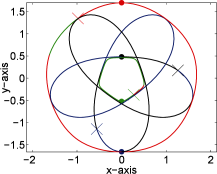
By taking θ=π5 in (1.1), a sample picture of the minimizer 𝒫0(t∈[0,1]) and its periodic extension is given in Figure 1.
In order to find local action minimizers connecting Qstart and Qend in (1.1), we define several closed subsets in ℝ6 and minimize 𝒜 over a→ in these subsets. So 24 subsets are defined as follows. We assume a2≥b2 and c2≥0 in (1.1), which is equivalent to fix a partial order of the bodies on the configuration Qend. For the collinear configuration Qstart, it has 24 different orders. Hence, 24 different subsets Γi(i=1,2…,24) can be defined by setting a2≥b2, c2≥0 in Qend and fixing the order of the four bodies in Qstart. For example, Γ1 is defined by
Γ
1
=
{
a
→
:
a
1
≤
b
1
≤
-
c
1
≤
c
1
-
a
1
-
b
1
,
a
2
≥
b
2
,
c
2
≥
0
}
,
which implies that the y-components of the four bodies at t=0 satisfy
q
1
y
(
0
)
≤
q
2
y
(
0
)
≤
q
3
y
(
0
)
≤
q
4
y
(
0
)
.
By Theorem 2.1, for each Γi(i=1,2,…,24), there exists an action minimizer 𝒫Γi∈H1([0,1],χ) connecting Qstart and Qend in (1.1):
𝒜
(
𝒫
Γ
i
)
=
inf
{
a
→
∈
Γ
i
}
inf
{
q
(
t
)
∈
P
(
Q
start
,
Q
end
)
}
𝒜
.
It is clear that the 24 local action minimizers are all different. However, some of them may contain collisions on Qstart or Qend. Furthermore, different action minimizers can be extended to the same solution of the N-body problem. By applying the first variation formulas and analyzing the equivalence relation between action minimizers 𝒫Γi(i=1,2,…,24), we show the following:
Theorem 1.2.
Assume that θ∈(0,π2) and θπ is rational. If all the minimizers PΓi(i=1,2,…,24) are classical solutions of the N-body problem, then there are sixteen different periodic orbits connecting Qstart and Qend defined in (1.1).
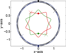
The proof of Theorem 1.2 can be found in Theorem 5.1. As a numerical evidence, we draw the motions of all the sixteen periodic orbits for θ=π5.
Structure of the paper.
The paper is organized as follows. Section 2 introduces a general coercivity result and shows the existence of 24 local action minimizers. Section 3 shows that the minimizer 𝒫0 is free of collision. In Section 4, we prove that 𝒫0 can be extended to a periodic or quasi-periodic orbit. In Section 5, we show that under appropriate assumptions, the 24 local action minimizers can be extended to sixteen nontrivial periodic orbits. Numerical evidences for θ=π5 are presented in the end.
2 Variational Settings and Coercivity
In this section, we introduce a general coercivity result (Theorem 2.1) of the Lagrangian action functional 𝒜 under structural prescribed boundary conditions in the N-body problem. Let χ={q∈ℝN×d:∑i=1Nmiqi=0}. We set
Q
start
=
[
q
1
(
a
1
,
…
,
a
k
)
⋮
q
N
(
a
1
,
…
,
a
k
)
]
,
Q
end
=
[
q
1
(
b
1
,
…
,
b
s
)
⋮
q
N
(
b
1
,
…
,
b
s
)
]
,
where qi∈ℝd(i=1,2,…,N,d=1,2,or3) are row vectors, and Qstart,Qend∈χ. Our variational argument is a two-step minimizing procedure. First, we consider a fixed-end boundary value problem, which is also known as the Bolza problem. For given values of a1,…,ak and b1,…,bs, the two matrices Qstart and Qend are fixed. There exists an action minimizer 𝒫, which satisfies
𝒜
(
𝒫
)
=
inf
{
q
(
t
)
∈
P
(
Q
start
,
Q
end
)
}
𝒜
=
inf
{
q
(
t
)
∈
P
(
Q
start
,
Q
end
)
}
∫
0
1
[
K
(
q
˙
(
t
)
)
+
U
(
q
(
t
)
)
]
𝑑
t
,
where P(Qstart,Qend) is defined as follows:
P
(
Q
start
,
Q
end
)
:=
{
q
(
t
)
∈
H
1
(
[
0
,
1
]
,
χ
)
:
q
(
0
)
=
Q
start
,
q
(
1
)
=
Q
end
}
.
If one wants 𝒫 to be a part of a periodic solution, the boundaries must be special and they should meet certain structural prescribed boundary conditions (SPBC). Hence, we introduce a second minimizing procedure. Instead of fixing the boundaries, we free several parameters on the boundaries q(0)=Qstart and q(1)=Qend. The Lagrangian action functional is then minimized over these parameters. The resulting minimizing path may be extended to a periodic or quasi-periodic solution. There are mainly three challenges to show the existence of such classical solutions. The first one is the coercivity of the Lagrangian action functional under the boundary constraints. The second one is to show the minimizer is collision-free on the boundaries. The third one is whether the minimizing path can be extended to a periodic or quasi-periodic solution. With an appropriate choice of SPBC, all the three challenges can be resolved. A general coercivity theorem [1] is introduced here to resolve the first challenge. For the reader’s convenience, a proof of the theorem is also given. The other two challenges will be resolved in Section 3 and Section 4.
Theorem 2.1.
Let
Q
start
=
[
q
1
(
a
1
,
…
,
a
k
)
⋮
q
N
(
a
1
,
…
,
a
k
)
]
,
Q
end
=
[
q
1
(
b
1
,
…
,
b
s
)
⋮
q
N
(
b
1
,
…
,
b
s
)
]
,
where Qstart,Qend∈χ, qi∈Rd, i=1,…,N, and a1,…,ak,b1,…,bs are independent variables. The matrix Qstart is linear with respect to ai(i=1,2,…,k) and Qend is linear with respect to bj(j=1,2,…,s). Let (a1,…,ak)∈S1,(b1,…,bs)∈S2, where S1⊂Rk and S2⊂Rs are closed subsets. Set S1∪S2=S. Assume that
{
Q
start
:
(
a
1
,
…
,
a
k
)
∈
ℝ
k
}
∩
{
Q
end
:
(
b
1
,
…
,
b
s
)
∈
ℝ
s
}
=
{
0
→
}
.
Then there exist a path sequence {Pnl} and a minimizer P0 in H1([0,1],χ) such that for each nl,
𝒜
(
𝒫
n
l
)
=
inf
{
q
(
0
)
=
Q
start
,
q
(
1
)
=
Q
end
,
q
(
t
)
∈
H
1
(
[
0
,
1
]
,
χ
)
,
a
i
=
a
i
n
l
,
b
j
=
b
j
n
l
(
i
=
1
,
…
,
k
,
j
=
1
,
…
,
s
)
}
𝒜
,
𝒜
(
𝒫
0
)
=
inf
{
(
a
1
,
…
,
a
k
,
b
1
,
…
,
b
s
)
∈
𝒮
}
inf
{
q
(
0
)
=
Q
start
,
q
(
1
)
=
Q
end
,
q
(
t
)
∈
H
1
(
[
0
,
1
]
,
χ
)
}
𝒜
=
inf
{
q
(
0
)
=
Q
start
,
q
(
1
)
=
Q
end
,
q
(
t
)
∈
H
1
(
[
0
,
1
]
,
χ
)
,
a
i
=
a
i
0
,
b
j
=
b
j
0
(
i
=
1
,
…
,
k
,
j
=
1
,
…
,
s
)
}
𝒜
.
For t∈[0,1], Pnl(t) converges to P0(t) uniformly. In particular,
lim
n
l
→
∞
a
i
n
l
=
a
i
0
,
lim
n
l
→
∞
b
j
n
l
=
b
j
0
,
i
=
1
,
…
,
k
,
j
=
1
,
…
,
s
.
Proof.
Note that L=K+U≥0, hence there exists some M0≥0 such that
inf
{
(
a
1
,
…
,
a
k
,
b
1
,
…
,
b
s
)
∈
𝒮
}
inf
{
q
(
0
)
=
Q
start
,
q
(
1
)
=
Q
end
,
q
(
t
)
∈
H
1
(
[
0
,
1
]
,
χ
)
}
𝒜
=
M
0
.
The proof follows by the Arzelà–Ascoli theorem. Basically, we can find a sequence 𝒫n, such that the action of the sequence 𝒜(𝒫n) approaches M0. Then we show the uniform boundedness and equicontinuity of the sequence. Hence, by the Arzelà–Ascoli theorem, there is a subsequence 𝒫nl which converges uniformly to a minimizer 𝒫0. Note that there exist sequences ain and bjn such that the minimum action value M0 can be reached by a path sequence 𝒫n∈H1([0,1],χ), which satisfies
𝒜
(
𝒫
n
)
=
inf
{
q
(
0
)
=
Q
start
,
q
(
1
)
=
Q
end
,
q
(
t
)
∈
H
1
(
[
0
,
1
]
,
χ
)
,
a
i
=
a
i
n
,
b
j
=
b
j
n
(
i
=
1
,
…
,
k
,
j
=
1
,
…
,
s
)
}
𝒜
,
and 𝒜(𝒫n)∈[M0,M0+12n]. It is clear that 𝒜(𝒫n)∈[M0,M0+1] for all n∈ℕ.
Next, we show the path sequence {𝒫n} is uniformly bounded. Let q(n)(t) be the position matrix path for {𝒫n}. We rewrite Qstart and Qend as (dN×1)-vectors:
Q
start
~
=
[
q
1
T
(
a
1
,
…
,
a
k
)
⋮
q
N
T
(
a
1
,
…
,
a
k
)
]
,
Q
end
~
=
[
q
1
T
(
b
1
,
…
,
b
s
)
⋮
q
N
T
(
b
1
,
…
,
b
s
)
]
.
Similarly, we can rewrite q(n)(t) as a (dN×1)-vector path q~(n)(t). By assumption, the two linear spaces satisfy
{
Q
start
:
(
a
1
,
…
,
a
k
)
∈
ℝ
k
}
∩
{
Q
end
:
(
b
1
,
…
,
b
s
)
∈
ℝ
s
}
=
{
0
→
}
.
Hence, Uk≡{Qstart~:(a1,…,ak)∈ℝk} is a k-dimensional linear space, Vs≡{Qend~:(b1,…,bs)∈ℝs} is a s-dimensional linear space, and Uk∩Vs={0}. Let {u1,…,uk} be an orthonormal basis of Uk and let {v1,…,vs} be an orthonormal basis of Vs.
For any nonzero vectors u→∈Uk and v→∈Vs, there exist constants gi,hj(1≤i≤k, 1≤j≤s) such that
u
→
|
u
→
|
=
g
1
u
1
+
…
+
g
k
u
k
,
∑
i
=
1
k
g
i
2
=
1
,
and
v
→
|
v
→
|
=
h
1
v
1
+
…
+
h
s
v
s
,
∑
j
=
1
s
h
j
2
=
1
.
Note that gi and hj(1≤i≤k,1≤j≤s) satisfy ∑i=1kgi2=∑j=1shj2=1. So they are on a compact set. It follows that the inner product of u→|u→| and v→|v→|,
〈
u
→
|
u
→
|
,
v
→
|
v
→
|
〉
=
∑
1
≤
i
≤
k
,
1
≤
j
≤
s
g
i
h
j
〈
u
i
,
v
j
〉
=
cos
(
u
→
,
v
→
)
,
can reach its maximum K0. If K0=1, there exist two vectors
u
→
∈
U
k
=
{
Q
start
~
:
(
a
1
,
…
,
a
k
)
∈
ℝ
k
}
and
v
→
∈
V
s
=
{
Q
end
~
:
(
b
1
,
…
,
b
s
)
∈
ℝ
s
}
such that u→|u→|=v→|v→|∈Uk∩Vs. Contradiction! Hence,
(2.1)
cos
(
u
→
,
v
→
)
≤
K
0
<
1
for any nonzero vectors
u
→
∈
U
k
,
v
→
∈
V
s
.
On the other hand, 𝒜(𝒫n)≤M0+1. If 0≤t1<t2≤1, we have
m
j
|
q
j
(
n
)
(
t
2
)
-
q
j
(
n
)
(
t
1
)
|
2
2
d
(
t
2
-
t
1
)
≤
∫
t
1
t
2
m
j
|
q
˙
j
(
t
)
|
2
2
𝑑
t
≤
𝒜
(
𝒫
n
)
≤
M
0
+
1
.
This implies that for any 1≤j≤N and any t1, t2 satisfying 0≤t1<t2≤1,
(2.2)
|
q
j
(
n
)
(
t
2
)
-
q
j
(
n
)
(
t
1
)
|
≤
2
d
(
t
2
-
t
1
)
(
M
0
+
1
)
m
j
.
Let m*=min{m1,m2,…,mN}. Then for all 1≤j≤N,
|
q
j
(
n
)
(
t
2
)
-
q
j
(
n
)
(
t
1
)
|
≤
2
d
(
M
0
+
1
)
m
*
.
In each 𝒫n, its element
q
(
n
)
(
t
)
=
[
q
1
(
n
)
⋮
q
N
(
n
)
]
can be rewritten as
q
~
(
n
)
(
t
)
=
[
(
q
1
(
n
)
)
T
⋮
(
q
N
(
n
)
)
T
]
.
Then for any t∈[0,1],
(2.3)
|
q
~
(
n
)
(
0
)
-
q
~
(
n
)
(
t
)
|
≤
N
2
d
(
M
0
+
1
)
m
*
.
Note that by (2.1), the angle between any two nonzero vectors
q
~
(
n
)
(
0
)
∈
{
Q
start
~
:
(
a
1
,
…
,
a
k
)
∈
𝒮
1
}
,
q
~
(
n
)
(
1
)
∈
{
Q
end
~
:
(
b
1
,
…
,
b
s
)
∈
𝒮
2
}
satisfies
〈
q
~
(
n
)
(
0
)
|
q
~
(
n
)
(
0
)
|
,
q
~
(
n
)
(
1
)
|
q
~
(
n
)
(
1
)
|
〉
=
cos
(
q
~
(
n
)
(
0
)
,
q
~
(
n
)
(
1
)
)
≤
K
0
<
1
.
It follows that
2
d
N
2
(
M
0
+
1
)
m
*
≥
|
q
~
(
n
)
(
0
)
-
q
~
(
n
)
(
1
)
|
2
=
|
q
~
(
n
)
(
0
)
|
2
+
|
q
~
(
n
)
(
1
)
|
2
-
2
|
q
~
(
n
)
(
0
)
|
|
q
~
(
n
)
(
1
)
|
cos
(
q
~
(
n
)
(
0
)
,
q
~
(
n
)
(
1
)
)
≥
|
q
~
(
n
)
(
0
)
|
2
+
|
q
~
(
n
)
(
1
)
|
2
-
2
K
0
|
q
~
(
n
)
(
0
)
|
|
q
~
(
n
)
(
1
)
|
=
[
K
0
|
q
~
(
n
)
(
0
)
|
-
|
q
~
(
n
)
(
1
)
|
]
2
+
(
1
-
K
0
2
)
|
q
~
(
n
)
(
0
)
|
2
≥
(
1
-
K
0
2
)
|
q
~
(
n
)
(
0
)
|
2
.
Hence
(2.4)
|
q
~
(
n
)
(
0
)
|
≤
2
d
N
2
(
M
0
+
1
)
m
*
(
1
-
K
0
2
)
.
By inequalities (2.3) and (2.4), it follows that for any t∈[0,1],
|
q
~
(
n
)
(
t
)
|
≤
|
q
~
(
n
)
(
0
)
-
q
~
(
n
)
(
t
)
|
+
|
q
~
(
n
)
(
0
)
|
≤
N
2
d
(
M
0
+
1
)
m
*
+
N
2
d
(
M
0
+
1
)
m
*
(
1
-
K
0
2
)
,
which is a uniform bound for |q~(n)(t)|. Therefore, the path sequence 𝒫n=𝒫n(t) is uniformly bounded.
Next, we show the path sequence {𝒫n=𝒫n(t)} is equicontinuous. In fact, by inequality (2.2),
|
q
j
(
n
)
(
t
2
)
-
q
j
(
n
)
(
t
1
)
|
≤
2
d
(
M
0
+
1
)
m
*
|
t
2
-
t
1
|
1
2
.
Then for any ϵ>0, let δ=ϵ2m*2d(M0+1). Whenever |t2-t1|≤δ, the following inequality holds:
|
q
j
(
n
)
(
t
2
)
-
q
j
(
n
)
(
t
1
)
|
≤
2
d
(
M
0
+
1
)
m
*
|
t
2
-
t
1
|
1
2
=
ϵ
.
It implies that for each j=1,2,…,N, qj(n)(t) is equicontinuous. It follows that the path sequence 𝒫n is equicontinuous.
By the Arzelà–Ascoli theorem, there exists a subsequence {𝒫nl} which converges uniformly. The limit 𝒫0=𝒫0(t) is in H1([0,1],χ) and it satisfies
lim
n
l
→
∞
𝒫
n
l
(
t
)
=
𝒫
0
(
t
)
for all
t
∈
[
0
,
1
]
.
In particular,
lim
n
l
→
∞
𝒫
n
l
(
0
)
=
𝒫
0
(
0
)
,
lim
n
l
→
∞
𝒫
n
l
(
1
)
=
𝒫
0
(
1
)
.
It follows that
lim
n
l
→
∞
a
i
n
l
=
a
i
0
,
lim
n
l
→
∞
b
j
n
l
=
b
j
0
,
i
=
1
,
…
,
k
,
j
=
1
,
…
,
s
,
and 𝒫0 satisfies
𝒜
(
𝒫
0
)
=
inf
{
q
(
0
)
=
Q
start
,
q
(
1
)
=
Q
end
,
q
(
t
)
∈
H
1
(
[
0
,
1
]
,
χ
)
,
a
i
=
a
i
0
,
b
j
=
b
j
0
(
i
=
1
,
…
,
k
,
j
=
1
,
…
,
s
)
}
𝒜
.
The proof is complete. ∎
As an application of Theorem 2.1, we first check if the two configurations Qstart and Qend defined in (1.1) satisfy the assumptions in Theorem 2.1. Recall that
Q
start
=
[
0
a
1
0
b
1
0
-
c
1
0
c
1
-
a
1
-
b
1
]
,
Q
end
=
[
0
a
2
0
b
2
-
c
2
-
a
2
+
b
2
2
c
2
-
a
2
+
b
2
2
]
R
(
θ
)
,
where a→=(a1,b1,c1,a2,b2,c2)∈ℝ6, and
R
(
θ
)
=
[
cos
(
θ
)
sin
(
θ
)
-
sin
(
θ
)
cos
(
θ
)
]
.
For any given θ∈(0,π2), it is clear that
{
Q
start
:
a
→
∈
ℝ
6
}
∩
{
Q
end
:
a
→
∈
ℝ
6
}
=
{
0
→
}
.
By Theorem 2.1, there exists an action minimizer 𝒫0∈H1([0,1],χ) and a vector a→0 such that
𝒜
(
𝒫
0
)
=
inf
{
a
→
∈
ℝ
6
}
inf
{
q
(
t
)
∈
P
(
Q
start
,
Q
end
)
}
𝒜
=
inf
{
q
(
t
)
∈
P
(
Q
start
,
Q
end
)
,
a
→
=
a
→
0
}
𝒜
.
In order to find local action minimizers, one can fix the order of the four bodies on Qend. We assume a2≥b2 and c2≥0, which means that at t=1, on the configuration Qend⋅R(-θ), body 1 is above body 2 on the y-axis and body 3 is on the left of body 4. We can then set different orders of the four bodies at t=0. Basically, the four bodies have 24 different orders on the y-axis at t=0. For each given order of the four bodies at t=0, we can define a subset Γi(i=1,2,…,24) of a→. It follows that we can define 24 different subsets of a→. For example, we define Γ1 as follows:
Γ
1
=
{
a
→
:
a
1
≤
b
1
≤
-
c
1
≤
c
1
-
a
1
-
b
1
,
a
2
≥
b
2
,
c
2
≥
0
}
,
which implies that the y-components of the four bodies at t=0 satisfy
q
1
y
(
0
)
≤
q
2
y
(
0
)
≤
q
3
y
(
0
)
≤
q
4
y
(
0
)
.
The other 23 subsets Γi(i=2,3,…,24) can be defined similarly. By Theorem 2.1, it follows that for each Γi(1≤i≤24), there exists a minimizer 𝒫Γi∈H1([0,1],χ) such that
𝒜
(
𝒫
Γ
i
)
=
inf
{
a
→
∈
Γ
i
}
inf
{
q
(
t
)
∈
P
(
Q
start
,
Q
end
)
}
𝒜
.
Remark.
Note that the boundary points of each Γi(1≤i≤24) are collisions. The possible collisions in the minimizer 𝒫Γi could be eliminated by using the level estimate method in [4, 5] or local deformation arguments in [16, 15] .
3 Exclusion of Collisions in 𝒫0
In this section, we prove the following:
Theorem 3.1.
The minimizing path P0 has no collision.
Note that the minimizing path 𝒫0 is defined for t∈[0,1]. By the celebrated results of Marchal [12] and Chenciner [7], 𝒫0 has no collision in (0,1). So we only need to exclude the possible collisions on boundaries q(0)=Qstart and q(1)=Qend. To exclude possible collision singularities of Qstart and Qend in the minimizer 𝒫0, we introduce the following theorem [1]:
Theorem 3.2 ([1, Theorem 4.3]).
Let S=Rk+s. If the intersection of the two configuration subsets is at origin, i.e.
{
Q
start
:
(
a
1
,
…
,
a
k
)
∈
ℝ
k
}
∩
{
Q
end
:
(
b
1
,
…
,
b
s
)
∈
ℝ
s
}
=
{
0
→
}
,
the action minimizer P0∈H1([0,1],χ) in Theorem 2.1 has no binary collision.
As an application, in our case a→=(a1,b1,c1,a2,b2,c2)∈ℝ6, it follows that there is no binary collision in 𝒫0.
Note that Qstart is a collinear configuration. We can then apply Chen’s result [3, 6] on collinear configurations to exclude possible collisions on Qstart:
Theorem 3.3 ([3, Theorem 2.1]).
In the minimizer P0, the collinear configuration Qstart has no collision singularity.
Furthermore, it is known that the bodies involved in a partial collision or total collision will approach a set of central configurations. More information can be known if the solution under concern is an action minimizer:
Lemma 3.1 ([14, Theorem 4.1.18] or [7, Section 3.2.1]).
If a minimizer q of the fixed-ends problem on time interval [τ1,τ2] has an isolated collision of k≤N bodies, then there is a parabolic homothetic collision-ejection solution q^ of the k-body problem which is also a minimizer of the fixed-ends problem on [τ1,τ2].
Lemma 3.2 ([3, Proposition 5] or [9, Section 7]).
Let X be a proper linear subspace of Rd. Suppose that a local minimizer x of At0,t1 on Bt0,t1(x(t0),X):={x∈H1([t0,t1],(Rd)N):x(t0) is fixed, xi(t1)∈X,i=1,2,…,N} has an isolated collision of k≤N bodies at t=t1. Then there is a homothetic parabolic solution y¯ of the k-body problem with y¯(t1)=0 such that y¯ is a minimizer of Aτ,t1* on Bτ,t1(y¯(τ),X) for any τ<t1. Here Aτ,t1* denotes the action of this k-body subsystem.
By Theorem 3.3, we are left to exclude possible collisions on Qend. The matrix form of Qend in (1.1) implies that Qend can be a double isosceles, a kite or a diamond. Hence it may have binary collisions, triple collisions and total collision. By Theorem 3.2, there is no binary collision on Qend. Hence, we need to exclude possible triple collisions and total collision on Qend of 𝒫0. We will use the level estimate method [4, 5] to exclude the total collision first.
Lemma 3.3.
In the minimizer P0, there is no total collision at t=1.
Proof.
We assume that at t=1, Qend experiences a total collision. Note that q∈χ. By Chen’s binary decomposition method [2, 5], the action can be written into the following form:
𝒜
=
∫
0
1
∑
i
=
1
4
1
2
|
q
˙
i
|
2
+
∑
1
≤
i
<
j
≤
4
1
|
q
i
-
q
j
|
d
t
=
1
4
∑
1
≤
i
<
j
≤
4
∫
0
1
1
2
|
q
˙
i
-
q
˙
j
|
2
+
4
|
q
i
-
q
j
|
d
t
.
By the estimates in [2, 5], if qi and qj(1≤i<j≤4) has a collision when t∈[0,1], the following inequality holds:
∫
0
1
1
2
|
q
˙
i
-
q
˙
j
|
2
+
4
|
q
i
-
q
j
|
d
t
≥
3
2
(
16
π
2
)
1
3
.
It follows that the action 𝒜totalcollision of a total collision path satisfies
𝒜
total
collision
≥
6
4
×
3
2
(
16
π
2
)
1
3
≥
12.16
.
For any given θ∈(0,π2), note that at t=1, the double isosceles configuration can be degenerated to a diamond configuration. A testing path can be defined as follows:
q
¯
1
=
2
e
(
θ
t
+
π
2
)
i
,
q
¯
2
=
-
q
¯
1
,
q
¯
3
=
e
[
(
θ
-
π
2
)
t
+
π
2
]
i
,
q
¯
4
=
-
q
¯
3
.
The action 𝒜¯ of this testing path is
𝒜
¯
=
∫
0
1
[
2
θ
2
+
(
π
2
-
θ
)
2
+
1
2
2
+
1
2
]
𝑑
t
+
∫
0
1
2
|
2
e
(
θ
t
+
π
2
)
i
+
e
[
(
θ
-
π
2
)
t
+
π
2
]
i
|
+
2
|
2
e
(
θ
t
+
π
2
)
i
-
e
[
(
θ
-
π
2
)
t
+
π
2
]
i
|
d
t
=
2
θ
2
+
(
π
2
-
θ
)
2
+
1
2
2
+
1
2
+
∫
0
1
2
3
+
2
2
cos
(
t
π
2
)
+
2
3
-
2
2
cos
(
t
π
2
)
d
t
≤
2
θ
2
+
(
π
2
-
θ
)
2
+
1
2
2
+
1
2
+
3.3386
.
Note that θ∈(0,π2), it follows that
𝒜
¯
≤
2
θ
2
+
(
π
2
-
θ
)
2
+
1
2
2
+
1
2
+
3.3386
<
π
2
2
+
1
2
2
+
1
2
+
3.3386
<
9.13
<
12.16
.
Therefore, there is no total collision at t=1 in the minimizer 𝒫0. The proof is complete. ∎
To exclude the possible triple collisions on Qend of the minimizer 𝒫0, we will apply the blow-up results in Lemma 3.1 and Lemma 3.2. Possible central configurations are discussed case by case so that we can lower the action by perturbation in each case. A local deformation argument is introduced in Lemma 3.4.
Lemma 3.4.
The minimizer P0 has no triple collision at t=1.
Proof.
The possible triple collisions in Qend could be a collision involving bodies 1, 3 and 4, or a collision involving bodies 2, 3 and 4. Note that in either case, the three bodies form an isosceles triangle configuration. Without loss of generality, we assume that the collision bodies are {1,3,4} and q2 is away from them on Qend. Note that θ∈(0,π2) is always fixed. For simplicity, we may shift the collision time from t=1 to t=0 and assume Qend to be
(3.1)
[
0
a
2
0
b
2
-
c
2
-
a
2
+
b
2
2
c
2
-
a
2
+
b
2
2
]
.
In the above configuration (3.1), the triple collision among bodies 1, 3 and 4 happens at t=0 when c2=0 and a2=-a2+b22≠b2.
By the analysis of the blow-up in Lemma 3.1 and Lemma 3.2, there exists a parabolic homothetic solution qi(t)=ait23(i=1,3,4), which is also a minimizer of the three-body problem on [0,τ] for any τ>0. For convenience, we denote the minimizer by q=(q1,q3,q4). Furthermore, (a1,a3,a4) forms a central configuration, and the three vectors a1, a3 and a4 satisfy the energy constraint
∑
i
=
1
,
3
,
4
1
2
|
2
3
a
i
|
2
-
∑
i
<
j
,
i
,
j
∈
{
1
,
3
,
4
}
1
|
a
i
-
a
j
|
=
0
.
Note that by the formula of Qend in (3.1), q1, q3 and q4 always form an isosceles triangle at t=0. To exclude the triple collision of q1, q3 and q4 at t=0, we need to show that the action 𝒜* of the subsystem (q=(q1,q3,q4) with qi=ait23(i=1,3,4)) can be lowered by deforming this parabolic homothetic solution under the boundary constraint at t=0. In fact, under this boundary constraint, it is challenging to apply the averaging method [12, 7, 9]. For this reason, the analysis of local deformation is done case by case for every possible central configuration.
Fix ϵ>0. When the central configuration of (q1,q3,q4) is an equilateral triangle, we use complex notations for simplicity. In fact, one can assume that a1=γeiθ0 with θ0∈[0,π] and γ=(332)13. The case when θ0∈[π,2π) can be handled similarly. Since there is no constraint on the order of body 3 and body 4 on the horizontal line, we can further assume that a3=a1e23πi,a4=a3e23πi. Now consider
q
~
1
=
r
(
t
)
e
i
θ
(
t
)
,
q
~
3
=
q
~
1
e
2
3
π
i
,
q
~
4
=
q
~
3
e
2
3
π
i
,
where
r
(
t
)
=
{
γ
(
ϵ
N
)
2
3
,
0
≤
t
≤
ϵ
N
,
γ
t
2
3
,
ϵ
N
≤
t
≤
ϵ
,
and θ(t)=(θ0-π2)tϵ+π2. At t=0, q~1(0)=r(0)eiθ(0), q~3(0)=q~1(0)e23πi and q~4(0)=q~3(0)e23πi, which satisfies the configuration Qend in (3.1). At t=ϵ, q~i(ϵ)=qi(ϵ)(i=1,3,4). Let 𝒜* be the action of the parabolic homothetic ejection solution qi(t)=ait23(i=1,2,4). Let 𝒜~* be the action of the perturbed path q~=(q~1,q~3,q~4). It follows that
𝒜
~
*
-
𝒜
*
=
(
(
9
γ
2
14
+
6
γ
2
7
N
7
3
)
(
θ
0
-
π
2
)
2
-
2
γ
2
+
2
3
γ
N
1
3
)
ϵ
1
3
.
By taking N=5, we have 𝒜~*-𝒜*<0 for every θ0∈[0,π].
When the central configuration of (q1,q3,q4) is an Euler collinear configuration, there must be one body staying at the origin. We discuss it in several cases. If a1=(0,0), a3=(ξ3,η3) and a4=-a3, then we define a perturbed path as follows:
q
~
1
=
q
1
,
q
~
3
=
(
ξ
3
ϵ
2
3
,
η
3
t
2
3
)
,
q
~
4
=
-
(
ξ
3
ϵ
2
3
,
η
3
t
2
3
)
,
where q~1(0)=(0,0), q~3(0)=(ξ3ϵ23,0) and q~4(0)=-(ξ3ϵ23,0) and at t=ϵ, q~i(ϵ)=qi(ϵ)(i=1,3,4). It is clear that 𝒜~*<𝒜* in this case.
If a1≠(0,0), then one of the other two bodies must stay at the origin. Without loss of generality, we can assume a3=(0,0). Let a1=(ξ1,η1). If η1≠0, we define
q
~
1
=
(
ξ
1
t
2
3
,
η
1
ϵ
2
3
)
,
q
~
3
=
(
0
,
-
η
1
2
(
ϵ
2
3
-
t
2
3
)
)
,
q
~
4
=
(
-
ξ
1
t
2
3
,
-
η
1
2
(
ϵ
2
3
+
t
2
3
)
)
,
where q~1(0)=(0,η1ϵ23), q~3(0)=(0,-η12ϵ23) and q~4(0)=(0,-η12ϵ23) and at t=ϵ, q~i(ϵ)=qi(ϵ),(i=1,3,4). It follows that the kinetic energy is decreased, and
|
q
~
3
-
q
~
4
|
=
|
q
3
-
q
4
|
,
|
q
~
1
-
q
~
4
|
≥
|
q
1
-
q
4
|
.
For t∈[0,ϵ],
|
q
~
1
-
q
~
3
|
=
(
ξ
1
2
+
η
1
2
4
)
t
4
3
-
3
2
η
1
2
ϵ
2
3
t
2
3
+
9
4
η
1
2
ϵ
4
3
≥
(
ξ
1
2
+
η
1
2
4
)
t
4
3
+
3
4
η
1
2
ϵ
4
3
.
It implies that
∫
0
ϵ
d
t
|
q
~
1
-
q
~
3
|
<
∫
0
ϵ
d
t
|
q
1
-
q
3
|
and
∫
0
ϵ
d
t
|
q
~
1
-
q
~
4
|
<
∫
0
ϵ
d
t
|
q
1
-
q
4
|
.
Hence, 𝒜~*<𝒜*.
If η1=0 and ξ1≠0, then
q
1
=
(
ξ
1
t
2
3
,
0
)
,
q
3
=
(
0
,
0
)
,
q
4
=
(
-
ξ
1
t
2
3
,
0
)
.
In this case we define
q
~
1
=
(
ξ
1
t
2
3
,
2
δ
(
1
-
t
2
3
ϵ
2
3
)
)
,
q
~
3
=
(
0
,
-
δ
(
1
-
t
2
3
ϵ
2
3
)
)
,
q
~
4
=
(
-
ξ
1
t
2
3
,
-
δ
(
1
-
t
2
3
ϵ
2
3
)
)
,
where q~1(0)=(0,2δ), q~3(0)=(0,-δ) and q~4(0)=(0,-δ) and at t=ϵ, q~i(ϵ)=qi(ϵ)(i=1,3,4). We set
δ
=
ϵ
2
3
N
.
Let K* be the kinetic energy of the subsystem q=(q1,q3,q4). Let K~* be the kinetic energy of the perturbed path q~=(q~1,q~3,q~4). It follows that
△
K
*
=
∫
0
ϵ
(
K
~
*
-
K
*
)
𝑑
t
=
4
N
ϵ
1
3
.
A direct calculation implies that
|
q
~
1
-
q
~
3
|
≥
9
ξ
1
2
N
ξ
1
2
+
9
ϵ
2
3
,
|
q
~
1
-
q
~
4
|
≥
36
ξ
1
2
4
N
ξ
1
2
+
9
ϵ
2
3
,
|
q
~
3
-
q
~
4
|
=
|
ξ
1
|
t
2
3
.
It follows that
(3.2)
𝒜
~
*
-
𝒜
*
≤
[
4
N
+
(
9
ξ
1
2
N
ξ
1
2
+
9
)
-
1
2
+
(
36
ξ
1
2
4
N
ξ
1
2
+
9
)
-
1
2
-
9
2
|
ξ
1
|
]
ϵ
1
3
.
Note that in the Euler central configuration, ξ1=(458)13. By taking N=6 in (3.2), we have 𝒜~*-𝒜*<0.
Therefore, for all possible central configurations of q=(q1,q3,q4), there always exists some perturbed path q~, such that
𝒜
~
*
-
𝒜
*
<
0
.
Contradiction! It implies that there is no triple collision among q1, q3 and q4 in the minimizer 𝒫0. Similarly, we can show that there is no triple collision among q2, q3 and q4 in 𝒫0. The proof is complete. ∎
The proof of Theorem 3.1 follows by Theorem 3.2, Theorem 3.3, Lemma 3.3 and Lemma 3.4. Hence, the minimizer 𝒫0=𝒫0(t∈[0,1]) is a classical solution of the N-body problem. However, it is hard to eliminate possible collisions in each 𝒫Γi(i=1,2,…,24). We will check them numerically.
4 Extension of the Minimizer 𝒫0
By the previous section, we know that 𝒫0(t∈[0,1]) is a classical solution of the N-body problem. In this section, we show that the minimizer 𝒫0(t∈[0,1]) can be extended to a periodic or quasi-periodic orbit. First variation formulas are applied to the variables a1,b1,c1 in Qstart and a2,b2,c2 in Qend of the minimizer 𝒫0, which imply several identities of the velocities on both boundaries. An extension formula of 𝒫0(t∈[0,1]) can then be defined by (4.2) in Theorem 4.1.
Proposition 4.1.
In the minimizer P0, the velocities q˙i(t)(i=1,2,3,4) satisfy
q
˙
1
y
(
0
)
=
q
˙
2
y
(
0
)
=
q
˙
3
y
(
0
)
=
q
˙
4
y
(
0
)
=
0
,
and
q
˙
1
(
1
)
=
-
q
˙
1
(
1
)
B
R
(
2
θ
)
,
q
˙
3
(
1
)
=
-
q
˙
4
(
1
)
B
R
(
2
θ
)
,
q
˙
2
(
1
)
=
-
q
˙
2
(
1
)
B
R
(
2
θ
)
,
q
˙
4
(
1
)
=
-
q
˙
3
(
1
)
B
R
(
2
θ
)
,
where
B
=
[
-
1
0
0
1
]
𝑎𝑛𝑑
R
(
2
θ
)
=
[
cos
(
2
θ
)
sin
(
2
θ
)
-
sin
(
2
θ
)
cos
(
2
θ
)
]
.
Proof.
Note that there exists some a0→∈ℝ6 such that
𝒜
(
𝒫
0
)
=
inf
{
q
(
t
)
∈
P
(
Q
start
,
Q
end
)
,
a
→
=
a
→
0
}
𝒜
.
Let q=q(t) be the position matrix path of 𝒫0. Consider an admissible variation ξ(t)∈P(Qstart,Qend) satisfying ξ(0)∈{Qstart:(a1,…,ak)∈𝒮1} and ξ(1)∈{Qend:(b1,…,bs)∈𝒮2}; then the first variation δξ𝒜(q) satisfies
0
=
δ
ξ
𝒜
(
q
)
=
lim
τ
→
0
𝒜
(
q
+
τ
ξ
)
-
𝒜
(
q
)
τ
=
∫
0
1
1
2
∑
i
=
1
4
lim
τ
→
0
m
i
∥
q
˙
i
+
τ
ξ
˙
i
∥
2
-
∥
q
˙
i
∥
2
τ
+
lim
τ
→
0
U
(
q
+
τ
ξ
)
-
U
(
q
)
τ
d
t
=
∫
0
1
(
∑
i
=
1
4
m
i
〈
q
˙
i
,
ξ
˙
i
〉
+
∑
i
=
1
4
〈
∂
∂
q
i
U
(
q
(
t
)
)
,
ξ
i
〉
)
𝑑
t
=
∑
i
=
1
4
(
m
i
〈
q
˙
i
,
ξ
i
〉
|
t
=
0
t
=
1
+
∫
0
1
〈
-
m
i
q
¨
i
+
∂
∂
q
i
U
(
q
(
t
)
)
,
ξ
i
〉
𝑑
t
)
(4.1)
=
∑
i
=
1
4
m
i
〈
q
˙
i
,
ξ
i
〉
|
t
=
0
t
=
1
.
Note that m1=m2=m3=m4=1. Let ξ(t)∈P(Qstart,Qend) such that
ξ
(
0
)
=
[
0
1
0
0
0
0
0
-
1
]
and
ξ
(
1
)
=
0
.
By identity (4.1), it follows that
q
˙
1
y
(
0
)
-
q
˙
4
y
(
0
)
=
0
.
Similarly, by taking different values of ξ(0), we have
q
˙
2
y
(
0
)
-
q
˙
4
y
(
0
)
=
0
,
-
q
˙
3
y
(
0
)
+
q
˙
4
y
(
0
)
=
0
.
Note that
∑
i
=
1
4
q
˙
i
y
(
0
)
=
0
.
It follows that
q
˙
1
y
(
0
)
=
q
˙
2
y
(
0
)
=
q
˙
3
y
(
0
)
=
q
˙
4
y
(
0
)
=
0
.
Similar arguments on a2,b2,c2 imply that
q
˙
1
(
1
)
=
-
q
˙
1
(
1
)
B
R
(
2
θ
)
,
q
˙
3
(
1
)
=
-
q
˙
4
(
1
)
B
R
(
2
θ
)
,
q
˙
2
(
1
)
=
-
q
˙
2
(
1
)
B
R
(
2
θ
)
,
q
˙
4
(
1
)
=
-
q
˙
3
(
1
)
B
R
(
2
θ
)
,
where
B
=
[
-
1
0
0
1
]
and
R
(
2
θ
)
=
[
cos
(
2
θ
)
sin
(
2
θ
)
-
sin
(
2
θ
)
cos
(
2
θ
)
]
.
The proof is complete. ∎
The extension of the path 𝒫0(t∈[0,1]) then follows by Proposition 4.1 and the uniqueness of solutions of an ODE system.
Theorem 4.1.
Let θ∈(0,π2). If θπ is rational, the minimizer P0(t∈[0,1]) can be extended to a periodic orbit. Otherwise, P0(t∈[0,1]) can be extended to a quasi-periodic orbit.
Proof.
Let
q
(
t
)
=
[
q
1
(
t
)
q
2
(
t
)
q
3
(
t
)
q
4
(
t
)
]
,
t
∈
[
0
,
1
]
,
be the position matrix path of the minimizer 𝒫0(t∈[0,1]), where each qi(t)=(qix(t),qiy(t))(i=1,2,3,4) is a 2-dimensional row vector path. Its extension is defined as follows:
(4.2)
q
(
t
)
=
{
(
q
1
T
(
t
)
,
q
2
T
(
t
)
,
q
3
T
(
t
)
,
q
4
T
(
t
)
)
T
,
t
∈
[
0
,
1
]
,
(
q
1
T
(
2
-
t
)
,
q
2
T
(
2
-
t
)
,
q
4
T
(
2
-
t
)
,
q
3
T
(
2
-
t
)
)
T
B
R
(
2
θ
)
,
t
∈
[
1
,
2
]
,
(
q
1
T
(
t
-
2
)
,
q
2
T
(
t
-
2
)
,
q
4
T
(
t
-
2
)
,
q
3
T
(
t
-
2
)
)
T
R
(
2
θ
)
,
t
∈
[
2
,
4
]
,
q
(
t
-
4
k
)
R
(
4
k
θ
)
,
t
∈
[
4
k
,
4
k
+
4
]
,
where
B
=
[
-
1
0
0
1
]
and k∈ℤ. Recall that
Q
start
=
[
0
a
1
0
b
1
0
-
c
1
0
c
1
-
a
1
-
b
1
]
,
Q
end
=
[
0
a
2
0
b
2
-
c
2
-
a
2
+
b
2
2
c
2
-
a
2
+
b
2
2
]
R
(
θ
)
.
By Proposition 4.1, it follows that at t=1, q(t) is actually C1. Since q(t) satisfies the Newtonian equation, it follows that q(t) is smooth at t=1. And at t=2, the four bodies are on a line which is a counterclockwise 2θ rotation of the y-axis. Each velocity q˙i(i=1,2,3,4) at t=2 is perpendicular to the line of their configuration. Similarly, we can show that the orbit q(t) is smooth at t=2. Note that when t=4, the position matrix q and the velocity matrix q˙ satisfy
q
(
4
)
=
q
(
0
)
R
(
4
θ
)
,
q
˙
(
4
)
=
q
˙
(
0
)
R
(
4
θ
)
.
By the uniqueness of solutions of an ODE system, the extension of q(t)(t∈[0,4]) is
q
(
t
)
=
q
(
t
-
4
k
)
R
(
4
k
θ
)
,
t
∈
[
4
k
,
4
k
+
4
]
,
where k∈ℤ. Therefore, the definition of q(t) in (4.2) is smooth for all t. If θπ=k1l1 is rational (k1,l1 are integers), then the minimizer 𝒫0(t∈[0,1]) can be extended to a periodic orbit with a period T=4l1. If θπ is irrational, then the extension of 𝒫0(t∈[0,1]) in (4.2) is quasi-periodic. The proof is complete. ∎
Remark.
If the local action minimizers 𝒫Γi(t∈[0,1])(i=1,2,…,24) are collision-free, similar arguments can be applied to show that each 𝒫Γi(i=1,2,…,24) can be extended to a periodic or quasi-periodic orbit. And their extensions satisfy the same formula of q(t) in (4.2).
5 Equivalence of Action Minimizers
In the last section, we discuss the equivalent class of all the 24 local action minimizers 𝒫Γi(i=1,2,…,24). By assuming that θπ is rational and each minimizer 𝒫Γi(i=1,2,…,24) is a classical solution, we show that these 24 action minimizers can actually generate sixteen different periodic orbits.
Recall that each local action minimizer 𝒫Γi(i=1,2,…,24) satisfies
𝒜
(
𝒫
Γ
i
)
=
inf
{
a
→
∈
Γ
i
}
inf
{
q
(
t
)
∈
P
(
Q
start
,
Q
end
)
}
𝒜
,
where Γi is defined as follows. In every Γi(i=1,2,…,24), we assume that the variables on Qend always satisfy a2≥b2 and c2≥0. Then in the collinear configuration Qstart, the 24 different orders Δ=(α1,α2,α3,α4) of the four bodies at t=0 have a one-to-one correspondence to the 24 action minimizers 𝒫Γi(i=1,2,…,24). For example, we define Γ1 as
Γ
1
=
{
a
→
:
a
1
≤
b
1
≤
-
c
1
≤
-
a
1
-
b
1
+
c
1
,
a
2
≥
b
2
,
c
2
≥
0
}
,
which has the following order at t=0:
q
1
y
(
0
)
≤
q
2
y
(
0
)
≤
q
3
y
(
0
)
≤
q
4
y
(
0
)
.
We denote it by (1,2,3,4). That is, the minimizer 𝒫Γ1 corresponds to an order (1,2,3,4) in Qstart. The following result shows that some of the orders in Qstart correspond to the same solution of the four-body problem.
Lemma 5.1.
Given a2≥b2,c2≥0, the orders Δ and σ1σ2Δ in Qstart correspond to the same periodic solution, where
σ
1
=
(
12
)
(
34
)
,
σ
2
=
(
α
1
α
2
α
3
α
4
α
4
α
3
α
2
α
1
)
.
Proof.
Note that q(t) and -q(t) are considered as the same solution in the N-body problem. Assume that q(0) has an order Δ=(α1,α2,α3,α4) in Qstart; then -q(0) has an order
(
α
4
,
α
3
,
α
2
,
α
1
)
=
σ
2
Δ
,
where
σ
2
=
(
α
1
α
2
α
3
α
4
α
4
α
3
α
2
α
1
)
.
But the corresponding Qend in -q(t) has a2≤b2 and c2≤0. Let σ1=(12)(34). Then in the orbit corresponding to σ1σ2Δ, Qend satisfies a2≥b2 and c2≥0. It implies that Δ and σ1σ2Δ=σ2σ1Δ correspond to the same orbit. The proof is complete. ∎
Theorem 5.1.
Assume that θ∈(0,π2) and θπ is rational. If all the minimizers PΓi(i=1,2,…,24) are classical solutions of the N-body problem, then there are sixteen different periodic orbits connecting Qstart and Qend defined in (1.1).
Proof.
For convenience, we use Δα1α2α3α4 to represent the corresponding action minimizer. For example, 𝒫Γ1 corresponds to Δ1234. By Lemma 5.1, we know that the 24 action minimizers can be classified into the following sixteen sets:
{
Δ
1234
,
Δ
3412
}
,
{
Δ
1243
,
Δ
4312
}
,
{
Δ
1324
,
Δ
3142
}
,
{
Δ
1423
,
Δ
4132
}
,
{
Δ
2134
,
Δ
3421
}
,
{
Δ
2143
,
Δ
4321
}
,
{
Δ
2314
,
Δ
3241
}
,
{
Δ
2413
,
Δ
4231
}
,
{
Δ
1342
}
,
{
Δ
1432
}
,
{
Δ
2341
}
,
{
Δ
2431
}
,
{
Δ
3124
}
,
{
Δ
3214
}
,
{
Δ
4123
}
,
{
Δ
4213
}
.
Therefore, there are sixteen different periodic orbits connecting Qstart and Qend defined in (1.1). The proof is complete. ∎
In the end, numerical results are presented for some rotation angle θ. Note that by the definitions of Qstart and Qend in (1.1), it is easy to check that 𝒫Γi(i=1,2,…,24) cannot be a relative equilibrium in the four-body problem. In other words, these sixteen periodic orbits are nontrivial. Numerically, we set θ=π5 and calculate the sixteen action minimizers by Matlab. The motions of the sixteen periodic orbits can then be drawn as in Figure 2. It is worth mentioning that some of the orbits are very complicated. It will be interesting if one can analytically prove their existences. For other values of θ∈(0,π2), similar multiplicity results of periodic orbits are expected.
Figure 2
Sixteen different periodic orbits connecting Qstart and Qend in (1.1) with θ=π5.
 and
Tiancheng Ouyang
and
Tiancheng Ouyang