1 Introduction
The study of periodically perturbed homoclinic solutions originated from the work of Poincaré [14, 15, 16, 17], whose pioneer observation on the existence of homoclinic tangles induced by non-tangential intersections of the stable and the unstable manifold has been regarded as the starting point of the modern chaos theory. Poincaré discovered that, when a homoclinic solution of a saddle fixed point is periodically perturbed, the simple homoclinic loop in phase space would break into two intersecting curves. The two curves would then be forced to further intersect to form a web, the structure of which appeared to be incomprehensibly complicated.
From the time of Poincaré to the early 1960s, many, including Birkhoff [4], Cartwright and Littlewood [6], Levinson [12], Sitnikov [18], and Alekseev [1, 2, 3], had studied more systems of differential equations from various disciplines of applied science, and they confirmed the existence of homoclinic tangle in quite a few equations of historic and practical importance. Some also came to the conclusion that periodic solutions accumulate in homoclinic tangle. Birkhoff and Levinson even used symbolic sequences to code the solutions. Built on these studies, Smale proposed a rather straightforward dynamical structure that has been commonly referred to as Smale’s horseshoe in later times. He observed that a horseshoe map is embedded in all homoclinic tangles [19]. The Melnikov method was then introduced to apply Smale’s theory of horseshoes to periodically perturbed equations [13]. The combination of the theory of Smale’s horseshoe and the Melnikov method has become a main venue [8], through which the modern chaos theory has been applied to the study of numerous problems in applied sciences.
The setting for the Melnikov method is as follows: We start with a 2D autonomous equation
(1.1)
d
x
d
t
=
F
(
x
,
y
)
,
d
y
d
t
=
G
(
x
,
y
)
.
Assume that (1.1) has a saddle fixed point p0=(x0,y0) with a homoclinic solution, which we denote as
ℓ
=
{
(
a
(
t
)
,
b
(
t
)
)
:
t
∈
(
-
∞
,
+
∞
)
}
.
Let Dℓ be a small neighborhood of the homoclinic loop ℓ∪(x0,y0). We assume F(x,y), G(x,y) are real analytic on Dℓ. To equation (1.1) we add a time-periodic perturbation to obtain
(1.2)
d
x
d
t
=
F
(
x
,
y
)
+
ε
P
(
x
,
y
,
t
,
ε
)
,
d
y
d
t
=
G
(
x
,
y
)
+
ε
Q
(
x
,
y
,
t
,
ε
)
,
where ε∈Iε0:=(-ε0,ε0) is a small parameter, and P(x,y,t,ε) and Q(x,y,t,ε) are real analytic on
(
x
,
y
,
t
,
ε
)
∈
D
ℓ
×
(
-
∞
,
+
∞
)
×
I
ε
0
.
We assume P, Q are periodic in t. That is to say that there exists a constant T>0 so that
P
(
x
,
y
,
t
,
ε
)
=
P
(
x
,
y
,
t
+
T
,
ε
)
,
Q
(
x
,
y
,
t
)
=
Q
(
x
,
y
,
t
+
T
,
ε
)
.
Without loss of generality, we let P(x0,y0,t,ε)=Q(x0,y0,t,ε)=0 for all t and ε to fix the saddle point at (x0,y0).
We treat ε as a fixed parameter. Let 𝐧=(b˙(0),-a˙(0)) be perpendicular to ℓ at ℓ(0)=(a(0),b(0)), and let
Σ
=
{
(
a
(
0
)
,
b
(
0
)
)
+
z
⋅
𝐧
:
|
z
|
<
K
-
1
}
.
The set Σ is a line segment centered at ℓ(0). For a given t0, we let (x+(t,t0),y+(t,t0)) be a solution of (1.2) so that
(x+(t,t0),y+(t,t0))∈Dℓ for all t∈[t0,+∞),
p+:=(x+(t0,t0),y+(t0,t0))∈Σ.
Then we call (x+(t,t0),y+(t,t0)) a primary stable solution. Similarly, we let (x-(t,t0),y-(t,t0)) be a solution so that
(x-(t,t0),y-(t,t0))∈Dℓ for all t∈(-∞,t0],
p-:=(x-(t0,t0),y-(t0,t0))∈Σ.
Then we call (x-(t,t0),y-(t,t0)) a primary unstable solution. Both the primary stable and the primary unstable solution are uniquely determined for a given t0. Let D(ε,t0) be such that
D
(
ε
,
t
0
)
⋅
𝐧
=
p
+
-
p
-
=
(
x
+
(
t
0
,
t
0
)
,
y
+
(
t
0
,
t
0
)
)
-
(
x
-
(
t
0
,
t
0
)
,
y
-
(
t
0
,
t
0
)
)
.
See Figure 1. We name D(ε,t0) the splitting distance, which is a function of ε and t0.
We expand D(ε,t0) as a power series of ε in the form of
D
(
ε
,
t
0
)
=
M
0
(
t
0
)
ε
+
M
1
(
t
0
)
ε
2
+
M
2
(
t
0
)
ε
3
+
⋯
+
M
k
(
t
0
)
ε
k
+
1
+
⋯
.
In [13], Melnikov introduced an inductive scheme to compute M0,M1,…,Mn,…. For M0(t0), he derived an integral formula, in which the integrand is obtained as an explicit function of ℓ(t) through F, G, P, Q. Melnikov used the equations of first variations around the homoclinic solution ℓ(t-t0) to calculate the primary stable and unstable solution up to the precision of order ε. He projected the solutions of the equations of the first variations into the direction that is perpendicular to ℓ(t-t0), and made the observation that the equation for the projected normal component is self-sustained. Separating this equation out from the rest, he reduced the task of computing M0(t0) to that of solving a first-order linear non-autonomous equation. The self-reliance of the normal component to ℓ(t-t0) appeared to be the key, from which an explicit integral formula for M0(t0) followed.
Next we turn to the problem of computing higher-order coefficients Mk(t0) for k=1,2,…. Suppose (x(t,t0,ε),y(t,t0,ε)) to be the stable solutions. We expand this solution into a power series of ε as
x
(
t
,
t
0
,
ε
)
=
x
0
(
t
,
t
0
)
+
ε
x
1
(
t
,
t
0
)
+
⋯
+
ε
n
x
n
(
t
,
t
0
)
+
⋯
,
y
(
t
,
t
0
,
ε
)
=
y
0
(
t
,
t
0
)
+
ε
y
1
(
t
,
t
0
)
+
⋯
+
ε
n
y
n
(
t
,
t
0
)
+
⋯
.
We denote the truncations to order εn of this solution as
X
(
n
)
(
t
,
t
0
,
ε
)
=
x
0
(
t
,
t
0
)
+
ε
x
1
(
t
,
t
0
)
+
⋯
+
ε
n
x
n
(
t
,
t
0
)
,
Y
(
n
)
(
t
,
t
0
,
ε
)
=
y
0
(
t
,
t
0
)
+
ε
y
1
(
t
,
t
0
)
+
⋯
+
ε
n
y
n
(
t
,
t
0
)
.
Melnikov introduced the following inductive process to compute (xn(t0,t0),yn(t0,t0)):
Inductive Assumption: We know the explicit formula for X(n)(t,t0,ε), Y(n)(t,t0,ε) for a given integer n≥0.
We do the following to compute X(n+1)(t,t0,ε), Y(n+1)(t,t0,ε):
Deriving the Equations of Variations: First we derive an equation for (xn+1(t,t0),yn+1(t,t0)) by using X(n)(t,t0,ε), Y(n)(t,t0,ε). This is a set of non-autonomous equations of two variables.
Solving the Equations of Variations: We solve the variational equation to obtain a general solution formula. Here the self-sustained nature of the normal component is again the key.
Determining the Initial Condition for Stable Solutions: Using the general solution obtained in (ii), we can determine the initial condition (xn+1(t0,t0),yn+1(t0,t0)) for stable solutions.
Continuing the Induction: To continue the induction, we substitute the result of (iii) back into (ii) to obtain (xn+1(t,t0),yn+1(t,t0)).
In this paper, however, we pursue an entirely different route. Our method to compute the stable solutions (x(t,t0,ε),y(t,t0,ε)) is as follows:
Working with the original perturbed equation, we can derive an integral formula for the initial condition of the stable solutions in the form of
x
(
t
0
,
t
0
,
ε
)
=
F
(
a
(
t
)
,
b
(
t
)
,
t
,
x
(
t
,
t
0
,
ε
)
,
y
(
t
,
t
0
,
ε
)
,
ε
)
,
y
(
t
0
,
t
0
,
ε
)
=
G
(
a
(
t
)
,
b
(
t
)
,
t
,
x
(
t
,
t
0
,
ε
)
,
y
(
t
,
t
0
,
ε
)
,
ε
)
(see (4.6)). That is to say that, instead of explicitly solving for xn(t0,t0), yn(t0,t0) step by step in an inductive process relying on equations of variations and the solutions of lower order, as proposed by Melnikov, we write the initial condition for stable solutions up to infinite precision in terms of the integrals of the stable solution x(t,t0,ε), y(t,t0,ε) in a single step.
We then derive two integral equations for x(t,t0,ε), y(t,t0,ε) (see (4.6) and (4.7)) by using (i).
We now write x(t,t0,ε), y(t,t0,ε) as a power series in ε, substituting it into (4.6) and (4.7) to recursively solve for x1(t,t0),y1(t,t0),x2(t,t0),y2(t,t0),….
The main difference of our method and Melnikov’s method is as follows: In Melnikov’s method, the problem of solving x(t,t0,ε), y(t,t0,ε) is mixed up with the problem of solving the initial condition for stable solutions x(t0,t0,ε), y(t0,t0,ε) in an inductive process that involves solving equations of variations in every step of the way. In our method, these two problems are completely separated. There is no induction nor equations of variations involved in deriving item (i). All it takes is to re-write the unperturbed equation in a set of new coordinates, that is, with clear geometric interpretation. Item (ii) follows trivially from (i). By the time we reach (iii), the problem of determining the initial conditions for stable solutions is completely out of the way.
The results of this paper are briefly summarized as follows:
We prove that, for all k, Mk(t0) is a sum of certain multiple integrals, the integrands of which are explicit functions of ℓ(t) through F, G, P, Q. We name these integrals as high-order Melnikov integrals.
In particular, we derive formulas for M0(t0) and M1(t0) in integral form, in which all integrands are obtained as explicit functions of ℓ(t) through F, G, P, Q.
We use the acquired formulas for M0(t0) and M1(t0) to study a concrete equation. In particular, the explicit formula of M1(t0) is used to prove the existence of transversal homoclinic intersection in the case of M0(t0)≡0.
To the best of our knowledge, this is the first time M1(t0) is acquired in its entirety for time-periodic equations as explicit integrals in ℓ(t). Our theory on higher-order Melnikov integrals for Mk(t0) is also new.
We note that there has also been a body of previous work on the high-order Melnikov method on equations with autonomous perturbations. These studies cover a variety of subjects including the issues of bifurcations of homoclinic solutions in autonomous equations [21, 22, 23], and the existence of periodic solutions in polynomial systems in conjunction with the study of Hilbert’s sixteenth problem [5, 7, 9, 10, 11, 20]. These studies, however, are not related to the new method introduced in this paper.
We would also like to make the following apparent: it is one thing to obtain Mk(t0) as explicit integrals in ℓ(t), but it is an entirely different thing to analytically evaluate these integrals. While we can achieve the former for a rather generic setting, we have not yet been able to come up with a nontrivial example for which M1(t0) is evaluated through the integrals derived in this paper in close form. For the example presented in this paper, these integrals are evaluated numerically by using Simpson’s rule.
2 Statement of Results
Without loss of generality, we let (x0,y0)=(0,0) be the saddle fix point to write the unperturbed equation as
(2.1)
d
x
d
t
=
-
α
x
+
f
(
x
,
y
)
,
d
y
d
t
=
β
y
+
g
(
x
,
y
)
.
We study the perturbed equation in the form of
(2.2)
d
x
d
t
=
-
α
x
+
f
(
x
,
y
)
+
ε
sin
t
⋅
P
(
x
,
y
)
,
d
y
d
t
=
β
y
+
g
(
x
,
y
)
+
ε
sin
t
⋅
Q
(
x
,
y
)
,
where ε∈Iε0:=(-ε0,ε0) is a small parameter. Here we chose to work with perturbations in the form of εsint⋅P(x,y) and εsint⋅Q(x,y) for the sake of a clean-cut presentation. Our method works just the same for equation (1.2), but the presentation would be a little messier: we would need to first expand P(t,x,y,ε), Q(t,x,y,ε) as power series in ε and treat each of the coefficients of this expansion as a function of t, x, y that is periodic in t. The generic structure of the high-order Melnikov integrals would remain the same but the kernel functions would be t-periodic. In particular, there will be additional integrals for M1 coming from the first-order terms of P(t,x,y,ε) and Q(t,x,y,ε). The same computations, however, apply without glitch.
We assume the following for equations (2.1) and (2.2):
Homoclinic Solution: The unperturbed equation (2.1) has a homoclinic solution ℓ(t)=(a(t),b(t)) satisfying limt→±∞ℓ(t)=(0,0).
On Unperturbed Equations: Let Dℓ be a small neighborhood of the homoclinic loop
{
ℓ
(
t
)
:
t
∈
(
-
∞
,
+
∞
)
}
∪
(
0
,
0
)
.
The functions f(x,y), g(x,y) are real analytic on Dℓ and they are of order two and higher at (0,0). We also have α,β>0.
On Perturbation Function:P(x,y),Q(x,y) are real analytic on Dℓ, and they are terms of second order and higher at (x,y)=(0,0).
2.1 High-Order Melnikov Method
Proposition 2.1.
There exists an ε0>0 sufficiently small so that the splitting distance D(ε,t0) can be written as a uniformly convergent power series of ε on Iε0 in the form of
D
(
ε
,
t
0
)
=
M
0
(
t
0
)
ε
+
M
1
(
t
0
)
ε
2
+
M
2
(
t
0
)
ε
3
+
⋯
+
M
k
(
t
0
)
ε
k
+
1
+
⋯
.
In addition, all Mk(t0), k≥0, are analytic functions of t0 for all t0.
We now present explicit integral formulas for M0(t0) and M1(t0). Let ℓ(t)=(a(t),b(t)) be the homoclinic solution of the unperturbed equation. We denote a=a(t), b=b(t), a˙=ddta(t), b˙=ddtb(t), and so on.
(A) Integral for M0(t0): We have
(2.3)
M
0
(
t
0
)
=
∫
-
∞
+
∞
sin
(
τ
1
+
t
0
)
⋅
U
(
τ
1
,
0
)
e
∫
0
τ
1
A
(
τ
,
0
)
𝑑
τ
𝑑
τ
1
,
where
A
(
t
,
0
)
=
-
𝒜
0
(
t
)
a
˙
2
+
b
˙
2
,
U
(
t
,
0
)
=
-
𝒰
0
(
t
)
a
˙
2
+
b
˙
2
,
in which
(2.4)
{
𝒜
0
(
t
)
=
[
α
+
β
+
g
y
(
a
,
b
)
-
f
x
(
a
,
b
)
]
[
a
˙
2
-
b
˙
2
]
-
2
[
f
y
(
a
,
b
)
+
g
x
(
a
,
b
)
]
a
˙
b
˙
,
𝒰
0
(
t
)
=
b
˙
P
(
a
,
b
)
-
a
˙
Q
(
a
,
b
)
.
(B) Integrals for M1(t0): Let
A
(
t
,
0
)
=
-
𝒜
0
(
t
)
a
˙
2
+
b
˙
2
,
U
(
t
,
0
)
=
-
𝒰
0
(
t
)
a
˙
2
+
b
˙
2
,
B
(
t
,
0
)
=
ℬ
0
(
t
)
a
˙
2
+
b
˙
2
,
V
(
t
,
0
)
=
𝒱
0
(
t
)
a
˙
2
+
b
˙
2
,
where 𝒜0(t), 𝒰0(t) are as in (2.4), and
ℬ
0
(
t
)
=
(
g
x
(
a
,
b
)
+
f
y
(
a
,
b
)
)
(
b
˙
2
-
a
˙
2
)
-
2
(
α
+
β
+
g
y
(
a
,
b
)
-
f
x
(
a
,
b
)
)
a
˙
b
˙
,
𝒱
0
(
t
)
=
a
˙
P
(
a
,
b
)
+
b
˙
Q
(
a
,
b
)
.
We also let
A
1
,
0
(
t
)
=
A
˙
(
t
,
0
)
,
A
0
,
1
(
t
)
=
-
𝒜
1
(
t
)
a
˙
2
+
b
˙
2
+
𝒜
0
(
t
)
ℋ
(
t
)
[
a
˙
2
+
b
˙
2
]
2
,
U
1
,
0
(
t
)
=
U
˙
(
t
,
0
)
,
U
0
,
1
(
t
)
=
-
𝒰
1
(
t
)
a
˙
2
+
b
˙
2
+
𝒰
0
(
t
)
ℋ
(
t
)
[
a
˙
2
+
b
˙
2
]
2
,
in which we need, in addition to 𝒜0(t), 𝒰0(t) in (2.4),
𝒜
1
(
t
)
=
b
˙
2
[
f
x
x
(
a
,
b
)
b
˙
2
+
f
y
y
(
a
,
b
)
a
˙
(
t
)
2
-
2
f
x
y
(
a
,
b
)
a
˙
b
˙
]
-
a
˙
2
[
g
x
x
(
a
,
b
)
b
˙
2
+
g
y
y
(
a
,
b
)
a
˙
2
-
2
g
x
y
(
a
,
b
)
a
˙
b
˙
]
-
[
(
-
α
+
f
x
(
a
,
b
)
)
2
-
(
β
+
g
y
(
a
,
b
)
)
2
-
(
f
y
(
a
,
b
)
)
2
+
(
g
x
(
a
,
b
)
)
2
]
a
˙
b
˙
+
[
(
-
α
+
f
x
(
a
,
b
)
)
f
y
(
a
,
b
)
+
(
β
+
g
y
(
a
,
b
)
)
g
x
(
a
,
b
)
]
[
a
˙
2
-
b
˙
2
]
,
𝒰
1
(
t
)
=
P
x
(
a
,
b
)
b
˙
2
+
Q
y
(
a
,
b
)
a
˙
2
-
(
P
y
(
a
,
b
)
+
Q
x
(
a
,
b
)
)
a
˙
b
˙
-
[
a
¨
P
(
a
,
b
)
+
b
¨
Q
(
a
,
b
)
]
,
ℋ
(
t
)
=
g
x
(
a
,
b
)
a
˙
2
-
f
y
(
a
,
b
)
b
˙
2
+
[
α
+
β
+
g
y
(
a
,
b
)
-
f
x
(
a
,
b
)
]
a
˙
b
˙
.
We have
(2.5)
M
1
(
t
0
)
=
∑
i
=
1
6
(
𝒲
i
1
,
+
(
t
0
)
-
𝒲
i
1
,
-
(
t
0
)
)
,
where
𝒲
1
1
,
+
(
t
0
)
=
∫
0
+
∞
A
0
,
1
(
τ
3
)
[
∫
τ
3
+
∞
sin
(
τ
1
+
t
0
)
⋅
U
(
τ
1
,
0
)
e
∫
τ
3
τ
1
A
(
τ
,
0
)
𝑑
τ
𝑑
τ
1
]
2
e
∫
0
τ
3
A
(
τ
,
0
)
𝑑
τ
𝑑
τ
3
,
𝒲
2
1
,
+
(
t
0
)
=
∫
0
+
∞
sin
(
τ
2
+
t
0
)
⋅
U
0
,
1
(
τ
2
)
[
∫
τ
2
+
∞
sin
(
τ
1
+
t
0
)
⋅
U
(
τ
1
,
0
)
e
∫
τ
2
τ
1
A
(
τ
,
0
)
𝑑
τ
𝑑
τ
1
]
e
∫
0
τ
2
A
(
τ
,
0
)
𝑑
τ
𝑑
τ
2
,
𝒲
3
1
,
+
(
t
0
)
=
∫
0
+
∞
A
1
,
0
(
τ
3
)
[
∫
0
τ
3
sin
(
τ
2
+
t
0
)
⋅
V
(
τ
2
,
0
)
𝑑
τ
2
]
⋅
[
∫
τ
3
+
∞
sin
(
τ
1
+
t
0
)
⋅
U
(
τ
1
,
0
)
e
∫
τ
3
τ
1
A
(
τ
,
0
)
𝑑
τ
𝑑
τ
1
]
e
∫
0
τ
3
A
(
τ
,
0
)
𝑑
τ
d
τ
3
,
𝒲
4
1
,
+
(
t
0
)
=
∫
0
+
∞
A
1
,
0
(
τ
4
)
(
∫
0
τ
4
B
(
τ
3
,
0
)
[
∫
τ
3
+
∞
sin
(
τ
1
+
t
0
)
⋅
U
(
τ
1
,
0
)
e
∫
τ
3
τ
1
A
(
τ
,
0
)
𝑑
τ
𝑑
τ
1
]
𝑑
τ
3
)
⋅
[
∫
τ
4
+
∞
sin
(
τ
2
+
t
0
)
⋅
U
(
τ
2
,
0
)
e
∫
τ
4
τ
2
A
(
τ
,
0
)
𝑑
τ
𝑑
τ
2
]
e
∫
0
τ
4
A
(
τ
,
0
)
𝑑
τ
d
τ
4
,
𝒲
5
1
,
+
(
t
0
)
=
∫
0
+
∞
sin
(
τ
2
+
t
0
)
⋅
U
1
,
0
(
τ
2
)
[
∫
0
τ
2
sin
(
τ
1
+
t
0
)
⋅
V
(
τ
1
,
0
)
𝑑
τ
1
]
e
∫
0
τ
2
A
(
τ
,
0
)
𝑑
τ
𝑑
τ
2
,
𝒲
6
1
,
+
(
t
0
)
=
∫
0
+
∞
sin
(
τ
3
+
t
0
)
U
1
,
0
(
τ
3
)
(2.6)
⋅
(
∫
0
τ
3
B
(
τ
2
,
0
)
[
∫
τ
2
+
∞
sin
(
τ
1
+
t
0
)
⋅
U
(
τ
1
,
0
)
e
∫
τ
2
τ
1
A
(
τ
,
0
)
𝑑
τ
𝑑
τ
1
]
𝑑
τ
2
)
e
∫
0
τ
3
A
(
τ
,
0
)
𝑑
τ
d
τ
3
,
and 𝒲i1,-(t0) are obtained from 𝒲i1,+(t0) by changing the integral bounds that are +∞ in 𝒲i1,+(t0) to -∞. For instance,
𝒲
4
1
,
-
(
t
0
)
=
∫
0
-
∞
A
1
,
0
(
τ
4
)
(
∫
0
τ
4
B
(
t
3
,
0
)
[
∫
τ
3
-
∞
sin
(
τ
1
+
t
0
)
⋅
U
(
τ
1
,
0
)
e
∫
τ
3
τ
1
A
(
τ
,
0
)
𝑑
τ
𝑑
τ
1
]
𝑑
τ
3
)
⋅
[
∫
τ
4
-
∞
sin
(
τ
2
+
t
0
)
⋅
U
(
τ
2
,
0
)
e
∫
τ
4
τ
2
A
(
τ
,
0
)
𝑑
τ
𝑑
τ
2
]
e
∫
0
τ
4
A
(
τ
,
0
)
𝑑
τ
d
τ
4
.
(C) High-Order Melnikov Method: Let Wεs be the 2-dimensional stable manifold and let Wεu be the 2-dimensional unstable manifold of the solution (x,y)=(0,0) of equation (2.2) in the extended phase space (x,y,θ)∈Dℓ×S1. We start with the traditional Melnikov method.
Theorem 2.2 (Traditional Melnikov Method).
Let M0(t0) be as in (2.3). If there exists a t0* such that
M
0
(
t
0
*
)
=
0
,
∂
t
0
M
0
(
t
0
*
)
≠
0
,
then there exists an ε0>0 sufficiently small so that, for all 0<|ε|<ε0, there exists a homoclinic solution of (2.2), over which Wεs and Wεu intersect transversally.
Theorem 2.2 is a version of the traditional Melnikov method without the Hamiltonian constraint on the unperturbed equation. We now move to the main result of this paper.
Theorem 2.3 (High-Order Melnikov Method).
Let M0(t0) be as in (2.3) and let M1(t0) be as in (2.5). Assume
there exists a
t
0
*
such that
M
1
(
t
0
*
)
=
0
,
∂
t
0
M
1
(
t
0
*
)
≠
0
.
Then there exists an ε0>0 sufficiently small so that, for all 0<|ε|<ε0, there exists a homoclinic solution of (2.2), over which Wεs and Wεu intersect transversally.
Not only can Theorem 2.3 be directly applied to equations with degeneracy defined by M0(t0)≡0, but also it adds to the result of Theorem 2.2 for equations not exactly at the degeneracy. To be more precise, let us consider the case that the perturbed equation is in the form of
d
x
d
t
=
-
α
x
+
f
(
x
,
y
)
+
ε
sin
t
⋅
P
(
x
,
y
,
γ
)
,
d
y
d
t
=
β
y
+
g
(
x
,
y
)
+
ε
sin
t
⋅
Q
(
x
,
y
,
γ
)
,
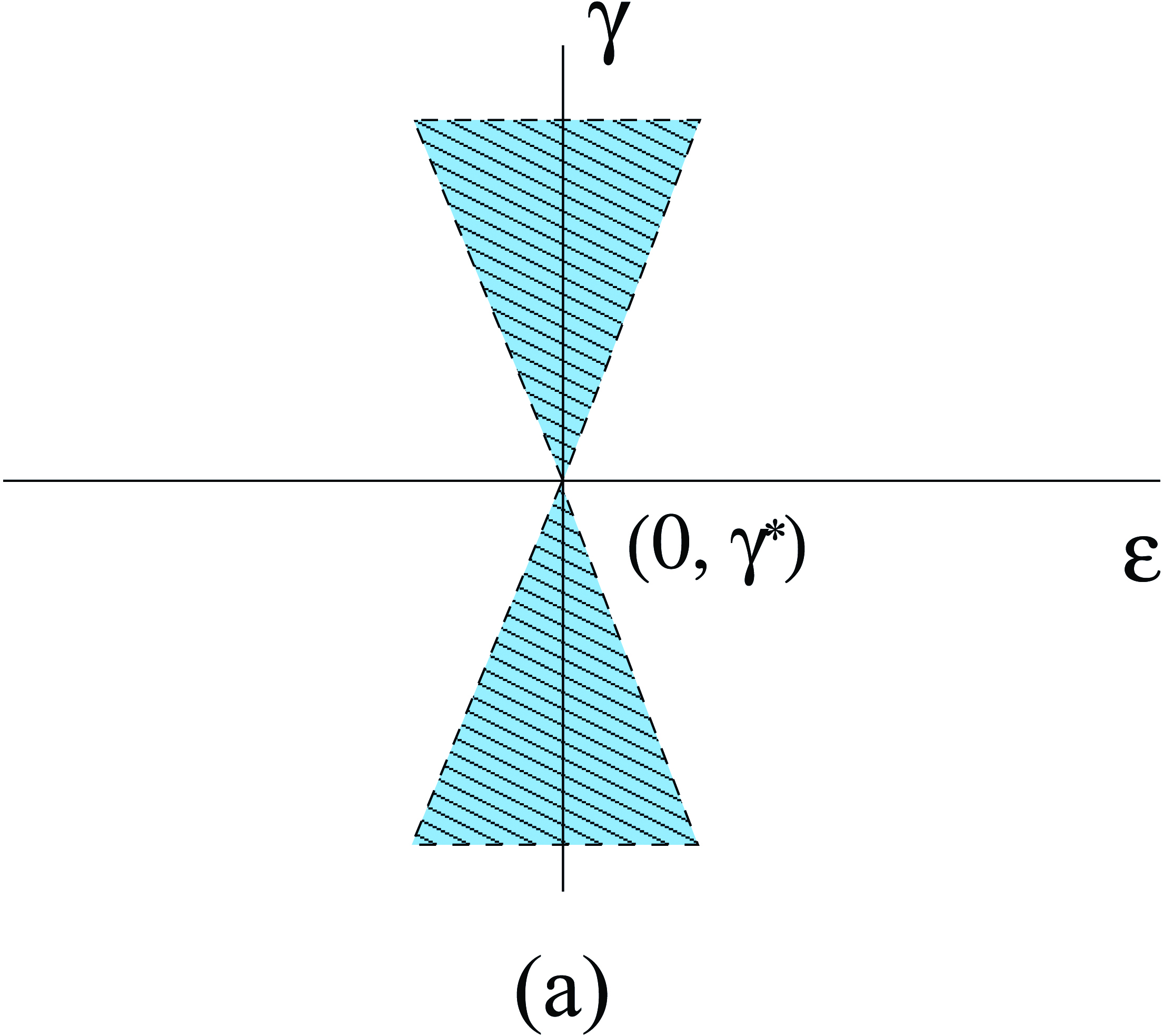
where γ is an additional parameter. In this case, M0(t0) and M1(t0), as well as the quantity ε0 asserted by Theorem 2.2, are all functions of γ, which we denote as M0(t0,γ),M1(t0,γ) and ε0(γ), respectively. Under the assumption that M0(t0,γ*)≡0, we would also have limγ→γ*ε0(γ)=0. Consequently, the parameter region over which the existence of transversal homoclinic intersection is checked by using Theorem 2.2, is as the shadowed area depicted in Figure 2 (a) (excluding the line ε=0). Now, combining Theorem 2.3 with the simple fact that transversal homoclinic intersection is persistent under small perturbation, we are able to add a new open region as shown in Figure 2 (b), over which the existence of transversal homoclinic intersection is also checked.
(D) An Example: We use the equation
(2.7)
u
¨
=
u
-
u
3
+
ε
sin
t
⋅
(
γ
u
u
˙
-
u
2
u
˙
)
as an example, in which γ is an additional parameter. To apply Theorems 2.2 and 2.3, we turn equation (2.7) into the form of (2.2). We then calculate M0(t0,γ) by using (2.3), and M1(t0,γ) by using (2.5). The details of this computation and the resulted integrals for M0(t0,γ) and M1(t0,γ) are delivered in Section 5.
M0(t0,γ) affords analytic evaluation. In fact, we have
M
0
(
t
0
,
γ
)
=
π
e
π
/
2
(
1
(
e
π
-
1
)
-
2
2
3
(
e
π
+
1
)
γ
)
sin
t
0
,
from which it follows that M0(t0,γ*)≡0 at γ*=3(eπ+1)/(22(eπ-1)).
To verify the existence of transversal intersection of the stable and the unstable manifold for equation (2.7) at γ=γ*, we need to compute M1(t0,γ*). We obtain
M
1
(
t
0
,
γ
)
=
M
sc
(
γ
)
sin
2
t
0
where Msc(γ) is the sum of a collection of multiple integrals over ℓ(t); its explicit formula is detailed in Section 5.2. These integrals are unlikely to be analytically evaluated. Using Simpson’s rule to numerically evaluate Msc(γ*), we obtain
M
sc
(
γ
*
)
≈
-
5.92
×
10
-
5
.
As a comparison, we also evaluated M0(t0,γ*) at t0=π/4 by using the same numerical process. We obtain
M
0
(
π
/
4
,
γ
*
)
≈
3.42
×
10
-
13
.
Using 10-13 as a reference to zero, we conclude that Msc(γ*)≠0. Consequently, Theorem 2.3 applies to equation (2.7) at γ=3(eπ+1)/(22(eπ-1)).
2.2 High-Order Melnikov Integrals
We now go beyond M0(t0) and M1(t0) to present a comprehensive description on Mk(t0) for all k≥0: they are sums of certain multiple integrals, which we call higher-order Melnikov integrals.
(A) Functions of Integration: With α, β, f(x,y), g(x,y), P(x,y), Q(x,y), and (a(t),b(t)) being given explicitly, we define functions A(s,z), U(s,z), B(s,z), V(s,z) as follows: A prime is used to denote one derivative with respect to s. Let
(2.8)
A
(
s
,
z
)
=
-
1
z
⋅
b
′
(
s
)
𝔽
-
a
′
(
s
)
𝔾
-
z
⋅
(
a
′′
(
s
)
𝔽
+
b
′′
(
s
)
𝔾
)
(
a
′
(
s
)
)
2
+
(
b
′
(
s
)
)
2
+
z
⋅
(
a
′
(
s
)
b
′′
(
s
)
-
b
′
(
s
)
a
′′
(
s
)
)
,
U
(
s
,
z
)
=
-
b
′
(
s
)
ℙ
-
a
′
(
s
)
ℚ
-
z
⋅
(
a
′′
(
s
)
ℙ
+
b
′′
(
s
)
ℚ
)
(
a
′
(
s
)
)
2
+
(
b
′
(
s
)
)
2
+
z
⋅
(
a
′
(
s
)
b
′′
(
s
)
-
b
′
(
s
)
a
′′
(
s
)
)
,
B
(
s
,
z
)
=
1
z
⋅
(
a
′
(
s
)
𝔽
+
b
′
(
s
)
𝔾
(
a
′
(
s
)
)
2
+
(
b
′
(
s
)
)
2
+
z
⋅
(
a
′
(
s
)
b
′′
(
s
)
-
b
′
(
s
)
a
′′
(
s
)
)
-
1
)
,
V
(
s
,
z
)
=
a
′
(
s
)
ℙ
+
b
′
(
s
)
ℚ
(
a
′
(
s
)
)
2
+
(
b
′
(
s
)
)
2
+
z
⋅
(
a
′
(
s
)
b
′′
(
s
)
-
b
′
(
s
)
a
′′
(
s
)
)
,
where
(2.9)
𝔽
=
-
α
⋅
(
a
(
s
)
+
z
b
′
(
s
)
)
+
f
(
a
(
s
)
+
z
b
′
(
s
)
,
b
(
s
)
-
z
a
′
(
s
)
)
,
𝔾
=
β
⋅
(
b
(
s
)
-
z
a
′
(
s
)
)
+
g
(
a
(
s
)
+
z
b
′
(
s
)
,
b
(
s
)
-
z
a
′
(
s
)
)
,
ℙ
=
P
(
a
(
s
)
+
z
b
′
(
s
)
,
b
(
s
)
-
z
a
′
(
s
)
)
,
ℚ
=
Q
(
a
(
s
)
+
z
b
′
(
s
)
b
(
s
)
-
z
a
′
(
s
)
)
.
The functions A(s,z), B(s,z), U(s,z), V(s,z) are from a canonical form of equation (2.2) on Dℓ, which we will derive in Section 3.1. For the moment what matters to us is the fact that all functions listed above are explicitly defined as functions of two new variables (s,z). To obtain functions that define high-order Melnikov integrals, we expand A(s,z), U(s,z), B(s,z), V(s,z) into power series at (s,z)=(t,0). That is to say that we write
A
(
s
,
z
)
=
A
(
t
,
0
)
+
∑
n
+
m
≥
1
A
n
,
m
(
t
)
(
s
-
t
)
n
z
m
,
U
(
s
,
z
)
=
U
(
t
,
0
)
+
∑
n
+
m
≥
1
U
n
,
m
(
t
)
(
s
-
t
)
n
z
m
,
B
(
s
,
z
)
=
B
(
t
,
0
)
+
∑
n
+
m
≥
1
B
n
,
m
(
t
)
(
s
-
t
)
n
z
m
,
V
(
s
,
z
)
=
V
(
t
,
0
)
+
∑
n
+
m
≥
1
V
n
,
m
(
t
)
(
s
-
t
)
n
z
m
.
High-order Melnikov integrals are defined by using {An,m(t),Un,m(t),Bn,m(t),Vn,m(t)}. For a given integer d>0, let
Φ
d
,
A
=
⋃
0
≤
n
+
m
≤
d
{
A
n
,
m
(
t
)
}
,
Φ
d
,
B
=
⋃
0
≤
n
+
m
≤
d
{
B
n
,
m
(
t
)
}
,
Φ
d
,
U
=
⋃
0
≤
n
+
m
≤
d
{
U
n
,
m
(
t
)
}
,
Φ
d
,
V
=
⋃
0
≤
n
+
m
≤
d
{
V
n
,
m
(
t
)
}
.
We also denote
Φ
d
=
Φ
d
,
A
∪
Φ
d
,
B
∪
Φ
d
,
U
∪
Φ
d
,
V
.
(B) Structure Tree: The second element in defining a high-order Melnikov integral is a structure tree. A structure tree of depth d is represented by a tree of d+1 levels. The highest level of this tree is a single root node representing the entire integral to be defined, the next level consists a number of nodes branched out of the root, each is in turn a root node of an integral of depth ≤d-1, and so on until we reach nodes representing an integral of depth zero.
Assume a given tree as above has p nodes in total, which we index as I1,…,Ip from the bottom to the top level, and at a fixed level, from the right to the left. The root node is then Ip. For i≤p, we define the index set C(i) as the collection of all j, such that Ij is a node directly branched out of Ii. To each node Ii we assign the following to its memory: first, an integral variable τi; second, a function fi(t) from Φd where d=d(Ii) is the depth of the subtree rooted at Ii.
(C) Melnikov Integrals of Order p: There are only two Melnikov integrals of order one for the primary stable solution, and they are defined for t≥0 by
I
1
(
t
,
t
0
)
=
∫
t
+
∞
sin
(
τ
1
+
t
0
)
⋅
U
(
τ
1
,
0
)
e
∫
t
τ
1
A
(
τ
,
0
)
𝑑
τ
𝑑
τ
1
and
I
1
(
t
,
t
0
)
=
∫
0
t
sin
(
τ
1
+
t
0
)
⋅
V
(
τ
1
,
0
)
𝑑
τ
1
.
To define a Melnikov integral of order p, we start with a given structure tree as defined in the last paragraph. A Melnikov integral of order pfor stable solutions is then inductively defined as the following:
If fp(t) is in Φd,A, then
I
p
(
t
,
t
0
)
=
∫
t
+
∞
f
p
(
τ
p
)
e
∫
t
τ
p
A
(
τ
,
0
)
𝑑
τ
∏
j
∈
C
(
p
)
I
j
(
τ
p
,
t
0
)
d
τ
p
;
if fp(t) is in Φd,U, then
I
p
(
t
,
t
0
)
=
∫
t
+
∞
sin
(
τ
p
+
t
0
)
⋅
f
p
(
τ
p
)
e
∫
t
τ
p
A
(
τ
,
0
)
𝑑
τ
∏
j
∈
C
(
p
)
I
j
(
τ
p
,
t
0
)
d
τ
p
;
if fp(t) is in Φd,B, then
I
p
(
t
,
t
0
)
=
∫
0
t
f
p
(
τ
p
)
∏
j
∈
C
(
p
)
I
j
(
τ
p
,
t
0
)
d
τ
p
;
if fp(t) is in Φd,V, then
I
p
(
t
,
t
0
)
=
∫
0
t
sin
(
τ
p
+
t
0
)
⋅
f
p
(
τ
p
)
∏
j
∈
C
(
p
)
I
j
(
τ
p
,
t
0
)
d
τ
p
.
Corresponding to every Melnikov integral Ip(t,t0) of order p for the primary stable solution, we also have a Melnikov integral for the primary unstable solution, which is defined by changing all integral bounds that are +∞ in Ip(t,t0) to -∞. To distinguish the two we would write a Melnikov integral for stable solutions as Ip+(t,t0), and the corresponding Melnikov integral for unstable solutions as Ip-(t,t0). Note that in the above, Ip+(t,t0) is defined on t∈[0,+∞), but Ip-(t,t0) is defined on t∈(-∞,0].
Proposition 2.4.
For every integer k≥0, there is a finite collection Λk of high-order Melnikov integrals so that
M
k
(
t
0
)
=
∑
I
∈
Λ
k
(
I
+
(
0
,
t
0
)
-
I
-
(
0
,
t
0
)
)
.
The set Λk is defined in a unique fashion by a computational process detailed in Section 4.
3 Preliminaries
This is a section of technical preparations. In Section 3.1, we derive a canonical form for equation (2.2) on Dℓ. In Section 3.2, we study the properties of the defining functions of the acquired canonical equation.
3.1 Canonical Equation Around Homoclinic Loop
We start by regarding t in ℓ(t)=(a(t),b(t)) not as time, but as a variable that parameterizes the curve ℓ in the (x,y)-space. To distinguish this variable from the time, we replace t by s to re-write the homoclinic loop as ℓ(s)=(a(s),b(s)). We also use primes to represent derivatives with respect to s. We have
(3.1)
F
(
s
)
:=
a
′
(
s
)
=
-
α
a
(
s
)
+
f
(
a
(
s
)
,
b
(
s
)
)
,
G
(
s
)
:=
b
′
(
s
)
=
β
b
(
s
)
+
g
(
a
(
s
)
,
b
(
s
)
)
,
F
′
(
s
)
:=
a
′′
(
s
)
=
[
-
α
+
f
x
(
a
(
s
)
,
b
(
s
)
)
]
F
(
s
)
+
f
y
(
a
(
s
)
,
b
(
s
)
)
G
(
s
)
,
G
′
(
s
)
:=
b
′′
(
s
)
=
g
x
(
a
(
s
)
,
b
(
s
)
)
F
(
s
)
+
[
β
+
g
y
(
a
(
s
)
,
b
(
s
)
]
G
(
s
)
.
We introduce new phase variables (s,z) by letting
(
x
,
y
)
=
ℓ
(
s
)
+
z
(
b
′
(
s
)
,
-
a
′
(
s
)
)
.
That is to say that (s,z) is such that
(3.2)
x
=
x
(
s
,
z
)
:=
a
(
s
)
+
b
′
(
s
)
z
,
y
=
y
(
s
,
z
)
:=
b
(
s
)
-
a
′
(
s
)
z
.
The new variable z is the distance from (x,y) to the homoclinic loop rescaled by L(s)=|(a′(s),b′(s))|-1.
We derive equations for (2.2) in (s,z). Differentiating (3.2), we obtain
d
x
d
t
=
(
a
′
(
s
)
+
b
′′
(
s
)
z
)
d
s
d
t
+
b
′
(
s
)
d
z
d
t
,
d
y
d
t
=
(
b
′
(
s
)
-
a
′′
(
s
)
z
)
d
s
d
t
-
a
′
(
s
)
d
z
d
t
.
Using equation (2.2), we have
(3.3)
(
a
′
(
s
)
+
b
′′
(
s
)
z
)
d
s
d
t
+
b
′
(
s
)
d
z
d
t
=
𝔽
+
ε
sin
t
⋅
ℙ
,
(
b
′
(
s
)
-
a
′′
(
s
)
z
)
d
s
d
t
-
a
′
(
s
)
d
z
d
t
=
𝔾
+
ε
sin
t
⋅
ℚ
,
where 𝔽, 𝔾, ℙ, ℚ are the same as in (2.9). They are
(3.4)
𝔽
=
-
α
⋅
(
a
(
s
)
+
z
b
′
(
s
)
)
+
f
(
a
(
s
)
+
z
b
′
(
s
)
,
b
(
s
)
-
z
a
′
(
s
)
)
,
𝔾
=
β
⋅
(
b
(
s
)
-
z
a
′
(
s
)
)
+
g
(
a
(
s
)
+
z
b
′
(
s
)
,
b
(
s
)
-
z
a
′
(
s
)
)
,
ℙ
=
P
(
a
(
s
)
+
z
b
′
(
s
)
,
b
(
s
)
-
z
a
′
(
s
)
)
,
ℚ
=
Q
(
a
(
s
)
+
z
b
′
(
s
)
b
(
s
)
-
z
a
′
(
s
)
)
.
From (3.3) it follows that
d
z
d
t
=
-
A
(
s
,
z
)
z
-
ε
sin
t
⋅
U
(
s
,
z
)
,
d
s
d
t
=
1
+
B
(
s
,
z
)
z
+
ε
sin
t
⋅
V
(
s
,
z
)
,
where the functions A(s,z), B(s,z), U(s,z), V(s,z) are the same as in (2.8). They are
(3.5)
A
(
s
,
z
)
=
-
1
z
⋅
b
′
(
s
)
𝔽
-
a
′
(
s
)
𝔾
-
z
⋅
(
a
′′
(
s
)
𝔽
+
b
′′
(
s
)
𝔾
)
(
a
′
(
s
)
)
2
+
(
b
′
(
s
)
)
2
+
z
⋅
(
a
′
(
s
)
b
′′
(
s
)
-
b
′
(
s
)
a
′′
(
s
)
)
,
U
(
s
,
z
)
=
-
b
′
(
s
)
ℙ
-
a
′
(
s
)
ℚ
-
z
⋅
(
a
′′
(
s
)
ℙ
+
b
′′
(
s
)
ℚ
)
(
a
′
(
s
)
)
2
+
(
b
′
(
s
)
)
2
+
z
⋅
(
a
′
(
s
)
b
′′
(
s
)
-
b
′
(
s
)
a
′′
(
s
)
)
,
B
(
s
,
z
)
=
1
z
⋅
(
a
′
(
s
)
𝔽
+
b
′
(
s
)
𝔾
(
a
′
(
s
)
)
2
+
(
b
′
(
s
)
)
2
+
z
⋅
(
a
′
(
s
)
b
′′
(
s
)
-
b
′
(
s
)
a
′′
(
s
)
)
-
1
)
,
V
(
s
,
z
)
=
a
′
(
s
)
ℙ
+
b
′
(
s
)
ℚ
(
a
′
(
s
)
)
2
+
(
b
′
(
s
)
)
2
+
z
⋅
(
a
′
(
s
)
b
′′
(
s
)
-
b
′
(
s
)
a
′′
(
s
)
)
,
in which 𝔽, 𝔾, ℙ, ℚ are as in (3.4). Into these formulas we can substitute a′(s) by using F(s), we can substitute b′(s) by using G(s) in (3.1), and so on.
3.2 Properties of Functions in (3.5)
Let t∈(-∞,+∞) be fixed. We expand A(s,z), B(s,z), U(s,z), V(s,z) at (s,z)=(t,0) to obtain
A
(
s
,
z
)
=
A
(
t
,
0
)
+
∑
n
+
m
≥
1
A
n
,
m
(
t
)
(
s
-
t
)
n
z
m
,
U
(
s
,
z
)
=
U
(
t
,
0
)
+
∑
n
+
m
≥
1
U
n
,
m
(
t
)
(
s
-
t
)
n
z
m
,
B
(
s
,
z
)
=
B
(
t
,
0
)
+
∑
n
+
m
≥
1
B
n
,
m
(
t
)
(
s
-
t
)
n
z
m
,
V
(
s
,
z
)
=
V
(
t
,
0
)
+
∑
n
+
m
≥
1
V
n
,
m
(
t
)
(
s
-
t
)
n
z
m
.
The main objective of this subsection is to establish uniform control on An,m(t), Un,m(t), Bn,m(t), Vn,m(t) for all real t (see Corollaries 3.3 and 3.6). Our strategy is to first control the values of A(s,z), U(s,z), B(s,z), V(s,z) on a complex domain for s and z defined by |Im(s)|<h and ∥z∥<r for some small h,r>0. We then use the Cauchy integral formula for derivatives to obtain uniform bounds for An,m(t), Un,m(t), Bn,m(t), Vn,m(t) for all real t.
In the following lemma we let t∈(-∞,+∞). Let s be a complex variable and
B
h
(
t
)
=
{
s
:
∥
s
-
t
∥
<
h
}
,
where h>0 is a small number independent of t. Let (a(s),b(s)) be the complex extension of the real homoclinic solution ℓ(t)=(a(t),b(t)) to Bh(t).
Lemma 3.1.
There exists a K0>0 sufficiently large such that for all |t|>K0 there exists a uniform constant h>0 so that a(s), b(s) are analytic functions on Bh(t). We also have, for s∈Bh(t),
(3.6)
K
0
-
1
a
2
(
t
)
+
b
2
(
t
)
<
∥
a
(
s
)
∥
+
∥
b
(
s
)
∥
<
K
0
a
2
(
t
)
+
b
2
(
t
)
.
Proof.
With the assumption that K0>0 is sufficiently large, this lemma is about the stable and the unstable solutions in a small neighborhood of (x,y)=(0,0), where the unperturbed equation can be linearized. We can find a near identity coordinate transformation, which we denote as
(3.7)
x
=
X
+
∑
j
=
2
+
∞
f
j
(
X
,
Y
)
,
y
=
Y
+
∑
j
=
2
+
∞
g
j
(
X
,
Y
)
,
where fj(X,Y), gj(X,Y) are homogeneous polynomials of degree j in X, Y, such that equation (2.1) is transformed to
d
X
d
t
=
-
α
X
,
d
Y
d
t
=
β
Y
.
Let us also assume that the power series in (3.7) is convergent on |(X,Y)|<2r for some r>0.
First we have for all real t>K0,
(3.8)
a
(
t
)
=
r
e
-
α
(
t
-
t
0
)
+
∑
j
=
2
+
∞
f
j
(
r
e
-
α
(
t
-
t
0
)
,
0
)
,
b
(
t
)
=
∑
j
=
2
∞
g
j
(
r
e
-
α
(
t
-
t
0
)
,
0
)
,
where t0 is such that X(t0)=r,Y(t0)=0. The complex extension of this solution is
(3.9)
a
(
s
)
=
r
e
-
α
(
s
-
t
0
)
+
∑
j
=
2
+
∞
f
j
(
r
e
-
α
(
s
-
t
0
)
,
0
)
,
b
(
s
)
=
∑
j
=
2
∞
g
j
(
r
e
-
α
(
s
-
t
0
)
,
0
)
.
We note that (a(s),b(s)) are analytic functions on Bh(t) as far as eαh<2. From (3.8) we have for all t>K0,
(3.10)
1
2
r
e
-
α
(
t
-
t
0
)
<
a
(
t
)
<
2
r
e
-
α
(
t
-
t
0
)
,
|
b
(
t
)
|
≪
|
a
(
t
)
|
.
From (3.9) we have for all s∈Bh(t),
(3.11)
1
4
|
a
(
t
)
|
<
1
2
r
e
-
α
(
t
-
K
0
)
<
∥
a
(
s
)
∥
<
2
r
e
-
α
(
t
-
K
0
)
<
4
|
a
(
t
)
|
,
∥
b
(
s
)
∥
≪
∥
a
(
s
)
∥
.
Inequality (3.6) follows from (3.10) and (3.11). The proof for t<-K0 is similar. ∎
Let h,r>0 be two small constants independent of ε and t. Let D⊂R2 be such that
D
=
{
(
s
,
z
)
∈
R
2
:
s
∈
(
-
∞
,
+
∞
)
,
|
z
|
<
r
}
.
We also let 𝔻h,r⊂ℂ2 be such that
𝔻
h
,
r
=
{
(
s
,
z
)
∈
ℂ
2
:
Re
(
s
)
∈
(
-
∞
,
+
∞
)
,
|
Im
(
s
)
|
<
h
,
∥
z
∥
<
r
}
.
Lemma 3.2.
The functions A(s,z), B(s,z), U(s,z), V(s,z) are all analytic in s, z on Dh,r. In addition, they are all uniformly bounded on Dh,r in the sense that there exists a constant K>1 so that the C0-norms of all four functions on Dh,r are <K.
Proof.
We substitute a′(s), b′(s), a′′(s), b′′(s) in (3.5) by using (3.1). All four functions have the same denominator, which we re-write as
(
F
2
(
s
)
+
G
2
(
s
)
)
(
1
+
ℐ
2
⋅
z
)
,
where
ℐ
2
:=
F
(
s
)
G
′
(
s
)
-
G
(
s
)
F
′
(
s
)
F
2
(
s
)
+
G
2
(
s
)
.
We have
ℐ
2
=
g
x
(
a
(
s
)
,
b
(
s
)
)
F
2
(
s
)
-
f
y
(
a
(
s
)
,
b
(
s
)
)
G
2
(
s
)
F
2
(
s
)
+
G
2
(
s
)
+
[
α
+
β
+
g
y
(
a
(
s
)
,
b
(
s
)
)
-
f
x
(
a
(
s
)
,
b
(
s
)
]
F
(
s
)
G
(
s
)
F
2
(
s
)
+
G
2
(
s
)
.
Using the equivalent relations established in Lemma 3.1 between a(s), b(s) and a(Re(s)), b(Re(s)), we only need to bound ℐ2 for real s.
Let s be real from this point on in this proof. We note that b(s)∼a2(s) as s→+∞, and a(s)∼b2(s) as s→-∞, implying that ℐ2 is uniformly bounded for all s∈(-∞,+∞). Consequently,
1
+
ℐ
2
⋅
z
is bounded away from zero assuming r>0 is sufficiently small. It then follows that to bound uniformly A, B, U, V, it suffices to balance the small magnitude of F2(s)+G2(s) for large s by similar factors in their respective numerators. To obtain these balancing factors, we expand 𝔽, 𝔾, ℙ, ℚ into power series of z at z=0. Observe that these expansions are actually written in terms of (F(s))k(G(s))n-kzn. If we assume f(0,0)=g(0,0)=P(0,0)=Q(0,0)=0, they start from n=1. Consequently, the factor z-1 in A(s,z), B(s,z) is canceled, and the rest of all coefficients are uniformly bounded as s→±∞ after been divided by F2(s)+G2(s). ∎
Corollary 3.3.
There exists a constant K>0 so that for all t∈(-∞,+∞) we have
|
A
n
,
m
(
t
)
|
,
|
B
n
,
m
(
t
)
|
,
|
U
n
,
m
(
t
)
|
,
|
V
n
,
m
(
t
)
|
<
K
n
+
m
.
Proof.
First we work on A(s,z). We expand A(s,z) as a power series in z to obtain
A
(
s
,
z
)
=
∑
m
=
0
+
∞
A
m
(
s
,
0
)
z
m
.
It then follows, by integrating on ∥z∥=r/2 using the Cauchy integral formula and Lemma 3.2, that
(3.12)
∥
A
m
(
s
,
0
)
∥
<
K
m
.
We then expand Am(s,0) as a power series in s-t on Bh(t) as
A
m
(
s
,
0
)
=
∑
n
=
0
+
∞
A
n
,
m
(
t
)
(
s
-
t
)
n
and, by integrating on |s-t|=h/2 using the Cauchy integral formula and (3.12), we obtain
|
A
n
,
m
(
t
)
|
<
K
n
+
m
for all real t. Note that in this proof we rely on the fact that the domain for s is a horizontal strip around the real s-axis of a fixed height. The proofs for the other functions are similar. ∎
Our next lemma is on A(s,0).
Lemma 3.4.
We have
lim
s
→
+
∞
A
(
s
,
0
)
=
-
(
α
+
β
)
,
lim
s
→
-
∞
A
(
s
,
0
)
=
α
+
β
.
Proof.
It follows from a direct computation that
A
(
s
,
0
)
=
-
[
α
+
β
+
g
y
(
a
(
s
)
,
b
(
s
)
)
-
f
x
(
a
(
s
)
,
b
(
s
)
)
]
[
F
2
(
s
)
-
G
2
(
s
)
]
F
2
(
s
)
+
G
2
(
s
)
+
2
[
f
y
(
a
(
s
)
,
b
(
s
)
)
+
g
x
(
a
(
s
)
,
b
(
s
)
)
]
F
(
s
)
G
(
s
)
F
2
(
s
)
+
G
2
(
s
)
.
As s→+∞, we have b(s)∼a2(s) because the x-axis is the stable direction. It then follows that
G
(
s
)
∼
F
2
(
s
)
as s→+∞, and
lim
s
→
+
∞
A
(
s
,
0
)
=
-
(
α
+
β
)
.
Similarly, as s→-∞, we have
F
(
s
)
∼
G
2
(
s
)
,
and this leads to
lim
s
→
-
∞
A
(
s
,
0
)
=
α
+
β
,
as desired. ∎
We also need a more precise estimate on B(s,z) and V(s,z). Again, for a given real t∈(-∞,+∞), let s be a complex variable and Bh(t)={∥s-t∥<h} for a small h independent of t. We denote
B
1
(
s
,
z
)
=
B
(
s
,
z
)
a
2
(
t
)
+
b
2
(
t
)
,
V
1
(
s
,
z
)
=
V
(
s
,
z
)
a
2
(
t
)
+
b
2
(
t
)
,
where we are also restricted to ∥z∥<r for a small r>0 independent of t.
Lemma 3.5.
The functions B1(s,z), V1(s,z) are analytic on s∈Bh(t), ∥z∥<r, over which we also have
∥
B
1
(
s
,
z
)
∥
,
∥
V
1
(
s
,
z
)
∥
<
K
for some K>0 that is independent of t.
Proof.
Working on B1(s,z), we expand the numerator into a power series of (F(s))k(G(s))n-kzn. Let us start with the terms of n=1, for which the coefficient for B1(s,z) is
(I)
+
(II)
+
(III)
,
where
(I)
=
2
F
(
s
)
G
(
s
)
(
-
α
-
β
+
∂
x
f
(
a
(
s
)
,
b
(
s
)
)
-
g
y
(
a
(
s
)
,
b
(
s
)
)
)
a
2
(
t
)
+
b
2
(
t
)
(
F
2
(
s
)
+
G
2
(
s
)
)
,
(II)
=
-
F
2
(
s
)
(
f
y
(
a
(
s
)
,
b
(
s
)
)
+
g
x
(
a
(
s
)
,
b
(
s
)
)
)
a
2
(
t
)
+
b
2
(
t
)
(
F
2
(
s
)
+
G
2
(
s
)
)
,
(III)
=
G
2
(
s
)
(
f
y
(
a
(
s
)
,
b
(
s
)
)
+
g
x
(
a
(
s
)
,
b
(
s
)
)
)
a
2
(
t
)
+
b
2
(
t
)
(
F
2
(
s
)
+
G
2
(
s
)
)
.
Using the equivalent relations established in Lemma 3.1 between a(s), b(s) and a(t), b(t), we only need to bound these terms for real s.
Let s be real from this point on in this proof. We only need to consider the case when |s| is sufficiently large. Recall that, expanded at (0,0), the functions f(x,y),g(x,y) are of order two and higher. Consequently, ∂yf(a(s),b(s)) and ∂xg(a(s),b(s)) would start with order one terms in a(s), b(s), providing an additional copy of a(s) or b(s) to (II) and (III). It then follows that, as s→±∞, (II) and (III) are uniformly bounded. For (I), the potentially troublesome term is
2
F
(
s
)
G
(
s
)
a
2
(
t
)
+
b
2
(
t
)
(
F
2
(
s
)
+
G
2
(
s
)
)
.
However, b(s)∼a2(s) as s→+∞, and a(s)∼b2(s) as s→-∞. Consequently, this term is also uniformly bounded as s→±∞.
The proof for V1(s,z) is similar. Here we need the assumption that P(x,y), Q(x,y) are of order two and higher at (x,y)=(0,0). ∎
As a direct result from Lemmas 3.1 and 3.5, we have the following corollary.
Corollary 3.6.
There exists a K>0 so that for all t∈(-∞,+∞),
|
B
n
,
m
(
t
)
|
,
|
V
n
,
m
(
t
)
|
<
a
2
(
t
)
+
b
2
(
t
)
⋅
K
n
+
m
.
4 Main Proofs
In Section 3, we introduced new phase variables (s,z) by using
(
x
,
y
)
=
ℓ
(
s
)
+
z
(
b
′
(
s
)
,
-
a
′
(
s
)
)
,
where ℓ(t)=(a(t),b(t)) is the given homoclinic solution of the unperturbed equation (2.1). We obtained new equations for (2.2) in (s,z) as
(4.1)
d
z
d
t
=
-
A
(
s
,
z
)
z
-
ε
sin
t
⋅
U
(
s
,
z
)
,
d
s
d
t
=
1
+
B
(
s
,
z
)
z
+
ε
sin
t
⋅
V
(
s
,
z
)
,
where A(s,z), B(s,z), U(s,z), V(s,z) are as in (3.5). Let (x(t),y(t)) be a solution of equation (2.2). Geometrically, we projected (x(t),y(t))-(a(t),b(t)) into two directions at ℓ(t), one is perpendicular to ℓ and the other is tangential to ℓ. The perpendicular component is z(t), whereas s(t)-t is the tangential component.
We study the solutions of equation (4.1) on
D
ℓ
=
{
|
z
|
<
r
:
s
∈
(
-
∞
,
+
∞
)
}
.
Let (s^(t),z^(t)) be a primary stable solution of equation (4.1) satisfying s^(t0)=0, z^(t0)=z0. The solution (s^(t),z^(t)) is well-defined for all t∈[t0,+∞). Let s(t)=s^(t+t0), z(t)=z^(t+t0). The solution (s(t),z(t)) is well-defined for all t∈[0,+∞), and it is the solution of the equation
(4.2)
d
z
d
t
=
-
A
(
s
,
z
)
z
-
ε
sin
(
t
+
t
0
)
⋅
U
(
s
,
z
)
,
d
s
d
t
=
1
+
B
(
s
,
z
)
z
+
ε
sin
(
t
+
t
0
)
⋅
V
(
s
,
z
)
satisfying s(0)=0, z(0)=z0.
4.1 Integral Equations for the Primary Stable Solution
We introduce one more change of variables for equation (4.2). Let
Z
=
ε
-
1
z
,
S
=
ε
-
1
(
s
-
t
)
.
We have
(4.3)
d
Z
d
t
=
-
A
(
t
+
ε
S
,
ε
Z
)
Z
-
sin
(
t
+
t
0
)
⋅
U
(
t
+
ε
S
,
ε
Z
)
,
d
S
d
t
=
B
(
t
+
ε
S
,
ε
Z
)
Z
+
sin
(
t
+
t
0
)
⋅
V
(
t
+
ε
S
,
ε
Z
)
.
We re-write equation (4.3) as
d
Z
d
t
=
-
A
(
t
,
0
)
Z
-
sin
(
t
+
t
0
)
⋅
U
(
t
,
0
)
-
∑
n
+
m
≥
1
ε
n
+
m
⋅
[
A
n
,
m
(
t
)
S
n
Z
m
+
1
+
sin
(
t
+
t
0
)
⋅
U
n
,
m
(
t
)
S
n
Z
m
]
,
d
S
d
t
=
B
(
t
,
0
)
Z
+
sin
(
t
+
t
0
)
⋅
V
(
t
,
0
)
+
∑
n
+
m
≥
1
ε
m
+
n
[
B
n
,
m
(
t
)
S
n
Z
m
+
1
+
sin
(
t
+
t
0
)
⋅
V
n
,
m
(
t
)
S
n
Z
m
]
.
We have, from the equation for Z,
(4.4)
Z
(
t
)
=
e
-
∫
0
t
A
(
w
,
0
)
𝑑
w
(
Z
0
-
∫
0
t
sin
(
τ
+
t
0
)
⋅
U
(
τ
,
0
)
e
∫
0
τ
A
(
w
,
0
)
𝑑
w
d
τ
-
∑
n
+
m
≥
1
ε
n
+
m
∫
0
t
(
A
n
,
m
(
τ
)
Z
+
sin
(
τ
+
t
0
)
⋅
U
n
,
m
(
τ
)
)
S
n
Z
m
e
∫
0
τ
A
(
w
,
0
)
𝑑
w
d
τ
)
.
We now derive the integral equations for the primary stable solution by letting
(4.5)
Z
0
=
∫
0
+
∞
sin
(
τ
+
t
0
)
⋅
U
(
τ
,
0
)
e
∫
0
τ
A
(
w
,
0
)
𝑑
w
𝑑
t
+
∑
n
+
m
≥
1
ε
n
+
m
∫
0
+
∞
(
A
n
,
m
(
τ
)
Z
+
sin
(
τ
+
t
0
)
⋅
U
n
,
m
(
τ
)
)
S
n
Z
m
e
∫
0
τ
A
(
w
,
0
)
𝑑
w
𝑑
τ
in (4.4). The intuitive reasoning behind this substitution is that Z(t) should be bounded as t→+∞ for a primary stable solution, but the right-hand side of (4.4) would explode if (4.5) is false.
Using (4.5), we obtain the following integral equations for Z(t) and S(t):
(4.6)
Z
(
t
)
=
∫
t
+
∞
sin
(
τ
+
t
0
)
U
(
τ
,
0
)
e
∫
t
τ
A
(
w
,
0
)
𝑑
w
𝑑
τ
+
∑
n
+
m
≥
1
ε
n
+
m
∫
t
+
∞
[
A
n
,
m
(
τ
)
Z
+
sin
(
τ
+
t
0
)
⋅
U
n
,
m
(
τ
)
]
S
n
Z
m
e
∫
t
τ
A
(
w
,
0
)
𝑑
w
𝑑
τ
and
(4.7)
S
(
t
)
=
∫
0
t
sin
(
τ
+
t
0
)
V
(
τ
,
0
)
𝑑
τ
+
∫
0
t
B
(
τ
,
0
)
Z
𝑑
τ
+
∑
n
+
m
≥
1
ε
n
+
m
∫
0
t
[
B
n
,
m
(
τ
)
Z
+
sin
(
τ
+
t
0
)
⋅
V
n
,
m
(
τ
)
]
S
n
Z
m
𝑑
τ
.
4.2 Explicit Computation of the Primary Stable Solution
We move on to solve equations (4.6) and (4.7) by first writing Z(t) and S(t) as formal power series in ε. Let
(4.8)
Z
(
t
)
=
Z
0
(
t
)
+
∑
n
=
1
∞
ε
n
Z
n
(
t
)
,
S
(
t
)
=
S
0
(
t
)
+
∑
n
=
1
∞
ε
n
S
n
(
t
)
.
We substitute (4.8) into (4.6) and (4.7) to recursively determine Zn(t) and Sn(t). This recursive process is well-defined. We have for the zero-th order term,
Z
0
(
t
)
=
∫
t
+
∞
sin
(
τ
+
t
0
)
U
(
τ
,
0
)
e
∫
t
τ
A
(
w
,
0
)
𝑑
w
𝑑
τ
,
S
0
(
t
)
=
∫
0
t
sin
(
τ
+
t
0
)
V
(
τ
,
0
)
𝑑
τ
+
∫
0
t
B
(
τ
,
0
)
Z
0
(
τ
)
𝑑
τ
.
We further observe that Zn(t), for all n>0, is determined by Zj, Sj, j<n, by using (4.6): on the left-hand side, the only term that is of order n is Zn(t), but on the right-hand side, any term involving Zj(t), Sj(t), j≥n, would have to be of order ≥n+1 in ε. Next we use (4.7) to determine Sn(t). It is a function of Zj(t), Sj(t), j<n, and Zn(t). Consequently, Zn(t), Sn(t) are determined inductively by using (4.6) and (4.7) in the order of
Z
0
(
t
)
→
S
0
(
t
)
→
Z
1
(
t
)
→
S
1
(
t
)
→
Z
2
(
t
)
→
⋯
.
Our next proposition claims that the formal power series expansions (4.8) of Z(t), S(t) obtained by using (4.6) and (4.7) are uniformly convergent.
Proposition 4.1.
There exists an ε0>0 such that the power series Z(t), S(t) in (4.8) are uniformly convergent on Iε0=(-ε0,ε0) for all t∈[0,+∞).
Proof.
We use the standard majorant argument to prove this proposition. We look for a function
𝒲
=
W
0
+
∑
n
=
1
∞
W
n
ε
n
so that
|
Z
n
(
t
)
|
,
|
S
n
(
t
)
|
<
W
n
for all n≥0 and all t∈[0,+∞). To find 𝒲, we
replace An,m, Un,m on the right-hand side of (4.6) by using the upper bound offered in Corollary 3.3, and replace Bn,m, Vn,m on the right-hand side of (4.7) by using the upper bound offered in Corollary 3.6. That is to say we replace An,m, Un,m by using Km+n, and Bn,m, Vn,m by using a2(t)+b2(t)⋅Km+n;
replace sin(t+t0) by 1, replace a(t), b(t) by using |a(t)|, |b(t)|;
It follows that the right-hand sides of (4.6) and (4.7) are bounded by a power series in the form of
K
+
ε
n
∑
n
=
1
∞
n
2
K
n
ℐ
⋅
𝒲
n
,
where
ℐ
=
∫
0
+
∞
(
a
2
(
τ
)
+
b
2
(
τ
)
+
e
∫
0
τ
A
(
w
,
0
)
𝑑
w
)
𝑑
τ
<
+
∞
.
In this argument, we see why Corollary 3.6 is needed for Bn,m and Vn,m: the functions An,m, Un,m are always accompanied by the exponential factor e∫A(w,0)𝑑w but Bn,m, Vn,m are without. Here we are forced to rely on a2(t)+b2(t) offered by Corollary 3.6.
It then follows that the right-hand sides of (4.6) and (4.7) are bounded by a power series in the form of
K
1
+
ε
n
∑
n
=
1
∞
K
1
n
+
1
𝒲
n
=
K
1
1
-
K
1
ε
𝒲
.
We can now compute 𝒲 by letting
𝒲
:=
K
1
1
-
K
1
ε
𝒲
,
from which it follows that
𝒲
=
1
-
1
-
4
K
1
2
ε
2
K
1
ε
.
The radius of convergence of the power series expansion of 𝒲 is (4K12)-1 at ε=0. ∎
4.3 Main Proofs
Proposition 4.2.
The unique solution (Z(t),S(t)) of the integral equations (4.6) and (4.7) obtained in Section 4.2 is the primary stable solution.
Proof.
Let (Z(t), S(t)) be as above. By Proposition 4.1, the solutions Z(t), S(t) are uniformly bounded for all real t. Let
Z
0
=
∫
0
+
∞
sin
(
τ
+
t
0
)
⋅
U
(
τ
,
0
)
e
∫
0
τ
A
(
w
,
0
)
𝑑
w
𝑑
t
+
∑
n
+
m
≥
1
ε
n
+
m
∫
0
+
∞
(
A
n
,
m
(
τ
)
Z
+
sin
(
τ
+
t
0
)
⋅
U
n
,
m
(
τ
)
)
S
n
Z
m
e
∫
0
τ
A
(
w
,
0
)
𝑑
w
𝑑
τ
.
Then Z0 is well-defined, and we can re-write (4.6) back as (4.4). ∎
Though we have worked exclusively on the computation of the primary stable solution thus far, all that has been construed can be used to compute the primary unstable solution. Denote the primary stable and the primary unstable solution of equation (4.3) satisfying S(0)=0 as (S+(t),Z+(t)) and (S-(t),Z-(t)), respectively. We note that (S+(t),Z+(t)) is defined for all t≥0, but (S-(t),Z-(t)) is defined for all t≤0. Recall that these are also functions of ε and t0.
We make the dependency on ε and t0 explicit by writing
Z
+
(
t
,
ε
,
t
0
)
=
Z
0
+
(
t
,
t
0
)
+
∑
n
=
1
∞
ε
n
Z
n
+
(
t
;
t
0
)
,
Z
-
(
t
,
ε
,
t
0
)
=
Z
0
-
(
t
,
t
0
)
+
∑
n
=
1
∞
ε
n
Z
n
-
(
t
;
t
0
)
.
We have
D
(
ε
,
t
0
)
=
ε
Z
+
(
0
,
ε
,
t
0
)
-
ε
Z
-
(
0
,
ε
,
t
0
)
.
It then follows that, for all k≥0,
M
k
(
t
0
)
=
Z
k
+
(
0
,
t
0
)
-
Z
k
-
(
0
,
t
0
)
.
Proof of Proposition 2.1.
The uniform convergence of D(ε,t0) is from Proposition 4.1. The analyticity of Mk(t0) in t0 follows from the fact that Mk(t0) is a sum of finite terms, as functions of t0, each of which is in the form of csini1t0cosi2t0, where c is independent of t0. ∎
Proof of Theorems 2.2 and 2.3.
We solve the equation
D
(
ε
,
t
0
)
=
M
0
(
t
0
)
ε
+
M
1
(
t
0
)
ε
2
+
⋯
=
0
.
For ε≠0, this equation is the same as
M
0
(
t
0
)
+
M
1
(
t
0
)
ε
+
⋯
=
0
.
Assume t0* is such that M0(t0*)=0, ∂t0M0(t0*)≠0. By the implicit function theorem, this equation has a unique solution in the form of t0=t0(ε) satisfying t0(0)=t0*. We have in addition
d
d
ε
t
0
(
0
)
=
-
M
1
(
t
0
*
)
∂
t
0
M
0
(
t
0
*
)
.
As a C1-function in ε at ε=0, we have
t
0
(
ε
)
=
t
0
*
+
O
(
ε
)
,
from which it follows that
∂
t
0
D
(
ε
,
t
0
(
ε
)
)
=
ε
(
∂
t
0
M
0
(
t
0
*
)
+
O
(
ε
)
)
≠
0
provided ε≠0 is sufficiently small. This finishes the proof of Theorem 2.2.
For Theorem 2.3 we solve
M
1
(
t
0
)
+
M
2
(
t
0
)
ε
+
⋯
=
0
because M0(t0)≡0. Under the assumption that M1(t0*)=0, ∂t0M1(t0*)≠0, we have a unique solution t0=t0(ε) satisfying
t
0
(
ε
)
=
t
0
*
+
O
(
ε
)
,
from which it follows that
∂
t
0
D
(
ε
,
t
0
(
ε
)
)
=
ε
2
(
∂
t
0
M
1
(
t
0
*
)
+
O
(
ε
)
)
≠
0
,
as desired. ∎
Proof of Proposition 2.4.
We prove that the structure of the high-order Melnikov integrals for Mk are as what was prescribed in Section 2.2. Let q be a given integer. For i≤q, we denote the collection of Melnikov integrals for Zi and Si as ΛZ,i and ΛS,i, respectively. We inductively assume that
Z
i
=
∑
I
∈
Λ
Z
,
i
I
,
S
i
=
∑
I
∈
Λ
S
,
i
I
.
To compute Zq+1, we drop all terms of order q+1 and higher in Z and S to write
Z
=
Z
0
+
ε
Z
1
+
⋯
+
ε
q
Z
q
,
S
=
S
0
+
ε
S
1
+
⋯
+
ε
q
S
q
.
We also drop all terms satisfying n+m>q+1 on the right-hand side of equation (4.6). What is left is a finite sum, of which we pick up those of order εq+1 to obtain Zq+1. We would end up with a finite collection of definite integrals, the integral bound of which is from t to +∞, and the integrand comprises
an exponential factor in the form of e∫A(w,0)𝑑w,
a function in the form of An,m(t) or sin(t+t0)⋅Un,m(t), in which n+m≤q+1,
a list of integrals from ⋃i≤q(ΛZ,i∪ΛS,i).
These are precisely what we used in items (i) and (ii) of Section 2.2 (C) to inductively define Ip(t,t0). Each of the integrals in (iii) is a direct descendant of the root node Iq+1 in the structure tree.
This is, however, only half of the story. The other half is Sq+1, for which we also need to use (4.7) to compute in order to move the induction forward. Integral bounds are now from 0 to t, and the integrand is, firstly, without the exponential factor, and it, secondly, comprises either a copy of Bn,m(t) or sin(t+t0)⋅Vn,m(t) and, thirdly, comprises a list of integrals from ⋃i≤q(ΛZ,i∪λS,i)∪ΛZ,q+1. These are precisely what we used in items (iii) and (iv) of Section 2.2 (C) to define Ip(t,t0). ∎
4.4 Computing M0(t0) and M1(t0)
In this subsection, we derive M0(t0), M1(t0) by using (4.6) and (4.7).
(A) Computation on M0(t0): Letting Z=Z0+(t,t0) on the left-hand side, and ε=0 on the right-hand side of equation (4.6), we obtain
Z
0
+
(
t
,
t
0
)
=
∫
t
+
∞
sin
(
τ
+
t
0
)
⋅
U
(
τ
,
0
)
e
∫
t
τ
A
(
w
,
0
)
𝑑
w
𝑑
τ
.
We re-write τ as τ1 and w as τ to obtain
(4.9)
Z
0
+
(
t
,
t
0
)
=
∫
t
+
∞
sin
(
τ
1
+
t
0
)
⋅
U
(
τ
1
,
0
)
e
∫
t
τ
1
A
(
τ
,
0
)
𝑑
τ
𝑑
τ
1
.
By symmetry, we have
Z
0
-
(
t
,
t
0
)
=
∫
t
-
∞
sin
(
τ
1
+
t
0
)
⋅
U
(
τ
1
,
0
)
e
∫
t
τ
1
A
(
τ
,
0
)
𝑑
τ
𝑑
τ
1
.
It then follows that
M
0
(
t
0
)
=
Z
0
+
(
0
,
t
0
)
-
Z
0
-
(
0
,
t
0
)
=
∫
-
∞
+
∞
sin
(
τ
1
+
t
0
)
⋅
U
(
τ
1
,
0
)
e
∫
0
τ
1
A
(
τ
,
0
)
𝑑
τ
𝑑
τ
1
.
(B) Computation on M1(t0): To compute M1(t0) we start with S0+(t,t0). Letting S=S0+(t,t0) on the left-hand side, and Z=Z0+(τ,t0) and ε=0 on the right-hand side of equation (4.7), we obtain
(4.10)
S
0
+
(
t
,
t
0
)
=
∫
0
t
sin
(
τ
+
t
0
)
⋅
V
(
τ
,
0
)
𝑑
τ
+
∫
0
t
B
(
τ
,
0
)
Z
0
+
(
τ
,
t
0
)
𝑑
τ
.
Note that Z0+(t,t0) represents the first-order deviation of the stable solution from ℓ(t) in the normal direction of ℓ. It is a Melnikov integral of order one. The function S0+(t,t0) is the first-order deviation of the stable solution from ℓ(t) in the tangential direction of ℓ. It is a sum of two integrals. The first is an order one Melnikov integral from V(t,0), the second is a Melnikov integral of order two involving Z0+(t,t0). Following the layout of Section 2.2 (C), we can write this integral as
∫
0
t
B
(
τ
2
,
0
)
[
∫
τ
2
+
∞
sin
(
τ
1
+
t
0
)
⋅
U
(
τ
1
,
0
)
e
∫
τ
2
τ
1
A
(
τ
,
0
)
𝑑
τ
𝑑
τ
1
]
𝑑
τ
2
.
We then compute Z1+(t,t0) by collecting all terms of order ε on the right-hand side of (4.6). In practice we can set
Z
=
Z
0
+
(
τ
,
t
0
)
,
S
=
S
0
+
(
τ
,
t
0
)
on the right-hand side of (4.6). We obtain
Z
1
+
(
t
,
t
0
)
=
∫
t
+
∞
A
0
,
1
(
τ
)
(
Z
0
+
(
τ
,
t
0
)
)
2
e
∫
t
τ
A
(
w
,
0
)
𝑑
w
𝑑
τ
+
∫
t
+
∞
sin
(
τ
+
t
0
)
⋅
U
0
,
1
(
τ
)
Z
0
+
(
τ
,
t
0
)
e
∫
t
τ
A
(
w
,
0
)
𝑑
w
𝑑
τ
+
∫
t
+
∞
A
1
,
0
(
τ
)
Z
0
+
(
τ
,
t
0
)
S
0
+
(
τ
,
t
0
)
e
∫
t
τ
A
(
w
,
0
)
𝑑
w
𝑑
τ
(4.11)
+
∫
t
+
∞
sin
(
τ
+
t
0
)
⋅
U
1
,
0
(
τ
)
S
0
+
(
τ
,
t
0
)
e
∫
t
τ
A
(
w
,
0
)
𝑑
w
𝑑
τ
.
Denote the first integral as 𝒲11,+(t,t0). We re-write τ as τ3 and w as τ to obtain
𝒲
1
1
,
+
(
t
,
t
0
)
=
∫
t
+
∞
A
0
,
1
(
τ
3
)
(
Z
0
+
(
τ
3
,
t
0
)
)
2
e
∫
t
τ
3
A
(
τ
,
0
)
𝑑
τ
𝑑
τ
3
.
We then substitute Z0+(τ3,t0) by using (4.9) to obtain
𝒲
1
1
,
+
(
t
,
t
0
)
=
∫
t
+
∞
A
0
,
1
(
τ
3
)
(
∫
τ
3
+
∞
sin
(
τ
1
+
t
0
)
⋅
U
(
τ
1
,
0
)
e
∫
τ
3
τ
1
A
(
τ
,
0
)
𝑑
τ
𝑑
τ
1
)
2
e
∫
t
τ
3
A
(
τ
,
0
)
𝑑
τ
𝑑
τ
3
.
We note that 𝒲11,+(0,t0) is 𝒲11,+(t0) in (2.6). Do the same for the rest of the integrals on the right-hand side of (4.11), substituting Z0+(t,t0), S0+(t,t0) by using (4.9) and (4.10). With proper indexing of integral variables we would obtain
Z
1
+
(
t
,
t
0
)
=
∑
i
=
1
6
𝒲
i
1
,
+
(
t
,
t
0
)
,
where 𝒲i1,+(0,t0) is 𝒲i1,+(t0) in (2.6). We have in total six Melnikov integrals for Z1+(t,t0) because S0+(τ,t0) is a sum of two. We also have for the unstable solutions,
Z
1
-
(
t
,
t
0
)
=
∑
i
=
1
6
𝒲
i
1
,
-
(
t
,
t
0
)
,
where 𝒲i1,-(t,t0) is obtained from 𝒲i1,+(t,t0) by changing all integral bounds that are +∞ in 𝒲i1,+(t) to -∞. Finally, by definition we have
M
1
(
t
0
)
=
∑
i
=
1
6
(
𝒲
i
1
,
+
(
0
,
t
0
)
-
𝒲
i
1
,
-
(
0
,
t
0
)
)
.
We end this section by noting that there exists no obstacle for us to continue to compute Mk(t0) for all k≥2 by using (4.6) and (4.7). Calculations remain straightforward but the result would be unbearably long to present even for M2(t0).
5 An Example
In this section, we use (2.3) for M0(t0) and (2.5) for M1(t0) to study the periodically perturbed equation
(5.1)
u
¨
=
u
-
u
3
+
ε
sin
t
⋅
(
γ
u
u
˙
-
u
2
u
˙
)
,
where γ is an additional parameter. In particular, we use (2.5) for M1(t0) to verify the existence of transversal intersections of the stable and the unstable manifold at γ=3(eπ+1)/(22(eπ-1)), a degenerate case in which M0(t0)≡0. This section is divided into two subsections: Calculation based on the unperturbed equation is presented in Section 5.1. The rest of the calculation is presented in Section 5.2.
5.1 Calculation Based on the Unperturbed Equation
The unperturbed part of equation (5.1) is
(5.2)
u
¨
=
u
-
u
3
.
For this equation, u(t)=0 is with a homoclinic solution u=c(t), where
c
=
c
(
t
)
:=
2
2
e
t
+
e
-
t
.
We note that c(t)=c(-t) is an even function and c˙(t)=-c˙(-t) is an odd function. Denote v=u˙, and let x=12(u-v), y=12(u+v). We write equation (5.2) in (x,y) as
x
˙
=
-
x
+
f
(
x
,
y
)
,
y
˙
=
y
+
g
(
x
,
y
)
,
where
f
(
x
,
y
)
=
-
g
(
x
,
y
)
=
1
2
(
x
+
y
)
3
.
The point (x,y)=(0,0) is a saddle, at which α=β=1. Let the homoclinic solution be (x,y)=(a(t),b(t)). We have
a
(
t
)
=
1
2
(
c
(
t
)
-
c
˙
(
t
)
)
,
b
(
t
)
=
1
2
(
c
(
t
)
+
c
˙
(
t
)
)
,
f
(
a
(
t
)
,
b
(
t
)
)
=
-
g
(
a
(
t
)
,
b
(
t
)
)
=
1
2
c
3
(
t
)
.
We also have the following:
a˙2(t)+b˙2(t)=12(c˙2+c¨2) is an even function in t;
a˙2(t)-b˙2(t)=-c˙c¨ is an odd function in t;
a˙(t)b˙(t)=14(c˙2-c¨2) is an even function in t.
We now compute A(t,0), B(t,0), A1,0(t), A0,1(t). We have
A
(
t
,
0
)
=
-
2
𝒜
0
(
t
)
c
˙
2
+
c
¨
2
,
B
(
t
,
0
)
=
2
ℬ
0
(
t
)
c
˙
2
+
c
¨
2
,
(5.3)
A
1
,
0
(
t
)
=
A
˙
(
t
,
0
)
,
A
0
,
1
(
t
)
=
-
2
𝒜
1
(
t
)
c
˙
2
+
c
¨
2
+
4
𝒜
0
(
t
)
ℋ
(
t
)
[
c
˙
2
+
c
¨
2
]
2
,
in which we have the following results.
Lemma 5.1.
𝒜
0
(
t
)
=
-
(
2
-
3
c
2
)
c
˙
c
¨
is odd in
t
;
ℬ
0
(
t
)
=
-
1
2
(
2
-
3
c
2
)
(
c
˙
2
-
c
¨
2
)
is even in
t
;
𝒜
1
(
t
)
=
3
2
c
c
˙
c
¨
2
+
3
c
2
(
1
-
3
2
c
2
)
c
˙
c
¨
is odd in
t
;
ℋ(t)=-34c2(c˙2+c¨2)+14[2-3c2](c˙2-c¨2) is even in t.
Proof.
For 𝒜0(t), ℬ0(t), we have
𝒜
0
(
t
)
=
[
α
+
β
+
g
y
(
a
,
b
)
-
f
x
(
a
,
b
)
]
[
a
˙
2
-
b
˙
2
]
-
2
[
f
y
(
a
,
b
)
+
g
x
(
a
,
b
)
]
a
˙
b
˙
=
-
(
2
-
3
c
2
)
c
˙
c
¨
,
ℬ
0
(
t
)
=
(
g
x
(
a
,
b
)
+
f
y
(
a
,
b
)
)
(
b
˙
2
-
a
˙
2
)
-
2
(
α
+
β
+
g
y
(
a
,
b
)
-
f
x
(
a
,
b
)
)
a
˙
b
˙
=
-
1
2
(
2
-
3
c
2
)
(
c
˙
2
-
c
¨
2
)
.
For the function of first order, we have
𝒜
1
(
t
)
=
b
˙
2
[
f
x
x
(
a
,
b
)
b
˙
2
+
f
y
y
(
a
,
b
)
a
˙
2
-
2
f
x
y
(
a
,
b
)
a
˙
b
˙
]
-
a
˙
2
[
g
x
x
(
a
,
b
)
b
˙
2
+
g
y
y
(
a
,
b
)
a
˙
2
-
2
g
x
y
(
a
,
b
)
a
˙
b
˙
]
-
[
(
-
α
+
f
x
(
a
,
b
)
)
2
-
(
β
+
g
y
(
a
,
b
)
)
2
-
(
f
y
(
a
,
b
)
)
2
+
(
g
x
(
a
,
b
)
)
2
]
a
˙
b
˙
+
[
(
-
α
+
f
x
(
a
,
b
)
)
f
y
(
a
,
b
)
+
(
β
+
g
y
(
a
,
b
)
)
g
x
(
a
,
b
)
]
[
a
˙
2
-
b
˙
2
]
=
3
2
c
c
˙
c
¨
2
+
3
c
2
(
1
-
3
2
c
2
)
c
˙
c
¨
,
ℋ
(
t
)
=
g
x
(
a
,
b
)
a
˙
2
-
f
y
(
a
,
b
)
b
˙
2
+
[
α
+
β
+
g
y
(
a
,
b
)
-
f
x
(
a
,
b
)
]
a
˙
b
˙
=
-
3
4
c
2
(
c
˙
2
+
c
¨
2
)
+
1
4
[
2
-
3
c
2
]
(
c
˙
2
-
c
¨
2
)
,
as desired. ∎
We obtain from (5.3) and Lemma 5.1 the following corollary.
Corollary 5.2.
A(t,0)=-A(-t,0) is odd in t, and B(t,0)=B(-t,0) is even in t.
A1,0(t)=A1,0(-t) is even in t, and A0,1(t)=-A0,1(-t) is odd in t.
Let
E
(
t
1
,
t
2
)
:=
e
∫
t
1
t
2
A
(
τ
,
0
)
𝑑
τ
be the exponential factor.
Lemma 5.3.
We have
E
(
t
1
,
t
2
)
=
c
˙
2
(
t
2
)
+
c
¨
2
(
t
2
)
c
˙
2
(
t
1
)
+
c
¨
2
(
t
1
)
.
The function E(t1,t2) is even in both t1 and t2.
Proof.
Using c¨(t)=c(t)-c3(t), we have
c
˙˙˙
(
t
)
=
(
1
-
3
c
2
(
t
)
)
c
˙
(
t
)
.
It then follows that
d
d
t
(
c
˙
2
(
t
)
+
c
¨
2
(
t
)
)
=
2
(
2
-
3
c
2
(
t
)
)
c
˙
(
t
)
c
¨
(
t
)
=
-
2
𝒜
0
(
t
)
.
Consequently,
E
(
t
1
,
t
2
)
=
e
ln
(
c
˙
2
(
t
2
)
+
c
¨
2
(
t
2
)
)
-
ln
(
c
˙
2
(
t
1
)
+
c
¨
2
(
t
1
)
)
=
c
˙
2
(
t
2
)
+
c
¨
2
(
t
2
)
c
˙
2
(
t
1
)
+
c
¨
2
(
t
1
)
.
∎
5.2 Application of Theorems 2.2 and 2.3
We denote v=u˙ and let x=12(u-v), y=12(u+v) to re-write equation (5.1) as
(5.4)
x
˙
=
-
x
+
f
(
x
,
y
)
+
ε
sin
t
⋅
P
(
x
,
y
,
γ
)
,
y
˙
=
y
+
g
(
x
,
y
)
+
ε
sin
t
⋅
Q
(
x
,
y
,
γ
)
,
where
f
(
x
,
y
)
=
-
g
(
x
,
y
)
=
1
2
(
x
+
y
)
3
,
P
(
x
,
y
)
=
-
Q
(
x
,
y
)
=
1
2
[
(
x
+
y
)
2
(
y
-
x
)
-
γ
(
y
2
-
x
2
)
]
.
(A) Functions Determined by P and Q: We have
U
(
t
,
0
)
=
-
2
𝒰
0
(
t
)
c
˙
2
+
c
¨
2
,
V
(
t
,
0
)
=
2
𝒱
0
(
t
)
c
˙
2
+
c
¨
2
,
(5.5)
U
1
,
0
(
t
)
=
U
˙
(
t
,
0
)
,
U
0
,
1
(
t
)
=
-
2
𝒰
1
(
t
)
c
˙
2
+
c
¨
2
+
4
𝒰
0
(
t
)
ℋ
(
t
)
[
c
˙
2
+
c
¨
2
]
2
,
in which the following assertions hold.
Lemma 5.4.
𝒰0(t)=12(c2-cγ)c˙2 is even in t.
𝒱0(t)=-12(c2-cγ)c˙c¨ is odd in t.
𝒰1(t)=12(2c-γ)c˙2c¨+14(-c2+cγ)(c˙2+c¨2)-14(c2-cγ)(c˙2-c¨2)+12(c2-γc)c˙c˙˙˙ is even in t.
Proof.
We start with
P
(
a
,
b
)
=
-
Q
(
a
,
b
)
=
1
2
(
c
2
-
γ
c
)
c
˙
,
P
x
(
a
,
b
)
=
-
Q
x
(
a
,
b
)
=
1
2
[
2
c
c
˙
-
c
2
+
(
c
-
c
˙
)
γ
]
,
P
y
(
a
,
b
)
=
-
Q
y
(
a
,
b
)
=
1
2
[
2
c
c
˙
+
c
2
-
(
c
+
c
˙
)
γ
]
.
We have
𝒰
0
(
t
)
=
b
˙
P
(
a
,
b
)
-
a
˙
Q
(
a
,
b
)
=
1
2
(
c
2
-
c
γ
)
c
˙
2
,
𝒱
0
(
t
)
=
a
˙
P
(
a
,
b
)
+
b
˙
Q
(
a
,
b
)
=
-
1
2
(
c
2
-
c
γ
)
c
˙
c
¨
,
and
𝒰
1
(
t
)
=
P
x
(
a
,
b
)
b
˙
2
+
Q
y
(
a
,
b
)
a
˙
2
-
(
P
y
(
a
,
b
)
+
Q
x
(
a
,
b
)
)
a
˙
b
˙
-
[
a
¨
P
(
a
,
b
)
+
b
¨
Q
(
a
,
b
)
]
=
1
2
(
2
c
-
γ
)
c
˙
2
c
¨
+
1
4
(
-
c
2
+
c
γ
)
(
c
˙
2
+
c
¨
2
)
-
1
4
(
c
2
-
c
γ
)
(
c
˙
2
-
c
¨
2
)
+
1
2
(
c
2
-
γ
c
)
c
˙
c
˙˙˙
,
as desired. ∎
We obtain from (5.5) and Lemma 5.4 the following corollary.
Corollary 5.5.
U(t,0)=U(-t,0) is even in t, and V(t,0)=-V(-t,0) is odd in t.
U1,0(t)=-U1,0(-t) is odd in t, and U0,1(t)=U0,1(-t) is even in t.
(B) Calculating M0(t0): We obtain, by using (2.3), Lemma 5.3 and Lemma 5.4 (i),
M
0
(
t
0
,
γ
)
=
∫
-
∞
+
∞
sin
(
τ
1
+
t
0
)
U
(
t
1
,
0
)
e
∫
0
τ
1
A
(
τ
,
0
)
𝑑
τ
𝑑
τ
1
=
sin
t
0
⋅
(
ℐ
1
c
-
γ
⋅
ℐ
2
c
)
,
where
ℐ
1
c
=
∫
-
∞
+
∞
cos
τ
1
⋅
c
2
(
τ
1
)
c
˙
2
(
τ
1
)
𝑑
τ
1
=
π
e
π
/
2
(
e
π
-
1
)
,
ℐ
2
c
=
∫
-
∞
+
∞
cos
τ
1
⋅
c
(
τ
1
)
c
˙
2
(
τ
1
)
𝑑
τ
1
=
2
2
π
e
π
/
2
3
(
e
π
+
1
)
.
Here ℐ1c and ℐ2c are evaluated by using the residue theorem. Theorem 2.2 (the traditional Melnikov method) applies for all γ except at γ=γ*:=3(eπ+1)/(22(eπ-1)), at which we have M0(t0,γ*)≡0. To verify the existence of transversal homoclinic intersections of equation (5.4) at γ=γ*, we need to move up to compute M1(t0,γ*).
(C) Calculating M1(t0): Using sin(t+t0)=sint0cost+cost0sint, we can extract the dependency of M1(t0,γ) on t0 out of all integral signs to write
M
1
(
t
0
,
γ
)
=
M
ss
(
γ
)
sin
2
t
0
+
M
sc
(
γ
)
sin
2
t
0
+
M
cc
(
γ
)
cos
2
t
0
.
Using the symmetry presented in Corollaries 5.2 and 5.5, we obtain
M
ss
(
γ
)
=
M
cc
(
γ
)
≡
0
.
Consequently,
M
1
(
t
0
)
=
M
sc
(
γ
)
sin
2
t
0
=
∑
i
=
1
6
(
𝒲
i
(
sc
)
+
𝒲
i
(
cs
)
)
sin
2
t
0
,
where
𝒲
1
(
sc
)
=
2
∫
0
+
∞
A
0
,
1
(
τ
3
)
[
∫
τ
3
+
∞
sin
τ
1
⋅
U
(
τ
1
,
0
)
E
(
τ
3
,
τ
1
)
𝑑
τ
1
]
⋅
[
∫
τ
3
+
∞
cos
τ
2
⋅
U
(
τ
2
,
0
)
E
(
τ
3
,
τ
2
)
𝑑
τ
2
]
E
(
0
,
τ
3
)
𝑑
τ
3
,
𝒲
2
(
sc
)
=
∫
0
+
∞
sin
τ
2
⋅
U
0
,
1
(
τ
2
)
[
∫
τ
2
+
∞
cos
τ
1
⋅
U
(
τ
1
,
0
)
E
(
τ
2
,
τ
1
)
𝑑
τ
1
]
E
(
0
,
τ
2
)
𝑑
τ
2
,
𝒲
3
(
sc
)
=
∫
0
+
∞
A
1
,
0
(
τ
3
)
[
∫
0
τ
3
sin
τ
2
⋅
V
(
τ
2
,
0
)
𝑑
τ
2
]
⋅
[
∫
τ
3
+
∞
cos
τ
1
⋅
U
(
τ
1
,
0
)
E
(
τ
3
,
τ
1
)
𝑑
τ
1
]
E
(
0
,
τ
3
)
𝑑
τ
3
,
𝒲
4
(
sc
)
=
∫
0
+
∞
A
1
,
0
(
τ
4
)
(
∫
0
τ
4
B
(
τ
3
,
0
)
[
∫
τ
3
+
∞
sin
τ
1
⋅
U
(
τ
1
,
0
)
E
(
τ
3
,
τ
1
)
𝑑
τ
1
]
𝑑
τ
3
)
⋅
[
∫
τ
4
+
∞
cos
τ
2
⋅
U
(
τ
2
,
0
)
E
(
τ
4
,
τ
2
)
𝑑
τ
2
]
E
(
0
,
τ
4
)
d
τ
4
,
𝒲
5
(
sc
)
=
∫
0
+
∞
sin
τ
2
⋅
U
1
,
0
(
τ
2
)
[
∫
0
τ
2
cos
τ
1
⋅
V
(
τ
1
,
0
)
𝑑
τ
1
]
E
(
0
,
τ
2
)
𝑑
τ
2
,
𝒲
6
(
sc
)
=
∫
0
+
∞
sin
τ
3
⋅
U
1
,
0
(
τ
3
)
(
∫
0
τ
3
B
(
τ
2
,
0
)
⋅
[
∫
τ
2
+
∞
cos
τ
1
⋅
U
(
τ
1
,
0
)
E
(
τ
2
,
τ
1
)
𝑑
τ
1
]
𝑑
τ
2
)
E
(
0
,
τ
3
)
𝑑
τ
3
,
and we obtain 𝒲i(cs) by switching sine and cosine in 𝒲i(sc). Note that all integral functions above are now explicitly in t. As a matter of fact, we have
A
(
t
,
0
)
=
-
2
𝒜
0
(
t
)
c
˙
2
+
c
¨
2
,
B
(
t
,
0
)
=
2
ℬ
0
(
t
)
c
˙
2
+
c
¨
2
,
A
1
,
0
(
t
)
=
A
˙
(
t
,
0
)
=
-
2
𝒜
˙
0
(
t
)
c
˙
2
+
c
¨
2
+
4
𝒜
0
(
t
)
c
¨
(
c
˙
+
c
˙˙˙
)
[
c
˙
2
+
c
¨
2
]
2
,
A
0
,
1
(
t
)
=
-
2
𝒜
1
(
t
)
c
˙
2
+
c
¨
2
+
4
𝒜
0
(
t
)
ℋ
(
t
)
[
c
˙
2
+
c
¨
2
]
2
,
U
(
t
,
0
)
=
-
2
𝒰
0
(
t
)
c
˙
2
+
c
¨
2
,
V
(
t
,
0
)
=
2
𝒱
0
(
t
)
c
˙
2
+
c
¨
2
,
U
1
,
0
(
t
)
=
U
˙
(
t
,
0
)
=
-
2
𝒰
˙
0
(
t
)
c
˙
2
+
c
¨
2
+
4
𝒰
0
(
t
)
c
¨
(
c
˙
+
c
˙˙˙
)
[
c
˙
2
+
c
¨
2
]
2
,
U
0
,
1
(
t
)
=
-
2
𝒰
1
(
t
)
c
˙
2
+
c
¨
2
+
4
𝒰
0
(
t
)
ℋ
(
t
)
[
c
˙
2
+
c
¨
2
]
2
,
in which, by Lemma 5.1,
𝒜
0
(
t
)
=
-
(
2
-
3
c
2
)
c
˙
c
¨
,
𝒜
˙
0
(
t
)
=
6
c
c
˙
2
c
¨
-
(
2
-
3
c
2
)
(
c
¨
2
+
c
˙
c
˙˙˙
)
,
ℬ
0
(
t
)
=
-
1
2
(
2
-
3
c
2
)
(
c
˙
2
-
c
¨
2
)
,
𝒜
1
(
t
)
=
3
2
c
c
˙
c
¨
2
+
3
c
2
(
1
-
3
2
c
2
)
c
˙
c
¨
,
ℋ
(
t
)
=
-
3
4
c
2
(
c
˙
2
+
c
¨
2
)
+
1
4
[
2
-
3
c
2
]
(
c
˙
2
-
c
¨
2
)
,
and by Lemma 5.4,
𝒰
0
(
t
)
=
1
2
(
c
2
-
c
γ
)
c
˙
2
,
𝒰
˙
0
(
t
)
=
1
2
(
2
c
-
γ
)
c
˙
3
+
(
c
2
-
γ
c
)
c
˙
c
¨
,
𝒱
0
(
t
)
=
-
1
2
(
c
2
-
c
γ
)
c
˙
c
¨
,
𝒰
1
(
t
)
=
1
2
(
2
c
-
γ
)
c
˙
2
c
¨
+
1
4
(
-
c
2
+
c
γ
)
(
c
˙
2
+
c
¨
2
)
-
1
4
(
c
2
-
c
γ
)
(
c
˙
2
-
c
¨
2
)
+
1
2
(
c
2
-
γ
c
)
c
˙
c
˙˙˙
.
Finally, we recall
E
(
t
1
,
t
2
)
=
c
˙
2
(
t
2
)
+
c
¨
2
(
t
2
)
c
˙
2
(
t
1
)
+
c
¨
2
(
t
1
)
,
and in all equations above,
c
=
2
2
e
t
+
e
-
t
=
2
sech
(
t
)
,
c
˙
=
-
2
sech
(
t
)
tanh
(
t
)
,
c
¨
=
2
[
sech
(
t
)
-
2
sech
3
(
t
)
]
,
c
˙˙˙
=
-
2
[
1
-
6
sech
2
(
t
)
]
sech
(
t
)
tanh
(
t
)
.
It does not appear possible to analytically evaluate these integrals. Numerical evaluation using Simpson’s rule is, on the other hand, easy to implement based on what is provided here. At γ*=3(eπ+1)/(22(eπ-1)), we obtain
M
sc
(
γ
*
)
≈
-
5.92
×
10
-
5
.
As a comparison, we also evaluated M0(t0,γ*) at t0=π/4. We obtained
M
0
(
π
/
4
,
γ
*
)
≈
3.42
×
10
-
13
.
Using 10-13 as a reference to zero, we conclude that Msc(γ*)≠0. Consequently, Theorem 2.3 applies at γ=3(eπ+1)/(22(eπ-1)). The existence of transversal intersection of the stable and the unstable manifold for equation (5.4) at γ=γ* is verified by using Theorem 2.3.