Initial boundary value problems for the three-dimensional compressible elastic Navier-Stokes-Poisson equations
-
Yong Wang


Abstract
We study the initial-boundary value problems of the three-dimensional compressible elastic Navier-Stokes-Poisson equations under the Dirichlet or Neumann boundary condition for the electrostatic potential. The unique global solution near a constant equilibrium state in H2 space is obtained. Moreover, we prove that the solution decays to the equilibrium state at an exponential rate as time tends to infinity. This is the first result for the three-dimensional elastic Navier-Stokes-Poisson equations under various boundary conditions for the electrostatic potential.
1 Introduction
As is known to all, solids have elastic behaviors so that the deformations happened in solids recover once the stress field is removed, however, fluids possess the viscous property which plays a role of internal frictions to dissipate the kinetic energy of fluids. Viscoelastic fluids we concern here lie between elastic solids and viscous fluids, which flow like fluids and demonstrate elastic behaviors. This kind of fluids often have more complex microstructures than usual fluids (eg. water and air). A typical example is a polymer containing a large number of long-chain molecules. When these long-chain molecules are stretched out due to flow, an elastic stress will appear to hinder the stretched deformations. In general, there are three kinds of stresses in viscoelastic fluids: the hydrostatic pressure P, the viscous stress
where
To derive a PDE’s model to describe the dynamics of the compressible viscoelastic electrical conducting fluids, we start from the following energy dissipation law: (x, t) ∈ Ω × ℝ+ (Ω⊂ℝ3),
where
The electric energy is only generated by the electrostatic field Es≔ −∇ϕ;
The dissipation is only caused by the fluid viscosity;
The viscosity is chosen to follow Newton’s law of viscosity.
where ⊗ denotes the tensor product. Next one should figure out what is the total stress
from where one can know that
and the pressure P is determined by an ODE:
In the above, the superscript T denotes the transpose of the matrix. Coupled (1.2) with the continuity equation for ρ, the transport equations for
We say that such a system (1.4) is thermodynamically consistent and the constitutive relations for stresses in (1.4) satisfy the principle of material frame indifference. To illustrate those two points, we simply recall the derivation of the system (1.4). Based on the first and second laws of thermodynamics, by assuming that the flow is isothermal and not affected by external forces, we can deduce the formal energy dissipation law as follows. It holds that
where the symbols
where
To be precise, we will study the initial-boundary value problems of the compressible elastic Navier-Stokes-Poisson equations:
with the initial and boundary conditions
and
Here, Ω⊂ℝ3 is a bounded region and ν is the unit outward normal to ∂Ω. The unknown variables ρ=ρ(x, t) > 0, u=u(x, t) ∈ ℝ3,
Here we make an emphasis on physical meanings of the above boundary conditions. The vanishing velocity u on the boundary can be well understood as the non-slip boundary condition due to the fluid viscosity. The homogeneous Dirichlet-type boundary condition for the electrostatic potential ϕ implies that the boundary is grounded. In addition, the homogeneous Neumann-type boundary condition means that the boundary is well-insulated.
Now we review the history on the non-conducting viscoelastic system corresponding to the equations (1.6):
About the Cauchy problem of the system (1.9), Hu and Wang [13] proved the local existence and uniqueness of the strong solution with large initial data. Later, Hu and Wu [17] generalized the local unique strong solution to the global one in the framework of Matsumura and Nishida [34, 35] and got the optimal time-decay rates of lower-order spatial derivatives via semigroup methods developed in [9,39] under the condition that the initial data belong to L1(ℝ3). Based on the same L1 assumption for the initial data, the optimal time-decay rates of higher-order spatial derivatives were obtained by Li et al. [29] who used the Fourier splitting method (cf. [43,44]). Under the weaker assumption in the sense that one replaces L1(ℝ3) with the homogeneous Besov space
Without considering the elasticity, the system (1.6) becomes the compressible Navier-Stokes-Poisson equations:
For the Cauchy problem of the system (1.10), there are a lot of results, cf. [2,8,10,28,47,50,51,52,54] and the references therein. In a sense, the initial-boundary value problem of the Navier-Stokes-Poisson system is more difficult than its Cauchy problem. For initial-boundary value problems, it is necessary to estimate the boundary integral terms involving higher-order derivatives, however, these terms are often out of control due to the loss of the boundary information of derivatives. This means that one cannot obtain higher-order energy estimates by the usual energy methods. An effective method was introduced by Matsumura and Nishida [36,37] to deal with the initial-boundary value problems of the Navier-Stokes equations. However, the Poisson term ρ∇ϕ brings essential difficulties when considering the initial-boundary value problem of the system (1.10). The reason is that one cannot obtain the dissipation estimates of the electric field −∇ϕ whenever the boundary condition for the electrostatic potential is Dirichlet-type or Neumann-type or other else. Given this point, it is not like the Cauchy problem, where the electric field enhances the decay of the density if adding some additional restrictions to the initial electric field, cf. [51]. However, we found a very interesting phenomenon. Under the influence of the elasticity, we can obtain the effective dissipation estimates of ∇ϕ so that the Dirichlet or Neumann boundary value problems can be solved. Very recently, we learn that the Neumann problem for the system (1.10) has been solved by Liu and Zhong [33], while, the Dirichlet problem is still open.
The novelty of this paper mainly includes two points. One is to develop the effects of elasticity variables (not the deformation gradient
Notation. Throughout this paper, we use a ≲ b if a ⩽ Cb for a universal constant C > 0. The relation a ∼ b means that a ≲ b and b ≲ a. We denote the gradient operator
This paper is organized as follows. We make a reformulation for the original problem (1.6)–(1.8) and list the main results in Section 2. In Section 3, we establish the delicate energy estimates of solutions for the linearized system. In Section 4, we complete the proof of Theorem 2.1 by deducing the a priori estimates from the energy estimates in Section 3. In the appendix, we list some auxiliary lemmas needed in the previous sections.
2 Main results
In this section, we first make a reformulation of the original problem and then state the main results on the existence, uniqueness and large-time behaviors (exponential decay rates) of solutions.
2.1 Reformulation
We denote x as the current spatial (Eulerian) coordinate and X as the material (Lagrangian) coordinate for fluid particles. These two coordinates are connected by the flow map x(X, t) defined by the following system of ordinary differential equations:
where u(x (X, t), t) is a given velocity field. Then the deformation gradient
When considering it in the Eulerian coordinate, the deformation gradient
By the chain rule, we easily prove that
Next, we will reformulate the system (1.6). We introduce the inverse of
where X=X(x, t) is the inverse mapping of x(X, t). We define the quantity
which was first introduced by Sideris and Thomases [45]. Note that the matrix
Due to u∣∂Ω=0, it holds that φ∣∂Ω=0. By (2.1)–(2.2) and the Taylor’s expansion, we have
where the absolute convergence of the matrix series is insured due to
Through the fact
which implies
Next, we define the material derivative
Applying the divergence ∇· to both sides of (2.3), we have
For simplicity, we take P′(1)=1. Thus, using (2.3)–(2.6), we can rewrite (1.6) into the linearized form as
which is subject to the initial and boundary conditions
In the above, we define
Since
By the Taylor’s expansion and (2.6), we get
which infers
2.2 Main results
Our main results are stated in the following: the global existence, uniqueness and exponential decay of solutions.
Theorem 2.1
Let Ω⊂ℝ3 be a bounded domain with
Then there exists a suitably small constant δ0 > 0 such that if
then the initial-boundary value problem (1.6)–(1.8) admits a unique global solution
Furthermore, there exists a constant α>0 such that for all t=0,
where C0 > 0 depends only on the initial data.
Finally, we give some remarks.
Remark 2.1
Since it is hard to impose the boundary conditions for the deformation gradient
Remark 2.2
Given the relations (2.4) and (2.6), we can drop the equations for ρ and
Remark 2.3
In this paper, we try to pursue global-in-time solutions with minimal regularity. In fact, the global H2-regularity solution obtained in Theorem 2.1 can become more regular if improving the smoothness of the boundary ∂Ω and the initial data.
Remark 2.4
We easily deduce the regularity of the electrostatic potential ϕ from Theorem 2.1:
by Lemma A.1 (Poincaré's inequality).
3 Energy estimates
For completeness, we first give the local existence and uniqueness of the strong solution of the problem (1.6)–(1.8) and omit its proof, cf. [22].
Proposition 3.1
Let Ω⊂ℝ3 be a bounded domain with
and
where C1 > 1 is some fixed constant.
To obtain the global-in-time solution of the problem (1.6)–(1.8), we shall make many efforts to derive the a priori estimates. Note that the relations (2.4) and (2.6)
It suffices to derive the energy estimates of the solution (u, φ, ▽ϕ) to the linearized system (2.8).
We assume that for some sufficiently small ϵ>0 and some T > 0,
which implies
We first establish the dissipation estimate for
Lemma 3.1
It holds that
Proof. Integrating the resulting identity u · (L1−R1)−Δφ·(L2−R2)=0 over Ω, integrating by parts and using u∣∂Ω=φ∣∂Ω=0 and (1.8), we obtain
Here we have used the facts
and if ϕ∣∂Ω=0, then
and if ▽ϕ·ν∣∂Ω=0 (implying ▽ϕt·ν∣∂Ω=0), then
Then, noting (2.9), we easily use Hölder’s inequality and Lemmas A.1–A.2 to bound the right-hand side of (3.3) by ϵ∣∣(∇ u, ▽φ, ∇2φ)∣∣2. □
Next, we construct the dissipation estimate for
Lemma 3.2
It holds that
Proof. From
we obtain
We integrate the resulting identity ut·(∂tL1−∂tR1)−Δφt·(∂tL2−∂tR2)=0 over Ω to obtain
Here we have used the facts
and if ϕt∣∂Ω=0, then
and if ∇ϕtt·ν∣∂Ω=0, then
Since
Note that
Then, by (3.6)–(3.7), we can use Hölder’s inequality and Lemmas A.1–A.2 to bound the right-hand side of (3.5) by
The following estimate is very important since it gives the estimate independent of ∇2u for the electric field −∇ϕ.
Lemma 3.3
It holds that
Proof. Multiplying (2.8)1 by −φ and integrating the resulting identity over Ω by parts, by Hölder’s and Cauchy’s inequalities and Lemmas A.1–A.2, we can obtain
Here we have estimated this term in light of different boundary conditions:
(1) If ϕ∣∂Ω=0, by Lemmas A.1–A.2, then
(2) If ∇ϕ·ν∣∂Ω=0, by Lemmas A.1–A.2, then
It is necessary to derive the following estimate so that the energy located under the time derivative contains
Lemma 3.4
It holds that
Proof.By integrating the resulting identity ut × (L1−R1)=0 over Ω, we obtain
By (2.9), Hölder’s inequality and Lemmas A.1–A.2, we easily obtain
Plugging (3.12) into (3.13), by Cauchy’s inequality, we deduce (3.10). □
So far, we have used the above four lemmas to establish the lower-order energy estimates for (u, φ, ϕ). To obtain the estimates of the higher-order derivatives of (u, φ, ϕ), we have to split the estimates into the interior estimates and the estimates near the boundary, cf. [36,37]. We first establish the interior estimates.
Lemma 3.5
Let
Proof.Integrating the identity
where we have computed
Then, by (3.6), Hölder’s and Cauchy’s inequalities and Lemmas A.1–A.2, we can bound the right-hand side of (3.17) by
Note that
By Cauchy’s inequality, we have
Thus we prove (3.13). Integrating the identity
Integrating the identity
where we have computed
Hence, since ϵ≪1, we deduce (3.15) from (3.18). Similarly, we can deduce (3.16) from
Next, we shall construct the estimates of higher-order derivatives of (u, φ, ϕ) near the boundary, where we use a method introduced in [36,37]. The main idea is to straighten the boundary by introducing a suitable coordinate transformation on the restricted domain containing the boundary, thus we can integrate by parts to obtain the desired higher-order energy estimates since the tangential derivatives under new coordinates are always equal to zero on that flat boundary.
We shall choose a finite number of bounded open sets
(1) The surface Θj∩∂Ω is the image of a smooth vector function
where δ is some positive constant independent of j, j=1, 2, ⋅, N.
(2) Any x=(x1, x2, x3) ∈ Θj is expressed as
where
We shall omit the superscript j in what follows for simplicity without causing any misunderstanding. And we define the unit vectors
with
By the Frenet-Serret’s formula (cf. [5]), there exist smooth functions (α1, β1, γ1, α2, β2, γ2) of (y1, y2) satisfying
An easy computation shows that the Jacobian J of the transform (3.19):
We observe that the transform (3.19) is regular through choosing y3 so small that J ⩾ δ/2 from (3.20). Hence, the function ϒ(y)≔ (ϒ1, ϒ2, ϒ3)(y) is invertible. Moreover, the derivatives
where
And we can deduce from (3.21) that
and
Thus, in each Θj, (2.7), (2.8)1 and ∇·φ can be rewritten in the local coordinates (y1, y2, y3) as follows:
where
We denote the tangential derivatives by
where 0 ⩽ k ⩽ 2 and
Next, we will use the following four lemmas (Lemmas 3.6–3.9) to give the energy estimates near the boundary. Then we can obtain the desired higher-order estimates for (u, φ) (Lemma 3.10).
Lemma 3.6
Let
Proof. It is similar to the proof of Lemma 3.5, so we omit it. □
Lemma 3.7
Let
Proof. Integrating the identity
We immediately deduce (3.27) from the above. □
Lemma 3.8
Let
and
where κ+ι=1.
Proof. Applying
In order to eliminate the terms
Multiplying (3.33) by
We easily estimate the right-hand side of (3.34) as follows:
and
Substituting (3.35)–(3.36) into (3.34), we obtain (3.28).
Finally, applying
Lemma 3.9
Let
Proof.. By (2.7) and (2.8)1, we have,
Applying Lemma A.4 to (3.40), we obtain
where we have estimated
From (3.40)1, we deduce,
and
Thus we can deduce (3.37) from (3.41)–(3.43). Similarly, we can obtain
To estimate the term
Then applying Lemma A.4 to (3.45), we obtain
where we have estimated
and
Thus we deduce (3.38)–(3.39) from (3.44) and (3.46). Hence, we complete the proof of Lemma 3.9. □
Now we can use the estimates (3.37)–(3.39) in Lemma 3.9 to derive the desired higher-order dissipation estimates for (u, φ).
Lemma 3.10
Let
Proof. First, we can establish the following estimates:
In fact, applying ∇2 to (2.8)2, multiplying it by ∇2φ and integrating over Ω, we have
Therefore, we obtain (3.50). Similarly we can prove (3.51) and (3.52).
Next, plugging (3.50) ×
We estimate
Plugging (3.54) into (3.53), we deduce (3.47). Similarly, we can deduce (3.48) from (3.51) and (3.38), as well as (3.49) from (3.52) and (3.39). □
4 Proof of Theorem 2.1
In this section, we will establish the a priori estimates based on the lemmas in Section 3. Once we have the a prior estimates, the proof of Theorem 2.1 is natural.
List of Energy Estimates
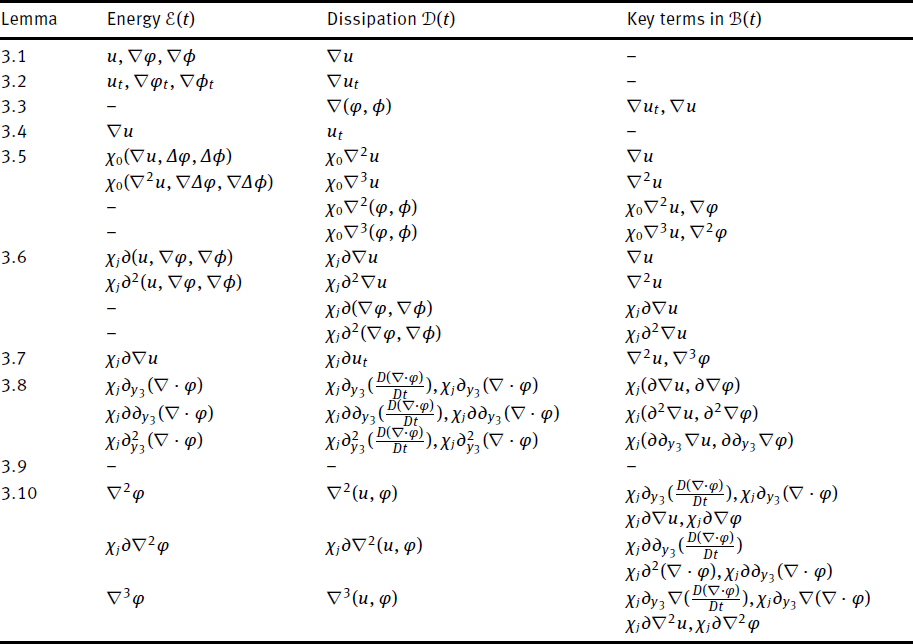 |
Note that the energy estimates obtained in Section 3 are all of form
where
Now, let us do the derivations in detail. Let
Adding (3.10) ×
Applying [(3.15)+(3.16)] ×
Applying [(3.25)+(3.26)]×
Applying (3.47) ×
Applying (3.29)k=1 ×
Applying (3.48) ×
Applying (3.27) ×
We collect all the terms under the time derivative in (4.8) and then denote all of them by Y(t). Then (4.8) becomes
By Poincaré's inequality (cf. Lemma A.1), we easily check that
Applying Gronwall’s inequality to (4.9), we obtain
By (2.8)1, we easily estimate
Combining (4.10)–(4.12) with (3.1), by (2.8), there exists a functional
such that
From the above, we have proved the following a priori estimates:
Proposition 4.1
(A priori estimates). Let T > 0. Assume that for sufficiently small ϵ>0,
Then we have for any t ∈ [0, T] and some α > 0,
where C2 > 1 is some fixed constant.
Then the local solution given in Proposition 3.1 can be extended to the global one by combining the a priori estimates given in Proposition 4.1 with a standard continuous argument, cf. [35]. The exponential decay rate (2.12) follows from (4.13). Hence, we complete the proof of Theorem 2.1.
In the appendix, we list some useful lemmas which are frequently used in previous sections. First, we recall the Poincaré's inequality:
Lemma A.1
Let Ω be a bounded, connected, open subset of ℝn, with a C1 boundary ∂Ω. Assume 1 ⩽ p ⩽ ∞.
(1) If
(2) If u ∈ W1,p(Ω), denoting the average of u over Ω by
The above constant C > 0 depends only on n, p and Ω.
Proof. The detailed proof can be found in [6]. □
Then we recall the classical Gagliardo-Nirenberg-Sobolev inequality on a bounded domain.
Lemma A.2
Let Ω be a bounded domain of ℝn with a Cm boundary ∂Ω. Assume u ∈ Lq(Ω) and ∇mu ∈ Lp(Ω) with 1 ⩽ p, q ⩽ ∞ and
where
with
The above two positive constants C1 and C2 depend only on n, m, k, p, q, α and Ω.
A special case: If u ∈ Wm, p(Ω)∩ Lq(Ω), then we have
Proof. See [38]. □
Next, we give some important time-invariant relations for the density ρ and the deformation gradient
Lemma A.3
If the initial data
then ρ and
Proof. The proof can be found in [41]. □
Then, we shall give the regularity estimates for the Stokes problem:
Lemma A.4
For the Stokes problem (A.1) on a bounded region Ω with ∂Ω ∈ C3, we have
for k=0, 1.
Proof. Refer to [48]. □
Acknowledgements
Wenpei Wu would like to thank Professor Guochun Wu for several helpful discussions on this topic.
Yong Wang was partially supported by Guangdong Provincial Pearl River Talents Program (No. 2017GC010407), Guangdong Province Basic and Applied Basic Research Fund (Nos. 2021A1515010235 and 2020B1515310002), Guangzhou City Basic and Applied Basic Research Fund (No. 202102020436), the NSF of China (No. 11701264) and Science and Technology Program of Guangzhou (No. 2019050001).
-
Conflict of Interest: The authors declare that they have no conflict of interest.
References
[1] H. W. Alt. The entropy principle for interfaces. Fluids and solids. Adv. Math. Sci. Appl., 19(2009), no.2, 585-663.Search in Google Scholar
[2] Q. Y. Bie, Q. R. Wang, and Z. A. Yao. Optimal decay rate for the compressible Navier-Stokes-Poisson system in the critical Lp framework. J. Differential Equations, 263(2017), no.12, 8391-8417.10.1016/j.jde.2017.08.041Search in Google Scholar
[3] Q. Chen and G. C. Wu. The 3D compressible viscoelastic fluid in a bounded domain. Commun. Math. Sci., 16(2018), no.5, 1303-1323.10.4310/CMS.2018.v16.n5.a6Search in Google Scholar
[4] Y. M. Chen and P. Zhang. The global existence of small solutions to the incompressible viscoelastic fluid system in 2 and 3 space dimensions. Comm. Partial Differential Equations, 31(2006), no.10-12, 1793-1810.10.1080/03605300600858960Search in Google Scholar
[5] M. P. do Carmo. Differential Geometry of Curves & Surfaces. Dover Publications, Inc., Mineola, NY, 2016. Revised & updated second edition of [ MR0394451].Search in Google Scholar
[6] L. C. Evans. Partial Differential Equations, volume 19 of Graduate Studies in Mathematics. American Mathematical Society, Providence, RI, second edition, 2010.10.1090/gsm/019Search in Google Scholar
[7] Y. Guo and Y. J. Wang. Decay of dissipative equations and negative Sobolev spaces. Comm. Partial Differential Equations, 37(2012), no.12, 2165-2208.10.1080/03605302.2012.696296Search in Google Scholar
[8] C. C. Hao and H. L. Li. Global existence for compressible Navier-Stokes-Poisson equations in three and higher dimensions. J. Differential Equations, 246(2009), no.12, 4791-4812.10.1016/j.jde.2008.11.019Search in Google Scholar
[9] D. Hoff and K. Zumbrun. Multi-dimensional diffusion waves for the Navier-Stokes equations of compressible flow. Indiana Univ. Math. J., 44(1995), no.2, 603-676.10.1512/iumj.1995.44.2003Search in Google Scholar
[10] L. Hsiao and H. L. Li. Compressible Navier-Stokes-Poisson equations. Acta Math. Sci. Ser. B (Engl. Ed.), 30(2010), no.6, 1937-1948.10.1016/S0252-9602(10)60184-1Search in Google Scholar
[11] X. P. Hu. Global existence of weak solutions to two dimensional compressible viscoelastic flows. J. Differential Equations, 265(2018), no.7, 3130-3167.10.1016/j.jde.2018.05.001Search in Google Scholar
[12] X. P. Hu and F. H. Lin. Global solutions of two-dimensional incompressible viscoelastic flows with discontinuous initial data. Comm. Pure Appl. Math., 69(2016), no.2, 372-404.10.1002/cpa.21561Search in Google Scholar
[13] X. P. Hu and D. H. Wang. Local strong solution to the compressible viscoelastic flow with large data. J. Differential Equations, 249(2010), no.5, 1179-1198.10.1016/j.jde.2010.03.027Search in Google Scholar
[14] X. P. Hu and D. H. Wang. Global existence for the multi-dimensional compressible viscoelastic flows. J. Differential Equations, 250(2011), no.2, 1200-1231.10.1016/j.jde.2010.10.017Search in Google Scholar
[15] X. P. Hu and D. H. Wang. Strong solutions to the three-dimensional compressible viscoelastic fluids. J. Differential Equations, 252(2012), no.6, 4027-4067.10.1016/j.jde.2011.11.021Search in Google Scholar
[16] X. P. Hu and D. H. Wang. The initial-boundary value problem for the compressible viscoelastic flows. Discrete Contin. Dyn. Syst., 35(2015), no.3, 917-934.10.3934/dcds.2015.35.917Search in Google Scholar
[17] X. P. Hu and G. C. Wu. Global existence and optimal decay rates for three-dimensional compressible viscoelastic flows. SIAM J. Math. Anal., 45(2013), no.5, 2815-2833.10.1137/120892350Search in Google Scholar
[18] F. Irgens. Rheology and Non-Newtonian Fluids. Springer, Cham, 2014.10.1007/978-3-319-01053-3Search in Google Scholar
[19] F. Jiang, S. Jiang, and G. C. Wu. On stabilizing effect of elasticity in the Rayleigh-Taylor problem of stratified viscoelastic fluids. J. Funct. Anal., 272(2017), no.9, 3763-3824.10.1016/j.jfa.2017.01.007Search in Google Scholar
[20] F. Jiang, G. C. Wu, and X. Zhong. On exponential stability of gravity driven viscoelastic flows. J. Differential Equations, 260(2016), no.10, 7498-7534.10.1016/j.jde.2016.01.030Search in Google Scholar
[21] D. D. Joseph. Fluid Dynamics of Viscoelastic Liquids, volume 84 of Applied Mathematical Sciences. Springer-Verlag, New York, 1990.10.1007/978-1-4612-4462-2Search in Google Scholar
[22] Y.KageiandS.Kawashima. Local solvability of an initial boundary value problem for a quasilinear hyperbolic-parabolic system. J. Hyperbolic Differ. Equ., 3(2006), no.2, 195-232.10.1142/S0219891606000768Search in Google Scholar
[23] R. G. Larson. The Structure and Rheology of Complex Fluids. Oxford University Press, New York, 1999.Search in Google Scholar
[24] Z. Lei. On 2D viscoelasticity with small strain. Arch. Ration. Mech. Anal., 198(2010), no.1, 13-37.10.1007/s00205-010-0346-2Search in Google Scholar
[25] Z. Lei, C. Liu, and Y. Zhou. Global existence for a 2D incompressible viscoelastic model with small strain. Commun. Math. Sci., 5(2007), no.3, 595-616.10.4310/CMS.2007.v5.n3.a5Search in Google Scholar
[26] Z. Lei, C. Liu, and Y. Zhou. Global solutions for incompressible viscoelastic fluids. Arch. Ration. Mech. Anal., 188(2008), no.3, 371-398.10.1007/s00205-007-0089-xSearch in Google Scholar
[27] Z. Lei and Y. Zhou. Global existence of classical solutions for the two-dimensional Oldroyd model via the incompressible limit. SIAM J. Math. Anal., 37(2005), no.3, 797-814.10.1137/040618813Search in Google Scholar
[28] H. L. Li, A. Matsumura, and G. J. Zhang. Optimal decay rate of the compressible Navier-Stokes-Poisson system in ℝ3 Arch. Ration. Mech. Anal., 196(2010), no.2, 681-713.10.1007/s00205-009-0255-4Search in Google Scholar
[29] Y. Li, R. Y. Wei, and Z. A. Yao. Optimal decay rates for the compressible viscoelastic flows. J. Math. Phys., 57(2016), no.11, 111506, 8pp.10.1063/1.4967975Search in Google Scholar PubMed PubMed Central
[30] F. H. Lin, C. Liu, and P. Zhang. On hydrodynamics of viscoelastic fluids. Comm. Pure Appl. Math., 58(2005), no.11, 1437-1471.10.1002/cpa.20074Search in Google Scholar
[31] F. H. Lin and P. Zhang. On the initial-boundary value problem of the incompressible viscoelastic fluid system. Comm. Pure Appl. Math., 61(2008), no.4, 539-558.10.1002/cpa.20219Search in Google Scholar
[32] C. Liu and N. J. Walkington. An Eulerian description of fluids containing visco-elastic particles. Arch. Ration. Mech. Anal., 159(2001), no.3, 229-252.10.1007/s002050100158Search in Google Scholar
[33] H. R. Liu and H. Zhong. Global solutions to the initial boundary problem of 3-D compressible Navier-Stokes-Poisson on bounded domains. Z. Angew. Math. Phys., 72(2021), no.2, 78.10.1007/s00033-021-01469-ySearch in Google Scholar
[34] A. Matsumura and T. Nishida. The initial value problem for the equations of motion of compressible viscous and heat-conductive fluids. Proc. Japan Acad. Ser. A Math. Sci., 55(1979), no.9, 337-342.10.3792/pjaa.55.337Search in Google Scholar
[35] A. Matsumura and T. Nishida. The initial value problem for the equations of motion of viscous and heat-conductive gases. J. Math. Kyoto Univ., 20(1980), no.1, 67-104.10.1215/kjm/1250522322Search in Google Scholar
[36] A. Matsumura and T. Nishida. Initial-boundary value problems for the equations of motion of general fluids. In Computing methods in applied sciences and engineering, V (Versailles, 1981), pages 389-406. North-Holland, Amsterdam, 1982.Search in Google Scholar
[37] A. Matsumura and T. Nishida. Initial-boundary value problems for the equations of motion of compressible viscous and heat-conductive fluids. Comm. Math. Phys., 89(1983), no.4, 445-464.10.1007/BF01214738Search in Google Scholar
[38] L. Nirenberg. On elliptic partial differential equations. Ann. Scuola Norm. Sup. Pisa, 13(1959), 115-162.10.1007/978-3-642-10926-3_1Search in Google Scholar
[39] G. Ponce. Global existence of small solutions to a class of nonlinear evolution equations. Nonlinear Anal., 9(1985), no.5, 399-418.10.1016/0362-546X(85)90001-XSearch in Google Scholar
[40] J. Z. Qian. Initial boundary value problems for the compressible viscoelastic fluid. J. Differential Equations, 250(2011), no.2, 848-865.10.1016/j.jde.2010.07.026Search in Google Scholar
[41] J. Z. Qian and Z. F. Zhang. Global well-posedness for compressible viscoelastic fluids near equilibrium. Arch. Ration. Mech. Anal., 198(2010), no.3, 835-868.10.1007/s00205-010-0351-5Search in Google Scholar
[42] M. Renardy, W. J. Hrusa, and J. A. Nohel. Mathematical Problems in Viscoelasticity, volume 35 of Pitman Monographs and Surveys in Pure and Applied Mathematics. Longman Scientific & Technical, Harlow; John Wiley & Sons, Inc., New York, 1987.Search in Google Scholar
[43] M. E. Schonbek. L2 decay for weak solutions of the Navier-Stokes equations. Arch. Rational Mech. Anal., 88(1985), no.3, 209-222.10.1007/BF00752111Search in Google Scholar
[44] M. E. Schonbek. The Fourier splitting method. In Advances in geometric analysis and continuum mechanics (Stanford, CA, 1993), pages 269-274. Int. Press, Cambridge, MA, 1995.Search in Google Scholar
[45] T. C. Sideris and B. Thomases. Global existence for three-dimensional incompressible isotropic elastodynamics via the incompressible limit. Comm. Pure Appl. Math., 58(2005), no.6, 750-788.10.1002/cpa.20049Search in Google Scholar
[46] Z. Tan, Y. Wang, and W. P. Wu. Mathematical modeling and qualitative analysis of viscoelastic conductive fluids. Anal. Appl. (Singap.), 18(2020), no.6, 1077-1117.10.1142/S0219530520500141Search in Google Scholar
[47] Z. Tan, T. Yang, H. J. Zhao, and Q. Y. Zou. Global solutions to the one-dimensional compressible Navier-Stokes-Poisson equations with large data. SIAM J. Math. Anal., 45(2013), no.2, 547-571.10.1137/120876174Search in Google Scholar
[48] R. Temam. Navier-Stokes Equations. Theory and Numerical Analysis. North-Holland Publishing Co., Amsterdam-New York-Oxford, 1977. Studies in Mathematics and its Applications, Vol. 2.Search in Google Scholar
[49] C. Truesdell and W. Noll. The Non-linear Field Theories of Mechanics. Springer-Verlag, Berlin, third edition, 2004. Edited and with a preface by Stuart S. Antman.10.1007/978-3-662-10388-3Search in Google Scholar
[50] W. K. Wang and Z. G. Wu. Pointwise estimates of solution for the Navier-Stokes-Poisson equations in multi-dimensions. J. Differential Equations, 248(2010), no.7, 1617-1636.10.1016/j.jde.2010.01.003Search in Google Scholar
[51] Y. J. Wang. Decay of the Navier-Stokes-Poisson equations. J. Differential Equations, 253(2012), no.1, 273-297.10.1016/j.jde.2012.03.006Search in Google Scholar
[52] Y. Z. Wang and K. Y. Wang. Asymptotic behavior of classical solutions to the compressible Navier-Stokes-Poisson equations in three and higher dimensions. J. Differential Equations, 259(2015), no.1, 25-47.10.1016/j.jde.2015.01.042Search in Google Scholar
[53] G. C. Wu, Z. S. Gao, and Z. Tan. Time decay rates for the compressible viscoelastic flows. J. Math. Anal. Appl., 452(2017), no.2, 990-1004.10.1016/j.jmaa.2017.03.044Search in Google Scholar
[54] G. J. Zhang, H. L. Li, and C. J. Zhu. Optimal decay rate of the non-isentropic compressible Navier-Stokes-Poisson system in ℝ3 J. Differential Equations, 250(2011), no.2, 866-891.10.1016/j.jde.2010.07.035Search in Google Scholar
[55] T. Zhang and D. Y. Fang. Global existence of strong solution for equations related to the incompressible viscoelastic fluids in the critical Lp framework. SIAM J. Math. Anal., 44(2012), no.4, 2266-2288.10.1137/110851742Search in Google Scholar
© 2021 Yong Wang and Wenpei Wu, published by De Gruyter
This work is licensed under the Creative Commons Attribution 4.0 International License.
Articles in the same Issue
- Editorial
- Editorial to Volume 10 of ANA
- Regular Articles
- Convergence Results for Elliptic Variational-Hemivariational Inequalities
- Weak and stationary solutions to a Cahn–Hilliard–Brinkman model with singular potentials and source terms
- Single peaked traveling wave solutions to a generalized μ-Novikov Equation
- Constant sign and nodal solutions for superlinear (p, q)–equations with indefinite potential and a concave boundary term
- On isolated singularities of Kirchhoff equations
- On the existence of periodic oscillations for pendulum-type equations
- Multiplicity of concentrating solutions for a class of magnetic Schrödinger-Poisson type equation
- Nehari-type ground state solutions for a Choquard equation with doubly critical exponents
- Gradient estimate of a variable power for nonlinear elliptic equations with Orlicz growth
- The structure of 𝓐-free measures revisited
- Solvability of an infinite system of integral equations on the real half-axis
- Positive Solutions for Resonant (p, q)-equations with convection
- Concentration behavior of semiclassical solutions for Hamiltonian elliptic system
- Global existence and finite time blowup for a nonlocal semilinear pseudo-parabolic equation
- On variational nonlinear equations with monotone operators
- Existence results for nonlinear degenerate elliptic equations with lower order terms
- Blow-up criteria and instability of normalized standing waves for the fractional Schrödinger-Choquard equation
- Ground states and multiple solutions for Hamiltonian elliptic system with gradient term
- Positivity of solutions to the Cauchy problem for linear and semilinear biharmonic heat equations
- Convex solutions of Monge-Ampère equations and systems: Existence, uniqueness and asymptotic behavior
- Multiple solutions for critical Choquard-Kirchhoff type equations
- Regularity for sub-elliptic systems with VMO-coefficients in the Heisenberg group: the sub-quadratic structure case
- Inducing strong convergence of trajectories in dynamical systems associated to monotone inclusions with composite structure
- A posteriori analysis of the spectral element discretization of a non linear heat equation
- Liouville property of fractional Lane-Emden equation in general unbounded domain
- Large data existence theory for three-dimensional unsteady flows of rate-type viscoelastic fluids with stress diffusion
- On some classes of generalized Schrödinger equations
- Variational formulations of steady rotational equatorial waves
- On a class of critical elliptic systems in ℝ4
- Exponential stability of the nonlinear Schrödinger equation with locally distributed damping on compact Riemannian manifold
- On a degenerate hyperbolic problem for the 3-D steady full Euler equations with axial-symmetry
- Existence, multiplicity and nonexistence results for Kirchhoff type equations
- Combined effects of Choquard and singular nonlinearities in fractional Kirchhoff problems
- Convergence analysis for double phase obstacle problems with multivalued convection term
- Multiple solutions for weighted Kirchhoff equations involving critical Hardy-Sobolev exponent
- Boundary value problems associated with singular strongly nonlinear equations with functional terms
- Global solvability in a three-dimensional Keller-Segel-Stokes system involving arbitrary superlinear logistic degradation
- Multiplicity and concentration behaviour of solutions for a fractional Choquard equation with critical growth
- Concentration results for a magnetic Schrödinger-Poisson system with critical growth
- Periodic solutions for a differential inclusion problem involving the p(t)-Laplacian
- The concentration-compactness principles for Ws,p(·,·)(ℝN) and application
- Regularity for commutators of the local multilinear fractional maximal operators
- An improvement to the John-Nirenberg inequality for functions in critical Sobolev spaces
- Local versus nonlocal elliptic equations: short-long range field interactions
- Analysis of a diffusive host-pathogen model with standard incidence and distinct dispersal rates
- Blowing-up solutions of the time-fractional dispersive equations
- Fixed point of some Markov operator of Frobenius-Perron type generated by a random family of point-transformations in ℝd
- Non-stationary Navier–Stokes equations in 2D power cusp domain
- Non-stationary Navier–Stokes equations in 2D power cusp domain
- Nontrivial solutions to the p-harmonic equation with nonlinearity asymptotic to |t|p–2t at infinity
- Iterative methods for monotone nonexpansive mappings in uniformly convex spaces
- Optimality of Serrin type extension criteria to the Navier-Stokes equations
- Fractional Hardy-Sobolev equations with nonhomogeneous terms
- New class of sixth-order nonhomogeneous p(x)-Kirchhoff problems with sign-changing weight functions
- On the set of positive solutions for resonant Robin (p, q)-equations
- Solving Composite Fixed Point Problems with Block Updates
- Lions-type theorem of the p-Laplacian and applications
- Half-space Gaussian symmetrization: applications to semilinear elliptic problems
- Positive radial symmetric solutions for a class of elliptic problems with critical exponent and -1 growth
- Global well-posedness of the full compressible Hall-MHD equations
- Σ-Shaped Bifurcation Curves
- On the critical behavior for inhomogeneous wave inequalities with Hardy potential in an exterior domain
- On singular quasilinear elliptic equations with data measures
- On the sub–diffusion fractional initial value problem with time variable order
- Partial regularity of stable solutions to the fractional Geľfand-Liouville equation
- Ground state solutions for a class of fractional Schrodinger-Poisson system with critical growth and vanishing potentials
- Initial boundary value problems for the three-dimensional compressible elastic Navier-Stokes-Poisson equations