Combinatorics of stratified hyperbolic slices
-
Arne Lien

Abstract
We study sets of univariate hyperbolic polynomials that share the same first few coefficients and show that they have a natural combinatorial description akin to that of polytopes. We define a stratification of these sets in terms of root arrangements of hyperbolic polynomials and show that any stratum is either empty, a point or of maximal dimension, and in the latter case we characterise its relative interior. This is used to show that the poset of strata is a graded, atomic and coatomic lattice and to provide an algorithm for computing which root arrangements are realised in these sets of hyperbolic polynomials.
The topic of this article is the study of (canonical) hyperbolic slices which are sets of univariate hyperbolic polynomials that share the same first few coefficients. The motivation to study such sets stems from the article [14], where they were used to provide a new proof of Timofte’s degree and half degree principle for symmetric polynomials. Therefore these sets are deeply connected with the study of multivariate symmetric polynomials.
A natural way of describing the root arrangement of a hyperbolic polynomial is to construct its partition of multiplicities. However, by also considering in which order the roots arise we get a finer description of the polynomial’s root arrangement which we call its composition. We shall see that by using compositions to stratify the set of hyperbolic polynomials, we get a lattice of strata that is graded, atomic and coatomic.
To establish these combinatorial properties of the set of strata we show that the strata are connected to a type of symmetric, real algebraic sets called Vandermonde varieties. This connection allows us to show that the relative interior of a stratum consists of the polynomials with the largest number of distinct roots and that a stratum is either empty, a point or of the generic dimension of a nonempty Vandermonde variety.
We begin in Section 1 by introducing the sets that we study and by defining our stratification. We look into an example of a set of degree 5 hyperbolic polynomials with the same first three coefficients (Figure 1), and we show in Proposition 1.6 that the collection of strata, partially ordered by inclusion, is a lattice.
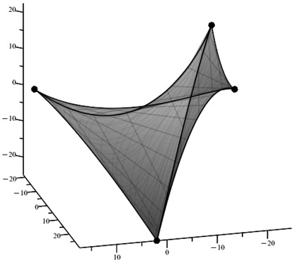
Hyperbolic slice H2(f) for Example 1.4 below
In Section 2 we show that a result from [10] on Vandermonde varieties can be used to describe the relative interior of the strata (Theorem 2.6) and to show that the strata are either empty, a point or of maximal dimension (Theorem 3.10, which says that the poset of strata is a graded, atomic and coatomic lattice. Finally this leads us to Algorithm 3.12 that determines which compositions occur in our sets.
We finish with Section 4 where we discuss how a result from [12] on discriminants and subdiscriminants implies that the boundaries of the sets of hyperbolic polynomials have a concave-like property as exhibited in the picture above. In combination with Theorem 3.10, this leads to the open question of whether hyperbolic slices are concave variations of polytopes.
1 Stratification
We start off by defining hyperbolic slices and showing how we stratify these sets. Then we look closer at the example from the introduction. We finish this section by showing that the collection of strata, partially ordered by inclusion, is a lattice.
Definition 1.1
A univariate polynomial f ∈ ℝ[t] is called hyperbolic if all its roots are real.
Let d be some positive integer throughout this article and let H denote the subset of ℝ[t] consisting of the hyperbolic polynomials of degree d. For f ∈ H we denote by Hs(f) the set of all hyperbolic polynomials of degree d with the same s + 1 first coefficients as f. That is, if
If a = (a1, . . . , ad) are the roots of f, then it is well known that fi = (−1)iei(a) where ei is the ith elementary symmetric polynomial in d variables. Thus the subscript s refers to the number of fixed elementary symmetric polynomials.
Let f be some monic hyperbolic polynomial of degree d ≥ 1 throughout this article. We refer to Hs(f) as a (canonical) hyperbolic slice, where we omit the word canonical as these are the only type of hyperbolic slices we consider. The general definition can be found in [15].
Often a polynomial
To stratify the hyperbolic slices we introduce compositions and a corresponding partial order.
Definition 1.2
A composition of d is a tuple of positive integers, u = (u1, . . . , ul), with
The integers ui are called the parts of u, and ℓ(u) := l is the length of u.
We often use the shorthand (1d) for the composition whose parts are all equal to 1. Also, when nothing further is specified, we let u denote a composition of d.
Definition 1.3
Let u and v be two compositions of a positive integer d. Then v < u if v can be obtained from u by replacing some of the commas in u with plus signs.
To any hyperbolic polynomial f of degree d, we associate a composition of d in the following way: let a1 < a2 ⋅⋅ ⋅ < al be the distinct roots of f with respective multiplicities m1, . . . , ml. Then the composition of f is the tuple v(f) := (m1, . . . , ml), which is a composition of d.
The strata we will look at are given by
Note that
Example 1.4
Let d = 5 and s = 2 and let
If we map the last three coefficients of the polynomials in H2(f), we get the three-dimensional Figure 1 in the introduction. The polynomials with no repeated roots make up the interior, and the strata
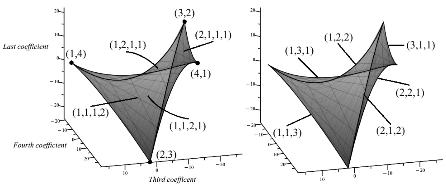
Strata
Next we show that the poset of strata is a lattice. If a and b are elements of a lattice, we denote their join by a ∨ b and their meet by a ∧ b.
Lemma 1.5
The poset of compositions of d is a lattice.
Proof. We prove this by explicitly constructing the join of two compositions u and v of d. Having done so, the existence and uniqueness of the meet is also established since the meet of u and v is just the join of all compositions smaller than both u and v.
If a and b are two compositions of d, note that a ≤ b if and only if
So let M = {u1, u1 + u2, . . . , d} ∪ {v1, v1 + v2, . . . , d} and construct the tuple m = (m1, m2, . . . , ml) containing all the distinct elements of M where mi < mi+1 for any i ∈ [l − 1]; note that ml = d.
Consider the composition w = (m1, m2−m1, m3−m2, . . . , ml−ml−1) of ml = d. Since {u1, u1+u2, . . . , d} ⊆ M and {v1, v1+v2, . . . , d} ⊆ M, we have u ≤ w and v ≤ w. By construction, M is the unique minimal set that contains both {u1, u1 + u2, . . . , d} and {v1, v1 + v2, . . . , d}, hence w is the join of u and v.
From Lemma 1.5 we immediately get that the strata of Hs(f), partially ordered by inclusion, form a lattice. To see this we determine the meet of two strata
so the intersection is a stratum of Hs(f). Thus we have that
and we have shown the following:
Proposition 1.6
The set of strata of Hs(f), partially ordered by inclusion, is a lattice.
However, it is worth pointing out that just because the meet of
A similar problem can arise when we consider joins of strata. However in this case, we shall see in Section 3 that this can be overcome by requiring u and v to be the minimal compositions that can label the strata
Example 1.7
We return to the tetrahedron-like Example 1.4. Let h ∈ H2(f) be a polynomial with composition (2, 3). Then we can see that the compositions occurring in H3(h) are
So the strata labeled by the compositions (1, 1, 3), (2, 1, 2), (2, 2, 1) and (2, 3) are all the same stratum.
For a converse example, consider the stratum labelled by (1, 2, 2). If we look at the join of
However, the minimal composition that can label the stratum
2 Vandermonde varieties
To describe the combinatorial structure of the lattice of strata we need to establish some geometric properties of our strata. In particular, we will show that Arnold’s, Givental’s and Kostov’s work on so-called "Vandermonde varieties" (see [1], [9] and [10]) implies that
To see the connection to their work, let the symmetric group Sym([d]) act on ℝ[x1, . . . , xd] by permuting the variables. It is well known that the elementary symmetric polynomials generate the ring of invariants; see Chapter 7.1 in [6]. The induced action on ℝd permutes the coordinates of the points in ℝd, and the orbit space ℝd/Sym([d]) can be identified with the image of ℝd under the mapping Π : ℝd → H, where
and ei(x) is the ith elementary symmetric polynomial.
Thus the orbit space can be identified with the monic hyperbolic polynomials of degree d, and by restricting Π to the set Kd := {x ∈ ℝd | x1 ≤⋅ ⋅⋅ ≤ xd} we obtain a bijection between Kd and Π(ℝd). So we see that hyperbolic slices can be thought of as sections of the orbit space obtained by intersecting it with certain affine hyperplanes.
Similarly, if u = (u1, . . . , ul) and
where au := (a1, . . . , a1, . . . , al , . . . , al) and ai is repeated ui times. So if we define the real algebraic set
then
Another set of generators for the invariant ring ℝ[x1, . . . , xd]Sym([d]) is the set of all power sums pi(x) :=
To make use of the previous work on Vandermonde varieties, we first need to establish that Πu is a homeomorphism. Note that, as with Hs(f), we equip the sets
Let Bε(a) denote the real open ball about a ∈ ℝk with radius ε > 0, and let
Lemma 2.1
Let ℓ(u) = l, then
is a homeomorphism.
Proof. Note that Πu is a bijection and a polynomial mapping, thus it is a continuous bijection. To see that the inverse map is continuous and that
Let S be a closed subset of
be the inclusion
Let h = td +h1td−1 +⋅ ⋅ ⋅+hd ∉ Πu(S) have the roots a = (a1, . . . , ad) and let hi = fi for all i ∈ [s]. Let ε > 0 be such that Dε(σ(a))∩ ιu(S) is empty for every σ ∈ Sym([d]). If b1, . . . , bk are the distinct roots of h with respective multiplicities v1, . . . , vk, then there is a δ > 0 such that any polynomial g of degree d with |hi − gi | ≤ δ for all i ∈ [d] has exactly vi zeroes in Dε(bi); this statement is proved in [18]. Thus, since Dε(σ(a)) ∩ ιu(S) is empty for any σ ∈ Sym([d]), then so is Bδ(h) ∩ Πu(S), and therefore Πu(S) is closed in ℝd−s. □
Proposition 2.2
The sets
Proof. Firstly, we can use Newton’s identities to define
To see how this proposition can be used to further describe our strata we need some more definitions. First note that as
Definition 2.3
If
the relative interior RelInt
the relative boundary
We can use Proposition 2.2 to describe the relative interior and the relative boundary of our strata and also to determine their dimensions. But the first consequence of the proposition that we need is the following:
Lemma 2.4
If ℓ(u) ≤ s, then
Proof. Suppose that
and so we have
where pi is the ith power sum in d variables and c1, . . . , ck ∈ ℝ are obtained from the numbers −f1, . . . , (−1)k fk using Newton’s identities.
The map F : ℝk → ℝk where F(x) = (p1(xv), . . . , pk(xv)) is a continuously differentiable function whose Jacobian matrix is
Since all the ai’s are distinct, the determinant is nonzero at a. Thus the Jacobian matrix is invertible and by the inverse function theorem, F is invertible on some neighbourhood U of F(a) = (c1, . . . , ck). By Proposition 2.2,
So for any composition w ≤ u that occurs in
Let
denote the projection that forgets the last r coordinates. This map will help us describe the relative interior.
Proposition 2.5
If l = ℓ(u) > s, then the map
is a homeomorphism onto its image and the image is closed in ℝl−s.
Proof. Firstly we consider the case when l = 1; then u = (d) and s = 0. So for any a ∈ ℝ we have that
is essentially just mapping a to −da. This is naturally a homeomorphism and since, by Lemma 2.1, Πu is a homeomorphism, then so is Pd−l. Lastly, since the image of Pd−l is all of ℝ, the image is closed in ℝ.
Next suppose that l ≥ 2. By Lemma 2.4, the polynomials of
To see that the inverse is continuous and that
Let g be a point in the closure of Pd−l(S). Then for any ε > 0, the closed ball
is nonempty. It is also closed since
Since Πu is a homeomorphism, the set
is a closed subset of
So if a ∈ M, then e1(au)≤ g1 − ε and e2(au)≥ g2 − ε since l ≥ 2. Thus, by Newton’s identities, we have
and so M is bounded. Since M is closed and bounded, it is compact.
Since Πu and Pd−l are continuous,
and so Pd−l(S) is closed in ℝl−s. Therefore Pd−l is a closed map and thus Pd−l is a homeomorphism. Lastly, by setting
We see from Lemma 2.5 that when ℓ(u) ≥ s, the largest dimension that
Theorem 2.6
If
Proof. If s = 0 and l = ℓ(u), the map
Next suppose that s > 0 and let
Thus if there is a polynomial
For the reverse inclusion, suppose that l > s so that
By Lemma 2.4 there are only finitely many polynomials in
Since Pd−l(p−) and Pd−l(p+) are interior points of
Thus
and
then
is nonempty but not contractible. This contradicts Proposition 2.2; therefore g cannot be in the relative interior of
Thus if ℓ(u) > s, then the stratum
Theorem 2.7
If ℓ(u) > s and
Proof. If s = 0, then any composition occurs and thus by Theorem 2.3, any stratum is maximal dimensional. Similarly, if s = 1, then for any composition u, the polynomial −e1(xu)− f1 has a real zero with l = ℓ(u) distinct coordinates ordered increasingly. To see this pick l real numbers a1, . . . , al such that a1/u1 < ⋅ ⋅⋅ < al/ul and
let
then
Thus the composition u occurs and
Next we suppose that s ≥ 2. If ℓ(u) ≤ s or
So suppose that
As in the proof of Lemma 2.4, if we define
Since the first k coordinates of a = (a1, . . . , ak+1) are distinct, the determinant does not vanish at
By Lemma 2.4, the one-dimensional manifold U intersects the hyperplane H = {x ∈ ℝk+1 | xk = xk+1} only once. So U must meet the open halfspace H+ := {x ∈ ℝk+1 | xk < xk+1} and thus there is a point in
We can apply the same argument to the polynomial g if v < u, and keep doing this inductively until we find a polynomial with composition u. Then by Theorem 2.6,
Corollary 2.8
Any stratum equals the closure of its relative interior.
Proof. By Theorem 2.7 we may suppose that
Now suppose that the statement is true for all (n − 1)-dimensional strata, where n − 1 ≥ 1. Suppose that
Then by Theorem 2.7 the stratum
3 Combinatorial structure
In this section we explore the combinatorial structure of the lattice of strata and show that this lattice is graded, atomic and coatomic. Then we use this to determine which compositions actually occur in a given hyperbolic slice. Due to Theorem 2.7 we may assume that H s(f) is of dimension d − s > 0 for this section since the one-point lattice trivially satisfies the main combinatorial properties that follow. We begin with the notion of a graded poset.
Definition 3.1
A totally ordered subset of a poset is a chain, and if a chain is maximal with respect to inclusion it is a maximal chain. A poset in which every maximal chain has the same length is called graded.
To see why we call such a poset graded, let y0 < ⋅ ⋅⋅ < yl and z0 < ⋅ ⋅⋅ < zl be two maximal chains of a graded poset L where yi = zj, for some i and j. Then we have i = j, otherwise y0 < y1 < ⋅ ⋅⋅ < yi = zj < zj+1 < ⋅ ⋅⋅ < zl is a maximal chain which is not of length l +1 contradicting the gradedness of L. Thus the rank of yi, rank(yi) := i, is well defined and we can write the poset as the disjoint union
Lemma 3.2
If s ≥ 2 and
Proof. As observed in [14, Proposition 4.1], a stratum of H s(f) is compact when s ≥ 2 since we can rewrite the s first elementary symmetric polynomials in terms of the s first power sums, and the second power sum defines a sphere.
For the second statement, note that when s = 2, the equations
define a nonempty intersection of a hyperplane, whose normal vector is (1, 1, . . . , 1), and a (d − 1)-sphere. This intersection can either be a (d−2)-sphere in the hyperplane, or it can be one of the two points
That is, if v = (d) and the stratum
For s = 0 and s = 1, the hyperbolic slices will have all the main combinatorial properties we are establishing. But the argument is different from the other cases, so we will restrict s to be at least 2 for now. This allows us to use Lemma 3.2, which will be very helpful. Before we proceed note that we use the convention that the empty set has dimension −1.
Proposition 3.3
If s ≥ 2, then the lattice of strata of H s(f) is graded and the rank of a stratum is one more than its dimension.
Proof. If a stratum
Conversely, suppose that
If
If
If
Lastly, if there is an
we have ℓ(u) < ℓ(v) − 1 and so there is a composition w with u < w < v. By Theorem 2.7,
Thus any maximal chain will be at least of length d − s + 1, and so any maximal chain has length d − s + 1. Also, by the above argument any stratum of dimension n ≥ 0 covers a stratum of dimension n − 1, thus its rank must be n + 1. □
Next up is the notion of atomic lattices.
Definition 3.4
In a lattice with smallest element 0, the elements covering 0 are called atoms. The lattice is called atomic if any element can be expressed as the join of atoms.
Lemma 3.5
If s ≥ 2, then for n > 0 any n-dimensional stratum contains at least two distinct (n − 1)-dimensional strata.
Proof. By Proposition 3.3, an n-dimensional stratum
Since
Proposition 3.6
If s ≥ 2, the lattice of strata of Hs(f) is atomic.
Proof. By convention the empty set is the join of an empty set of atoms, and an atom is naturally the join of itself. Also, by Proposition 3.3, the lattice is graded and a stratum’s rank is its dimension plus one, so the atoms are the zero-dimensional strata.
If
Lastly, we look at a sort of converse of atomic lattices called coatomic lattices.
Definition 3.7
In a lattice with largest element 1, the elements covered by 1 are called coatoms. The lattice is called coatomic if any element can be expressed as the meet of coatoms.
Lemma 3.8
If s ≥ 2, then for n < d − s − 1 any n-dimensional stratum is contained in at least two distinct (n + 1)-dimensional strata.
Proof. Let
If n = 0, then
According to Corollary 2.8,
Lastly, if n = −1 then
Proposition 3.9
If s ≥ 2, the lattice of strata of Hs(f) is coatomic.
Proof. The argument is analogous to the proof of Proposition 3.6, just start the induction from the (d − s − 1)-dimensional strata and use Lemma 3.8 instead of Lemma 3.5 for the induction step.
Theorem 3.10
The lattice of strata of H s(f) is graded, atomic and coatomic.
Proof. The only case that remains to check is when s ≤ 1. As we saw in the proof of Theorem 2.7, all compositions occur when s ≤ 1, so the lattice is isomorphic to the lattice of compositions. The lattice of compositions is isomorphic to the face lattice of a (d − 2)-dimensional simplex S. To see this, note that any k + 1 vertices in S determine a k-dimensional face of S.
Similarly there are d − 1 compositions of d of length 2. So if
which is a composition of length k + 2. Thus any bijection from the set of length 2 compositions to the set of vertices of S induces an isomorphism of lattices. Lastly, by items (i) and (v) of Theorem 2.7 in [19], the face lattice of a simplex is graded, atomic and coatomic.
Similar to the case when s ≤ 1, when s = 2 it can be shown that the lattice of strata is isomorphic to the face lattice of a simplex. Although this does not need to be true in general, as can be seen by intersecting H2(f) from Example 1.4 with the affine hyperplane defined by fixing the third coefficient to be 0. This gives us a lattice which is isomorphic to the face lattice of a quadrilateral.
Thus there are examples for which the lattice of strata is not isomorphic to the face lattice of a simplex; however, it would be interesting to find an answer to the following question for general d and s.
Question 3.11
Is the lattice of strata of a hyperbolic slice polytopal?
We finish this section with an algorithm to compute which compositions occur in Hs(f) based on the compositions of length at most s that occur.
Algorithm 3.12
Suppose that Hs(f) is (d − s)-dimensional and that s ≥ 2. Let U denote the set of compositions in Hs(f) of length at most s.
Step 1: Compute the join of every pair of compositions in U:
Step 2: Compute the upward closure of V:
Then U ∪ W is the set of all compositions occurring in H s(f).
Proof. Let w ∈ W; then w ≥ v ∨ u for some v, u ∈ U. Thus both v and u occur in Hs(f) and so
Suppose that a composition u with ℓ(u) > s occurs in Hs(f). Then by Theorem 2.7,
Remark 3.13
Step 1 in Algorithm 3.12 can be accomplished using the method described in Lemma 1.5. That is, the join of u and v can be computed by first constructing the set
Next, construct the tuple (m1, . . . , mk), where the mi’s are distinct, increasingly ordered and {m1, . . . , mk} = M. Then the join of u and v is the composition
However, compositions and our partial order are both implemented in Sage, see [17], so the algorithm can easily be implemented there.
Remark 3.14
As in [1], [9] and [10] we could have focused on the intersection of Vandermonde varieties and K = {x ∈ ℝd | x1 ≤ x2 ≤⋅ ⋅⋅ ≤ xd}. That is, we could consider the set
were w1, . . . , wd ∈ ℝ are positive and c1, . . . , cs ∈ ℝ. If x ∈ M is of the form
When the weights w1, . . . , wd are integers (and by extension rational) then M u is equal to
As we lack the motivation to consider such cases we do not go into details. But the main difference in the arguments would be to use the map Wl : M → ℝl given by
instead of using the map Pd−l ∘ Πu in the proof of Theorem 2.6; otherwise the arguments follow through the same way.
4 A short note on concavity
We will discuss some previously established results on the boundary of hyperbolic slices which, if Question 3.11 is answered in the affirmative, would imply that hyperbolic slices always look like partially deflated polytopes. To do this we start by quickly introducing discriminants and subdiscriminants; more information on these objects can be found in [8] and in Chapter 4 of [2].
Let Δd denote the discriminant of a real, monic, univariate polynomial of degree d. If
This is a real polynomial, symmetric in the roots of g, so it may be written in the elementary symmetric polynomials evaluated at (a1, . . . , ad). That is, the discriminant may be written as a polynomial in the coefficients of the univariate polynomial g, and it vanishes whenever the corresponding univariate polynomial has a repeated root.
Let Z(Δd) ⊆ ℝd denote the real algebraic set given by the discriminant. Then the points of Z(Δd) that correspond to polynomials with a repeated real root split the space of real coefficients into ⌊d/2⌋ regions, each of which is characterised by the number of real roots that the polynomials have.
Similarly, we denote by Δd,k the kth subdiscriminant of a real, monic, univariate polynomial of degree d. The subdiscriminant is defined as
and can also be written as a real polynomial in the coefficients of the univariate polynomial g. We can see that the r first subdiscriminants (including the discriminant) vanish whenever the corresponding univariate polynomial has at most d − r distinct roots.
So if
Naturally the strata of Hs(f) labelled by compositions of length d − k are subsets of Z(Δd,0, . . . , Δd,k). Now suppose that h is hyperbolic and has composition u. Then if the tangent space of
The maximal number of real roots of a polynomial in N is d since h is hyperbolic, thus
Index of notation
[s] = {1, 2, . . . , s}
Hs(f) = {h = td + h1td−1 + ⋅⋅ ⋅ + hd | h is hyperbolic and hi = fi for all i ∈ [s]}
v(h) denotes the composition of h
ℓ(u) denotes the length of the composition u
For x ∈ ℝℓ(u) let
ei(x) is the ith elementary symmetric polynomial in d variables.
pi(x) is the ith power sum in d variables.
Kl = {x ∈ ℝl | x1 ≤⋅ ⋅⋅ ≤ xl}
For x ∈ ℝl let
Bε(a) is the open ball around a ∈ ℝn of radius ε.
u ∨ v denotes the join and u ∧ v denotes the meet of two elements u and v of a lattice.
Funding statement: This work has been supported by the European Union’s Horizon 2020 research and innovation programme under the Marie Sklodowska-Curie Actions, grant agreement 813211 (POEMA).
Acknowledgements
I am very grateful to Claus Scheiderer for all the helpful discussions, critiques and advice along the way. I am also very grateful to Cordian Riener for bringing to my attention some of the literature on the topic and for greatly simplifying the argument behind Theorem 2.7. Lastly I would also like to thank Tobias Metzlaff whose suggestion led to the pretty picture above.
-
Communicated by: M. Hering
References
[1] V. I. Arnol’d, Hyperbolic polynomials and Vandermonde mappings. (Russian) Funktsional. Anal. i Prilozhen. 20 (1986), 52–53. English translation in Funct. Anal. Appl. 20 (1986), 125–127. MR847139 Zbl 0608.5800810.1007/BF01077267Suche in Google Scholar
[2] S. Basu, R. Pollack, M.-F. Roy, Algorithms in real algebraic geometry, volume 10 of Algorithms and Computation in Mathematics. Springer 2006. MR2248869 Zbl 1102.1404110.1007/3-540-33099-2Suche in Google Scholar
[3] S. Basu, C. Riener, Vandermonde varieties, mirrored spaces, and the cohomology of symmetric semi-algebraic sets. Found. Comput. Math. 22 (2022), 1395–1462. MR4498438 Zbl 1497.1411710.1007/s10208-021-09519-7Suche in Google Scholar
[4] J. Bochnak, M. Coste, M.-F. Roy, Real algebraic geometry. Springer 1998. MR1659509 Zbl 0912.14023)10.1007/978-3-662-03718-8Suche in Google Scholar
[5] B. Chevallier, Courbes maximales de Harnack et discriminant. In: Séminaire sur la géométrie algébrique réelle, Tome I, II, volume 24 of Publ. Math. Univ. Paris VII, 41–65, Univ. Paris VII, Paris 1986. MR923547 Zbl 0761.14011Suche in Google Scholar
[6] D. A. Cox, J. Little, D. O’Shea, Ideals, varieties, and algorithms. Springer 2015. MR3330490 Zbl 1335.1300110.1007/978-3-319-16721-3Suche in Google Scholar
[7] J.-P. Dedieu, Obreschkoff’s theorem revisited: what convex sets are contained in the set of hyperbolic polynomials? J. Pure Appl. Algebra 81 (1992), 269–278. MR1179101 Zbl 0772.1200210.1016/0022-4049(92)90060-SSuche in Google Scholar
[8] I. M. Gel’fand, M. M. Kapranov, A. V. Zelevinsky, Discriminants, resultants, and multidimensional determinants. Birkhäuser, Boston, MA 1994. MR1264417 Zbl 0827.1403610.1007/978-0-8176-4771-1Suche in Google Scholar
[9] A. B. Givental’, Moments of random variables and the equivariant Morse lemma. (Russian) Uspekhi Mat. Nauk 42 (1987), no. 2(254), 221–222. English translation in Russ. Math. Surv. 42 (1987), No. 2, 275–276. MR898630 Zbl 0647.5702610.1070/RM1987v042n02ABEH001314Suche in Google Scholar
[10] V. P. Kostov, On the geometric properties of Vandermonde’s mapping and on the problem of moments. Proc. Roy. Soc. Edinburgh Sect. A 112 (1989), 203–211. MR1014650 Zbl 0687.5803010.1017/S0308210500018679Suche in Google Scholar
[11] V. P. Kostov, Topics on hyperbolic polynomials in one variable, volume 33 of Panoramas et Synthèses. Société Mathématique de France, Paris 2011. MR2952044 Zbl 1259.12001Suche in Google Scholar
[12] I. Meguerditchian, Géométrie du discriminant réel et des polynômes hyperboliques. PhD thesis, Univ. Rennes 1, 1991.Suche in Google Scholar
[13] I. Meguerditchian, A theorem on the escape from the space of hyperbolic polynomials. Math. Z. 211 (1992), 449–460. MR1190221 Zbl 0763.5800610.1007/BF02571438Suche in Google Scholar
[14] C. Riener, On the degree and half-degree principle for symmetric polynomials. J. Pure Appl. Algebra 216 (2012), 850–856. MR2864859 Zbl 1242.0527210.1016/j.jpaa.2011.08.012Suche in Google Scholar
[15] C. Riener, R. Schabert, Linear slices of hyperbolic polynomials and positivity of symmetric polynomial functions. Preprint 2023, arXiv 2203.08727Suche in Google Scholar
[16] R. P. Stanley, Enumerative combinatorics. Volume 1. Cambridge Univ. Press 2012. MR2868112 Zbl 1247.05003Suche in Google Scholar
[17] The Sage Developers, SageMath, the Sage Mathematics Software System (Version 9.3), 2021. https://www.sagemath.orgSuche in Google Scholar
[18] D. J. Uherka, A. M. Sergott, On the continuous dependence of the roots of a polynomial on its coefficients. Amer. Math. Monthly 84 (1977), 368–370. MR435434 Zbl 0434.3200310.1080/00029890.1977.11994362Suche in Google Scholar
[19] G. M. Ziegler, Lectures on polytopes. Springer 1995. MR1311028 Zbl 0823.5200210.1007/978-1-4613-8431-1Suche in Google Scholar
© 2025 Walter de Gruyter GmbH, Berlin/Boston
This work is licensed under the Creative Commons Attribution 4.0 International License.
Artikel in diesem Heft
- Frontmatter
- Combinatorics of stratified hyperbolic slices
- Godbersen’s conjecture for locally anti-blocking bodies
- A Hilbert metric for bounded symmetric domains
- On the generalized Suzuki curve
- The partition of PG(2, q3) arising from an order 3 planar collineation
- Well-rounded lattices from odd prime degree number fields in the ramified case
- Split Cayley hexagons via subalgebras of octonion algebras
- Relative Lipschitz saturation of complex algebraic varieties
- The prime grid contains arbitrarily large empty polygons
- The geometry of locally bounded rational functions