A Generic Statistics-Based Tessellation Method of Voronoi Diagram

1 Introduction

Since the Voronoi diagram, a spatial tessellation based on closeness to points in a specific subset of a plane, was put forward by Russian mathematician Voronoi and named after him in 1908[1], a multiple of academicians have conducted deeply researches on it, e.g., Voronoi diagrams — A survey of a fundamental geometric data structure was investigated[2], as well as the research about weighted Voronoi diagrams in raster[3,4]; centroidal Voronoi tessellations on applications and algorithms[5,6]; Bregman Voronoi diagrams with Bregman divergence[7] and the fast dynamic Voronoi treemaps in the application of hierarchical visualization[8]. The investigations about Voronoi, e.g., Voronoi-based dynamic spatial data model[9], a Voronoi-based 9-intersection model for spatial relations[10], Voronoi-based k-order neighbour relations for spatial analysis[11] and an algorithm for the generation of Voronoi diagrams on the sphere based on QTM[12], have a certain academic influence in this field. In addition, the computing spatial relations in GIS were reviewed through Voronoi methods[13], and in order to reduce the complexity of spatial tessellation, a backward inflation generating method for Voronoi diagram based on linear quadtree structure was proposed[14]. The other generating method of Voronoi diagram, for instance, a sweepline algorithm for Euclidean Voronoi diagram by circles was produced[15], and the algorithm for constructing network Voronoi diagram based on flow extension ideas[16] was came up on the network path distance, etc.

First and foremost, from above presentation, it could be seen that most these kinds of methods or algorithms expedite the development of Voronoi diagram undoubtedly in theory and application. However, there are still some certain deficiencies that the generating methods or algorithms are on the ground of Euclidean distance or weighted Euclidean distance based on vector or raster data. From the point of view of uncertainty, the relativity or some distribution that exists in data objectively was not taken into consideration.

Second, the above mentioned Voronoi diagram is onefold and continuous in the neighborhood of generating cell. However, in practice, the adjacent relation in Voronoi cell should certainly exist the phenomenon that one Voronoi diagram crosses the other ones. In other words, although the Voronoi diagram is obstructed by its neighbors, it could originally present a discrete form to keep on extending the action range along its spatial domain.

Hence, on the issues, taking probability and statistics into consideration, this paper aims to give a generic generating method of Voronoi diagram. In remaining parts, Section 2 is focused on the spatial uncertainty that could impact the location distribution of spatial data. In Section 3, compared with ordinary and weighted Voronoi, the general definition of statistical Voronoi diagram is proposed according to Mahalanobis distance function derived from spatial uncertainty. In Section 4, the generating method of general Voronoi is presented by experiments, particularly for the Voronoi cell that is equipped with cross characteristic. In Section 5, discussion and further research are given.

2 Spatial Uncertainty

2.1 Data Uncertainty

The objective world is flooded with occasional events and the spatial entities in it are featured with complexity and variability. The data described normally are far less than the objective ones because the global data are usually approximated by expected values. Furthermore, some certain attributes are determined by adjacent relationship among entities, not by the data per se[17]. Uncertain spatial location means that the location obtained is inconsistent with its real location absolutely, but it could be referred by other entities through spatial relations correspondingly, such as linear reference in GIS. Usually the mean value and covariance are employed to describe the consistency in distribution field[18]. For example, the following Gaussian distribution shown in Figure 1 with one variate[19].

Figure 1

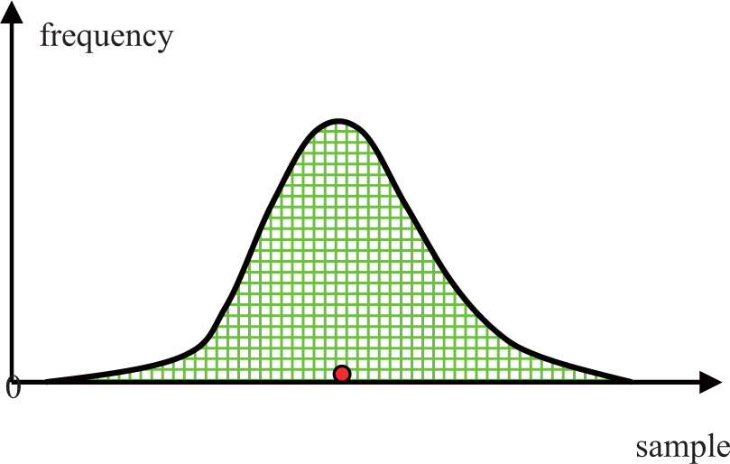
Gaussian distribution by single parameter

Due to the dimensions of space and time, uncertainty in spatial data could produce uncertain result and deviation. Generally, the sampling data acquired from current dimension are regarded as an unbiased estimation for global area. Precision is often regarded as a criterion for the data in reality.

2.2 Distribution Probability

Probability theory is usually utilized to conduct data mining in spatial database and knowledge discovery in uncertain discipline under the condition that the given hypothesis is true[20]. To some degree, normal distribution is arguably the most important concept in statistics. Meanwhile it is the base of inferential statistics, so most of phenomena follow normal distribution, as following Lemma 1 Gaussian function and Figure 2 expressed. In daily life, the probability distribution is unknown for lots of stochastic process, yet if a bunch of sampling actions are added together to plot frequency of all those means, assuming that they all have the same distribution, the probability distribution was discovered that it obeys normal distribution through mean frequency obtained. It is a good approximation for the sum or the mean of a lot processes and it could establish a certain order for the chaos in the world.

Figure 2

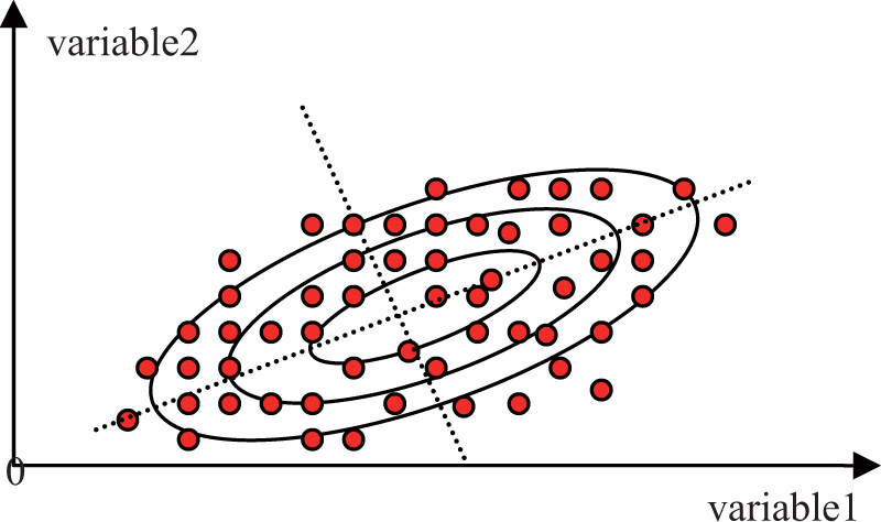
Spatial distribution by bivariate

Lemma 1

f(x)=(2π)−p/2Σ−1/2exp⁡{(x−μ)TΣ−1(x−μ)}

From the aspect of likelihood, on the assumption that a random process includes the outcomes X₁, X₂, · · · , X_n, at a random experiment, if X_i occurs, then X_i has the largest probability[21], as Lemma 2 expressed. Generally speaking, the event is determined by parameter, e.i., different parameters result to different outcomes. If one occurs, the corresponding parameter is taken as likelihood estimation. Hence, the occurrence should not be measured only by the data itself but rather by its spatial distribution.

Lemma 2

L(θ^)=maxθ⁡f(x1,x2,⋯,xn;θ)

3 Generic Voronoi Diagram

3.1 Voronoi Diagram

Definition 1

Voronoi Diagram.

Provided that P is a spatial set of points with Cartesian coordinate system, for any point l_k(l_x, l_y) in P space, if the distance l_k to the point p_i(p_x, p_y) is not greater than that l_k to the other points X under the function of Euclidean distance d, then the domain maked up by its trajectory is a ordinary Voronoi diagram of p_i, namely V(p_i), as shown below:

VVpi={p|d(lk,pi)≤d(lk,XX),j≠i,i,j∈II}

s.t.

d(lk,pi)=(px−lx)2+(py−ly)2

Voronoi diagram can be expressed by following formula V and Figure 3(a) in visualization.

Figure 3

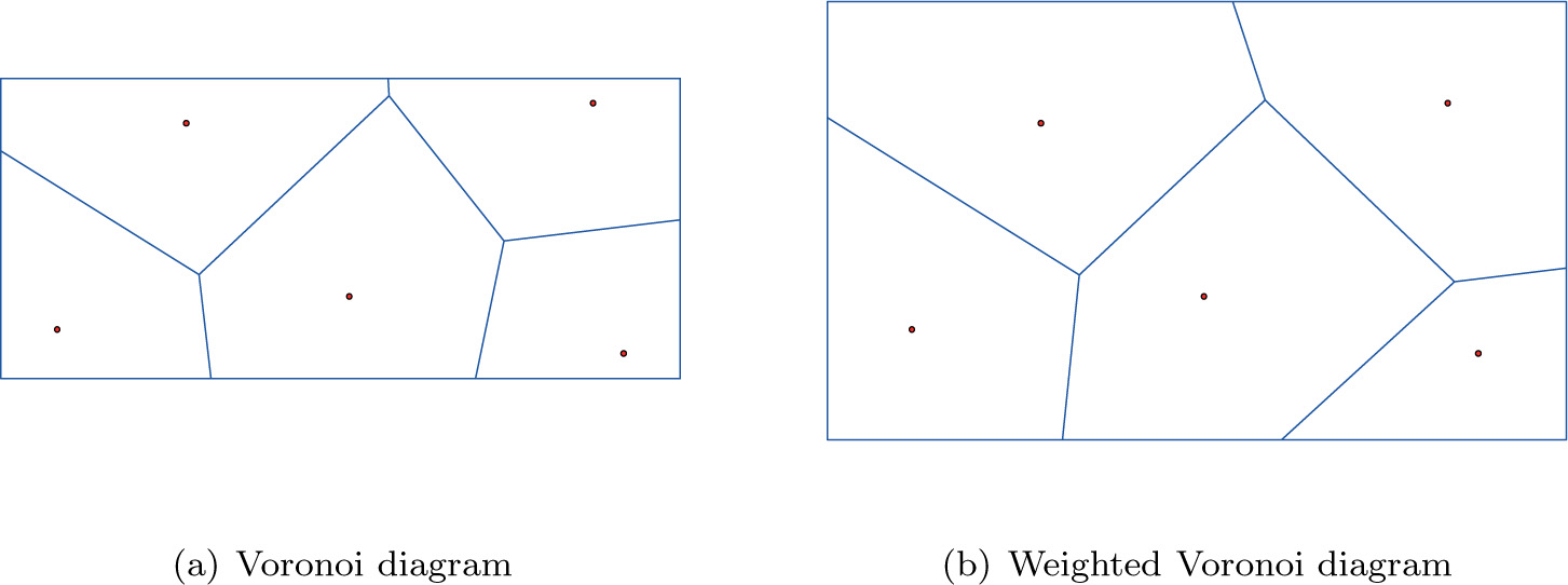
Voronoi diagram by different Euclidean distance forms

VV={VVp1,VV(p2),⋯,VVpn}

When the distance function is modified by d(l_k, p_i) – w_i, the range marked up by this weighted distance one the domain is weighted Voronoi diagram[22], as Figure 3(b) shows.

Euclidean distance is known quite well and commonly used in application, but it still has some defect and limitation, e.g., dimension closely related and without considering relativity among data. Besides, from the aspect of statistics, the component vectors in Euclidean space are not related and endowed with the same covariance, or rather, every component vector has the same contribution (weight and covariance) to distance function. Only under this condition, can it be proper in practice, or else it will not reflect actual situation faithfully. As a result, the Voronoi diagram generated by the Euclidean distance will result to erroneous or uncertain conclusions under uncertain data and distribution.

3.2 Statistical Voronoi Diagram

As Euclidean distance is inapplicable for most statistics, when the coordinates are measured by random fluctuation range, those with larger variability should be weighted more than those with less variability[23]. Consequently, the covariance and relativity need to be considered closely. In multivariate statistics, Mahalanobis distance could rule out the dimension influence obtained from spatial sampling[24], its distance function d_m is expressed as below:

dm(x,μ)=(x−μ)Σ−1(x−μ)T

In which, μ stands for mean value, and Σ stands for covariance.

Σ=σ12σ12σ21σ22

When Σ is simplified into unit matrix, the distance function is modified into Euclidean distance function, the circles in Figure 4 for instance.

Figure 4

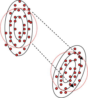
Mahalanobis distance

In practice, the mean value μ̂ and covariance Σ̂ derived from samples X̅, S, which are regarded as an unbiased estimation for global calculation respectively, as below formula shows.

μ^=X¯Σ^=Sn−1

Definition 2

Statistical Voronoi Diagram.

On the assumption that P is a spatial set of points with Cartesian coordinate system, for any point l_k(l_x, l_y) in P space, if the distance l_k to the point p_i(p_x, p_y) is not greater than that l_k to the other points X in P space under the function of Mahalanobis distance d_m, then the range maked up by its trajectory on the domain is a statistical Voronoi diagram of p_i, namely V_m(p_i).

VVmmpi={p|dm(lk,pi)≤dm(lk,XX),j≠i,i,j∈II}

The statistical Voronoi diagram can be expressed by formula V_m and Figure 5 in visualization, including Voronoi and weighted Voronoi in a wide sense.

Figure 5

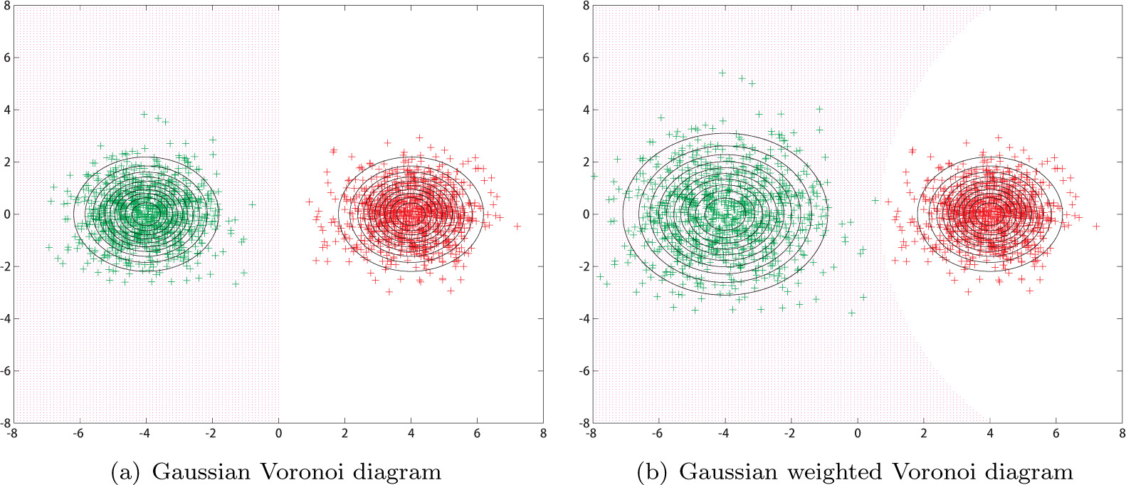
Statistical Voronoi diagram

VVmm={VVmmp1,VVmmp2,⋯,VVmmpn}

4 Empirical Results and Analyses

The samples in this experiment include different existing formulations of Voronoi diagram because of diverse covariance matrices. For example, covariance matrix of the same correlation value in the same direction, covariance matrix of different correlation values in the same direction and covariance matrix of different correlation values in different directions. The simulated analog spatial data that follows Gaussian distribution in experiment is acquired by Matlab 6.5 in this paper. The Voronoi can be produced by covariance matrix with the same correlation value in the same direction and the weighted Voronoi could be generalized by covariance matrix with different correlation values in the same direction, and the statistical Voronoi can be produced by covariance matrix with different correlation values in different directions through Mahalanobis distance function. Furthermore, the statistical Voronoi, e.i., cross Voronoi, is presented by several separated parts and expressed in a form of discreteness. Therefore, cross Voronoi diagram could extend its action range along the spatial distribution direction of the generating domain cell.

The formula 1 visualized by Figure 6 refers to the same correlation value in the same direction in covariance matrix:

Figure 6

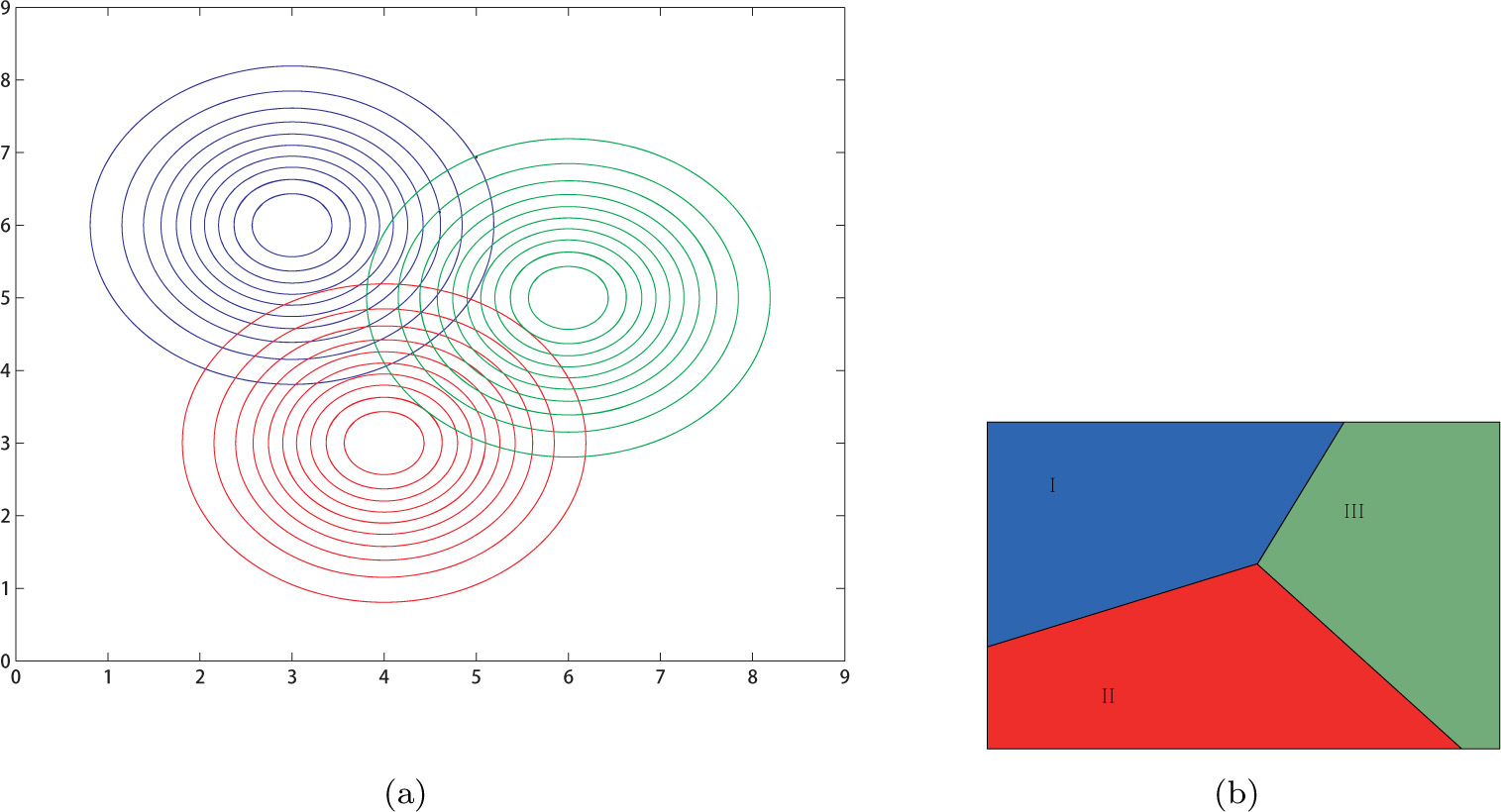
Voronoi diagram in the same covariance matrix

Formula 1

The formula 2 visualized by Figure 7 refers to the different correlation values in the same direction in covariance matrix.

Figure 7

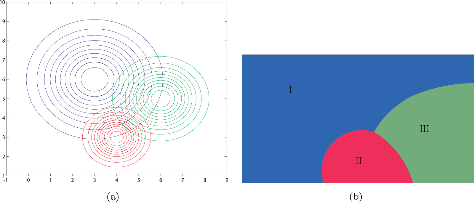
Voronoi diagram in unequal covariance matrix

Formula 2

The formula 3 visualized by Figure 8 refers to the different correlation values in different directions in covariance matrix:

Figure 8

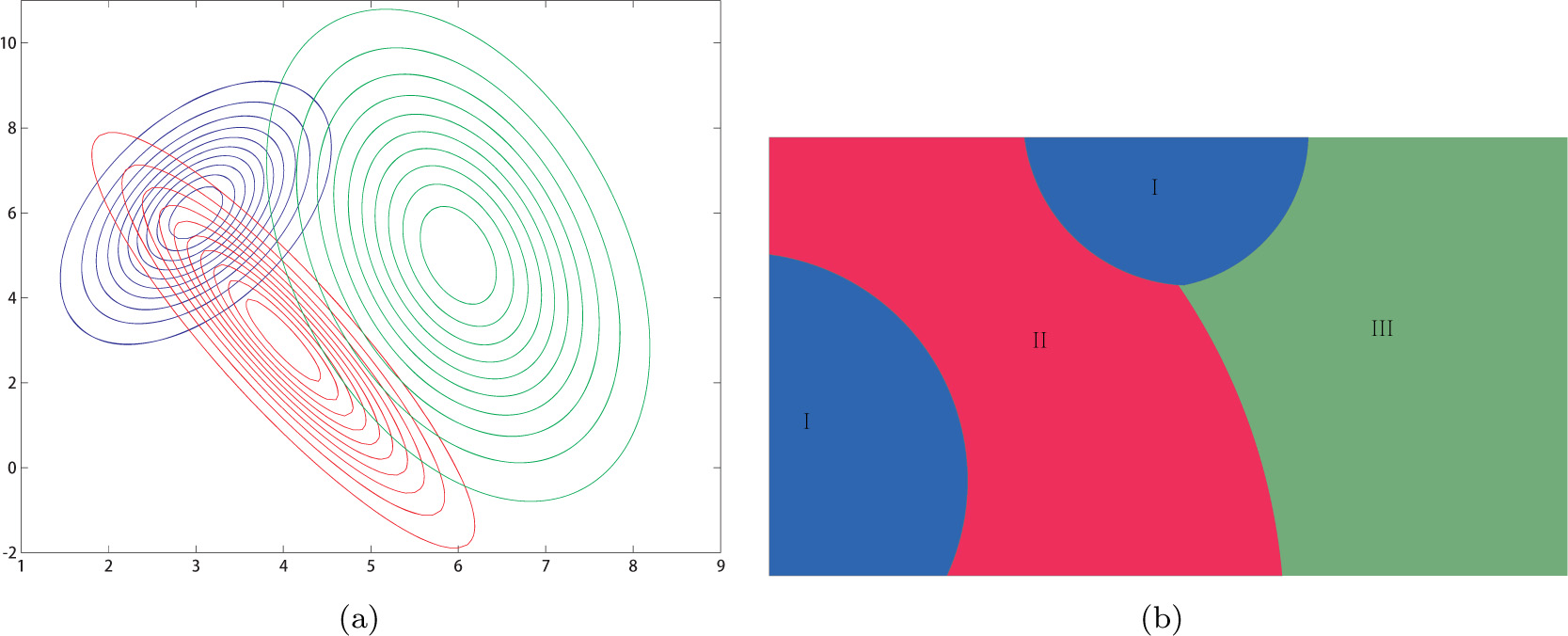
Voronoi diagram in different covariance matrix

Formula 3

Taking the existing data relativity into consideration, Voronoi diagram is produced by the same covariance matrix as Figure 6 shows. The weighted Voronoi diagram is generated with unequal covariance matrix as Figure 7 shows. So the Voronoi diagram and weighted Voronoi diagram could be generated through the definition of Mahalanobis distance, ruling out the extra weight parameter in the distance function. In addition, the cross Voronoi diagram is generated, which breaks the traditional scenario that one Voronoi diagram is merely in one range under its continuous domain. As Figure 8 shows, statistical Voronoi domain I is divided by Voronoi domain II, namely, a part of Voronoi range I crosses Voronoi domain II to extend its action range, its action range is not only a continuous part any more, but also it could be existing in two discrete forms in space.

5 Conclusions

For the limitation of traditional Voronoi and weighted Voronoi diagram, a new definition of statistical Voronoi diagram is proposed through statistical function of Mahalanobis distance and there is no need to think about the weight parameter which is determined adaptively by the spatial distribution in data itself. The definition of statistical Voronoi diagram makes the Voronoi diagram be more generalizable. Not only does it expand the theory research scope, but also produces the cross Voronoi range, redeeming the divisibility of one Voronoi domain.

In summary, the extensive definition of Voronoi diagram, namely statistical Voronoi diagram, on one hand, generalized the distance definition of Voronoi diagram and weighted Voronoi diagram; on the other hand, the produced cross Voronoi region, which was obstructed by the other Voronoi diagram in this paper, will be a certain alternative for practical applications. For the underlying effect on it, there still need further research and make efforts in this field.

References

[1] Voronoi G. Nouvelles applications des paramètres continues à la théorie des formes quadratiques. Journal für die Reine und Angewandte Mathematik, 1908, 134: 198–287.10.1515/crll.1908.134.198Suche in Google Scholar
[2] Aurenhammer F. Voronoi diagrams — A survey of a fundamental geometric data structure. ACM Computing Surveys, 1991, 23(3): 345–405.10.1145/116873.116880Suche in Google Scholar
[3] Dong P. Generating and updating multiplicatively weighted Voronoi diagrams for point, line and polygon features in GIS. Computers & Geosciences, 2008, 34(4): 411–421.10.1016/j.cageo.2007.04.005Suche in Google Scholar
[4] Aurenhammer F, Edelsbrunner H. An optimal algorithm for constructing the weighted Voronoi diagram in the plane. Pattern Recognition, 1984, 17(2): 251–257.10.1016/0031-3203(84)90064-5Suche in Google Scholar
[5] Du Q, Faber V, Gunzburger M. Centroidal Voronoi tessellations: Applications and algorithms. SIAM Review, 1999, 41(4): 637–676.10.1137/S0036144599352836Suche in Google Scholar
[6] Ju L, Du Q, Gunzburger M. Probabilistic methods for centroidal Voronoi tessellations and their parallel implementations. Parallel Computing, 2002, 28(10): 1477–1500.10.1016/S0167-8191(02)00151-5Suche in Google Scholar
[7] Boissonnat J, Nielsen F, Nock R. Bregman Voronoi diagrams. Discrete & Computational Geometry, 2010, 44(2): 281–307.10.1007/s00454-010-9256-1Suche in Google Scholar
[8] Sud A, Fisher D, Lee H. Fast dynamic Voronoi treemaps. ISVD 2010 — 7th International Symposium on Voronoi Diagrams in Science and Engineering, 2010, 85–94.10.1109/ISVD.2010.16Suche in Google Scholar
[9] Chen J. Voronoi-based dynamic spatial data model. Beijing: Publishing House of Surveying and Mapping, 2002.Suche in Google Scholar
[10] Chen J, Li C, Li Z, et al. A Voronoi-based 9-intersection model for spatial relations. International Journal of Geographical Information Science, 2001, 15(3): 201–220.10.1080/13658810151072831Suche in Google Scholar
[11] Chen J, Zhao R, Li Z. Voronoi-based k-order neighbour relations for spatial analysis. ISPRS Journal of Photogrammetry and Remote Sensing, 2004, 59(1–2): 60–72.10.1016/j.isprsjprs.2004.04.001Suche in Google Scholar
[12] Chen J, Zhao X, Li Z. An algorithm for the generation of Voronoi diagrams on the sphere based on QTM. Photogrammetric Engineering and Remote Sensing, 2003, 69(1): 79–89.10.14358/PERS.69.1.79Suche in Google Scholar
[13] Zhao R. Voronoi methods for computing spatial relations in GIS. Beijing: Publishing House of Surveying and Mapping, 2006.Suche in Google Scholar
[14] Li J, Chen J, Zhao R, et al. A backward inflation generating method for Voronoi diagram based on linear quadtree structure. Acta Geodaetica et Cartographica Sinica, 2008, 37(2): 236–242.Suche in Google Scholar
[15] Hu S, Jin L, Donguk K, et al. A sweepline algorithm for Euclidean Voronoi diagram of circles. Computer Aided Design, 2002, 38(3): 260–272.10.1016/j.cad.2005.11.001Suche in Google Scholar
[16] Ai T, Yu W. Algorithm for constructing network Voronoi diagram based on flow extension ideas. Acta Geodaetica et Cartographica Sinica, 2013, 42(5): 760–776.Suche in Google Scholar
[17] Shi W. Principles of modeling uncertainties in spatial data and spatial analyses. CRC Press, 2009: 8–12.10.1201/9781420059281Suche in Google Scholar
[18] Zhang J, Yang Y. Analysis on the status of spatial data uncertainty research. Geospatial Information, 2009, 7(3): 4–8.Suche in Google Scholar
[19] Ren X, Yu X. Multivariable statistical analysis. Beijing: China Statistics Press, 2011: 63–65.Suche in Google Scholar
[20] Li D, Wang S, Li D, et al. Theories and technologies of spatial data mining and knowledge discovery. Geomatics and Information Science of Wuhan University, 2002, 27(3): 221–233.Suche in Google Scholar
[21] Fisher R. On the mathematical foundations of theoretical statistics. Philosophical Transactions of the Royal Society, 1922, A: 222: 309–368.10.1007/978-1-4612-0919-5_2Suche in Google Scholar
[22] Balzer M, Deussen O. Voronoi treemaps. Proceedings of IEEE Symposium on Information Visualization, INFO VIS, 2005: 49–56.Suche in Google Scholar
[23] Richard A, Dean W. Applied multivariable statistical analysis. United States: Prentice Hall, 2001: 22–27.Suche in Google Scholar
[24] Mahalanobis P C. On the generalized distance in statistics. Proceedings of the National Institute of Science of India, 1936, 12: 49–55.Suche in Google Scholar
© 2015 Walter de Gruyter GmbH, Berlin/Boston
Artikel in diesem Heft
- Domino Effect Analysis, Assessment and Prevention in Process Industries
- Carbon Emissions and Carbon Intensity in China’s Exports: A Contrast of SRIO and GIRIO Methods
- Game Analysis in a Dual Channels System with Different Power Structures and Service Provision
- Uniform Parallel Machine Scheduling Problem with Controllable Delivery Times
- Dealing with Interval DEA Based on Error Propagation and Entropy: A Case Study of Energy Efficiency of Regions in China Considering Environmental Factors
- A Data-Centric Approach for Model-Based Systems Engineering
- Testing for Spatial Lag Effects in Varying Coefficient Spatial Autoregressive Models