A Dynamic Formation Procedure of Information Flow Networks
-
Hongwei Gao
 ,
Artem Sedakov
,
Artem Sedakov

Abstract
A characterization of the equilibrium of information flow networks and the dynamics of network formation are studied under the premise of local information flow. The main result of this paper is that it gives the dynamic formation procedure in the local information flow network. The research shows that core-periphery structure is the most representative equilibrium network in the case of the local information flow without information decay whatever the cost of information is homogeneous or heterogeneous. If the profits and link costs of local information flow networks with information decay are homogeneous empty network and complete network are typical equilibrium networks, which are related to the costs of linking.
1 Introduction
The main actors of an information flow network are players. The difference between the information flow network and a regular network is that the equilibrium of information flow network depends on its topological structure and players have the need and competence of acquiring information personally. The dynamic formation procedure of information flow network is one of the most worthy of concern questions[1]. In actual practice individuals decide on information acquisition and links with others over time, and it is important to understand these dynamics. Similar to “Two-way” flow network model in common sense[2], an important assumption is that “unilateral formation connection and bilateral information exchange”, that is to say, a link is formed once some player pays for it and it allows both players to access the information personally acquired by the other player.
In this paper, we study the characterization of the equilibrium of local information flow networks and the dynamics of network formation. We give the dynamic formation procedure of the local information flow network. The research shows that core-periphery structure is the most representative equilibrium network in the case of the local information flow without information decay whatever the cost of information is homogeneous or heterogeneous. If the profits and link costs of local information flow networks with information decay are homogeneous empty network and complete network are typical equilibrium networks, which are related to the costs of linking.
This work is related to a number of literatures. First, there is a theoretic literature on social networks from a game perspective[3–14]. Second, there is an extensive literature from the applying perspective[15–18].
2 Local Information Flow Networks Without Information Decay
2.1 Equilibrium Networks in the Static Case
Let N = {1, 2, ⋯, n} with n ≥ 3 be the set of players and let i and j be typical members of this set. Each player chooses a level of personal information acquisition xi ∈ X = [0, +∞) and a set of links with others to access their information, which is represented as a (row) vector:
where gii = 0, ∀i ∈ N and gij ∈ {0, 1}, for each j ∈ N\{i}. We say that player i has a link with player j if gij = 1, and the cost of linking with one other person is k > 0. Otherwise we have gij = 0. Our paper assumes that the cost of linking with one other person is homogeneous, and the link between player i and j allow both players share information. The set of strategies of player i is denoted by Si = X × Gi. Define S = S1 × S2 × ⋯ × Sn as the set of strategies of all players. A strategy profile s = (x, g) ∈ S specifies the personal information acquired by each player x = (x1, x2, ⋯, xn), and the network of relations (connection Matrix) g = (g1, g2, ⋯, gn)T, where T specifies a transposition.
The network g is a directed graph, where the arrow from i to j specifies gij = 1. Let G be the set of all possible directed graphs on n vertices. Define Ni(g) = {j ∈ N : gij = 1} as the set of players with whom i has formed a link. Let ηi(g) = | Ni(g) |. The closure of g is an undirected network denoted by g = cl(g), where gij = max{gij, gji}. In words, the closure of a directed network involves replacing every directed edge of by an undirected one. Define Ni(g) = {j ∈ N : gij = 1} as the set of players directly connected to i. The undirected link between two players reflects bilateral information exchange between them.
The payoff to player i under strategy profile s = (x, g) is
where ci > 0 is the cost of information. We assume the cost of information that personally acquired is heterogeneous. We also assume that f(y) is twice continuously differentiable, increasing, and strictly concave in y. To focus on interesting cases we assume
and
Under these assumptions, there exists a number ŷi > 0 such that
i.e., ŷi solves f′(ŷi) = ci.
A Nash equilibrium is a strategy profile s* = (x*, g*) satisfying
Example 1
Let N = {1, 2, 3, 4, 5, 6} be the set of players, the cost of linking with one other person be homogeneous k =
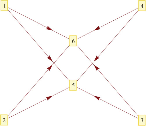
A network
Notice that equilibrium network in this example has typical “two-core-periphery” architecture. Player 5 and Player 6 become two hubs because they have slightly lower costs of acquiring information, the information that they acquire personally is
However, when spokes acquire the optimal aggregate information 1 personally and do not link with hubs, the payoff is
Similarly, we can verify Πi (s) < Πi (s*), ∀s ∈ Si, ∀i ∈ N. So the spokes form links with two hubs while do not form links between them and two hubs do not form links between them is the equilibrium strategy for the players.
In this example, there is no link between two hubs because of k > c5ŷ6 = c6ŷ5 (0.2 >
As we see in Example 1, the cost heterogeneity of information acquisition is based on two levels. The primary cause lies in the high complexity of the algorithm of general equilibrium network. In fact, slight cost difference can help us distinguish which players attain information actively and which players become spokes.
To simplify symbolic system, we mark ŷ1 and ŷ as the optimal value of information, which are obtained by players who have information cost advantage and have not advantage. We use
In the network g with core-periphery architecture, we assume that Nc(g) be the set of hubs, where | Nc(g)| = m, then N\Nc(g) be the set of spokes, and we have | N\Nc(g)| = mq, where q ∈ N+, namely n = (q + 1)m. The homogeneous cost of linking with one other person is k which satisfies f(ŷ) − c ŷ < f(mŷ1) − mk.
Lemma 1
In the equilibrium networks with core-periphery architecture, if for eachl ∈ N, we have xl > 0, then xi + yi = ŷ1, for each i ∈ Nc(g). Moreover, xp + yp = ŷ, for each p ∈ N\Nc(g).
The proof of this lemma is similar to Lemma 1 in [1].
Definition 1
The local information flow network is called core-empty-periphery, if for any pair of players i, i′ ∈ Nc(g), we have gii′ = 0, and for each player p ∈ N\Nc(g), we have gp1 = gp2 = ⋯ = gpm = 1.
Definition 2
The local information flow network is called core-completely-periphery, if for any pair of players i, i′ ∈ Nc (g), we have gii′ = 1, and for each player p ∈ N\Nc(g), we have gp1 = gp2 = ⋯ = gpm = 1.
Theorem 1
The local information flow network is a equilibrium network with “core-empty-periphery” architecture, if
the personal information acquired by each player i is
the personal information acquired by each player p is
cxp < k < cxi,
In fact, the first inequality in term 3) assures that spokes are not being connected and spokes are favorable to link with hubs; the second inequality assures that hubs are not being connected; the third inequality assures that spokes link with hubs if they acquire partial information actively. Meeting with information level of terms 1) and 2) can guarantee hubs owning the aggregate information ŷ1 in the network, while the aggregate information owned by spokes is ŷ. It is shown in Example 1.
Theorem 2
The local information flow network is a equilibrium network with “core-completely-periphery” architecture, if
The personal information acquired by each player i is
The personal information acquired by each player p is
Similar to Theorem 1, the first inequality in term 3) assures that spokes do not form links between them while hubs are favorable to form links with each other and spokes are favorable to form links with hubs; the second inequality assures that spokes link with hubs if they acquire partial information actively. Meeting with information level of terms 1) and 2) can guarantee hubs own the aggregate information ŷ1 in the network, while the aggregate information owned by spokes is ŷ.
We can see from the above situation, after fixing the amount of hubs, the information acquisition of spokes is degressive. So if q ⟶ + ∞, then xp ⟶ 0. Relatively, the information acquisition of hubs is increasing.
The result also reflects contents of “The law of the few”, that is a lot of information will be grasped in a few hubs, while most of other players, that is, the spokes will choose to link with hubs to get information, but themselves will choose little “personal information acquisition”, or even entirely depends on the connection to get information, making their “personal information acquisition” to zero.
Example 2
Let N = {1, 2, 3, 4, 5, 6, 7, 8, 9} be the set of players, the cost of linking with one other person be homogeneous, we denote by k = 0.15, the cost of information that personally acquired be heterogeneous and is denoted by c1 = c2 = c3 = c4 = c5 = c6 =
We can check that s* = (x*, g*) is a Nash equilibrium, where
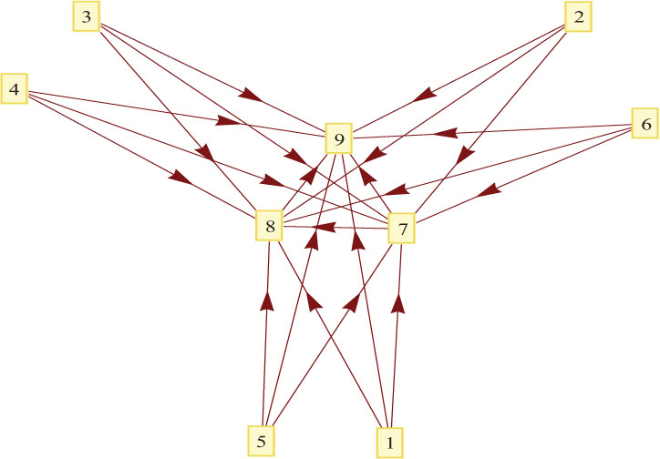
A three-core-completely-periphery equilibrium network
2.2 A Dynamic Formation Procedure and the Algorithm
The algorithm of finding equilibrium networks in this paper is based on a dynamic procedure used in [12, 19, 20].
Given the set of players, at each stage, agents who are chosen at random play their best response, adjust their links in response to the network structure and the personal information acquired by oneself in previous period and then compose the network structure and the personal information (it is called the player’s non-coordinated behavior).
At stage t, first select a subset R of the set of players N at random. For every selected player i ∈ R, we calculate his optimal personal information and the best link set by comparing all of his possible links, namely the player’s best response strategy. Each player who is selected at random chooses a pure strategy best response to the strategy of all other agents in the previous period and for the player who is not selected he maintains the strategy chosen in the previous period. Compose all strategies, and then dynamic procedure comes to stage t + 1.
Based on above dynamic procedure, the advantage of the algorithm is that the optimization question has only one variable. The network reaches a stable state when no one chooses to change his links and personal information during dynamic procedure, and then we can get equilibrium strategy profile s* = (x*, g*) and relative information equilibrium network.
Given an initial stage t0, an initial information vector
At stage t, let information vector be
Select randomly the set of players R = (i1, i2, ⋯, ir) ⊆ N. For every ik ∈ R, the row ik of link matrix has 2n−1 possibilities if we fix the rest n − 1 rows. For every possibility, first calculate
Consider that
subject to
Notice that
Suppose that the optimal value is reached at
Let
be link matrix at stage t + 1, and information vector
The dynamic procedure comes into stage t + 1. Select the set of players at random again and the network formation procedure is repeated.
The dynamic procedure is end until no one chooses to change his links and personal information. At last we get the information flow equilibrium network and equilibrium strategy profile will comprise the link matrix of the equilibrium network and the optimal personal acquired information vector. It should be noticed that to guarantee the valid of the algorithm we must suppose that the dynamic procedure is not a circulation.
Example 3
Given the set of players N = {1, 2, 3, 4, 5, 6}, homogeneous link costs k = 0.04 and personal information heterogeneity costs c1 = c2 = c3 = c4 =
It is different to reach final stage for each implementation of the dynamic process program and convergence to the equilibrium state because the non-coordinated behavior of the players caused by the randomness of process of forming network. Therefore there is not practical significance for number of stages to achieve an equilibrium state.
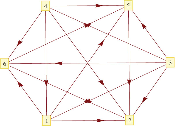
We only had one interception of several typical stages in some run results in Figure 3, and let K be the number of stages needed to achieve an equilibrium state.
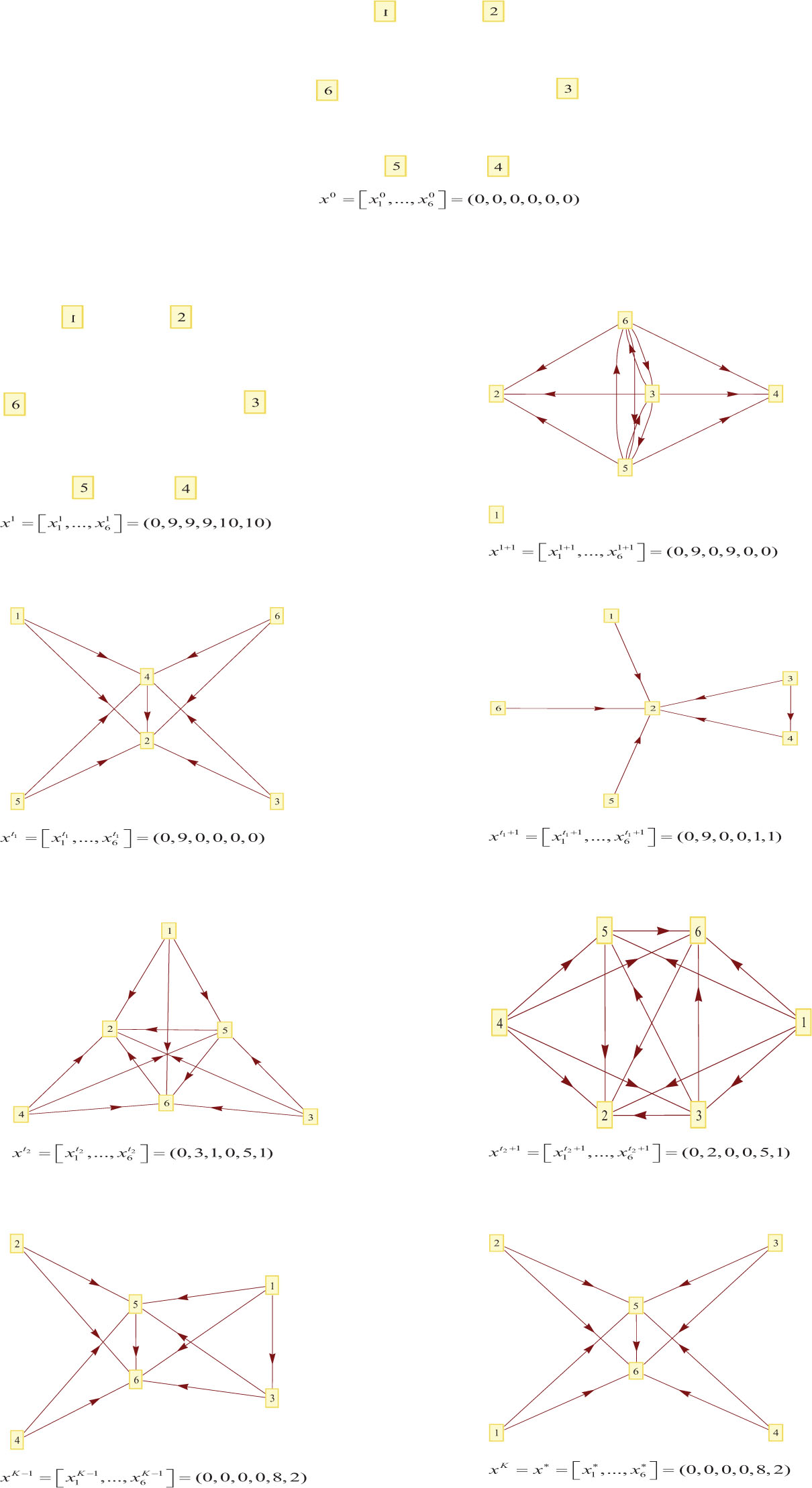
Stage example of the dynamic process
The network structure and dynamics of information vectors in Example 3:
At the initial stage we select the set of players R = {2, 3, 4, 5, 6} at random, because of the initial matrix is zero, they all choose to acquire their optimal aggregate information and do not form any link. And then it will come into an empty network by the first round of iteration. But the information level vector is
If the selected set of players is R = {3, 5, 6} at stage 1, we can infer that it is the best response for Player 3 to form links with Players 2, 4, 5 and 6 and he do not acquire information personally, the payoff Π3(.) = ln[1 + (9 + 9 + 10 + 10)] − 4 × 0.04 ≈ 3.5036 is larger than the payoff in any other situation. Because Players 5 and 6 have the same acquired advantage, it is the best response for Players 5 and 6 to form links with 2, 3, 4, 6 and he do not acquire information. The dynamic procedure comes into stage 2.
When the dynamic procedure comes into stage t1, the current network has two-core-periphery architecture. The information level vector of players is xt1 = (0, 9, 0, 0, 0, 0). Select set of the players R = {1, 4, 5, 6} randomly. Although here the two-core-periphery architecture is the same as the eventual equilibrium structure formally (Players 2 and 4 are temporal core), obviously, for Players 5 and 6 their aggregate information do not reach their optimal value ŷ5 = ŷ6 = 10, so here the network is not an equilibrium network and not stable. For Players 5 and 6 they will delete their links with Player 4 and maintain their link with Player 2 and acquire information 1 by themselves, the payoff Πi(⋅) = ln[1 + (9 + 1)] −
When the dynamic procedure comes into stage t2, the current network has three-core-completely-periphery architecture. The information level of players is xt2 = (0, 3, 1, 0, 5, 1). Selected set of the players R = N. So here for Players 1 and 4 it is their best response to maintain their links with Players 2, 3, 5 and 6. Players 2 and 3 will maintain their links and reduce their information 1 by themselves and for Players 5 and 6 they maintain their strategies from the previous period. Notice that here the network is four-core-completely-periphery architecture, it is not stable.
When the dynamic procedure comes into stage K − 1, the information level of players is xK−1 = (0, 0, 0, 0, 8, 2). Selected set of the players R = {1} randomly. For Player 1 his best response is to delete his link with Player 3 and maintain his link with 5 and 6 while he acquires no information. The “two-core-periphery” equilibrium network is formed. The hub is composed of two players with information cost advantage acquired actively. The dynamic procedure is over.
Core-periphery structure is the most representative equilibrium network in the case of the local information flow without information loss. In fact, under the premise of players have two levels of information each person who has a comparative advantage of the cost of acquiring information would become the hub possibly. The statistical results show that it is the easiest to form “single-core-periphery” structure; but the “multi-core-periphery” structure which contains all players who has the same advantage on the cost as the hubs (maximum) has the smallest probability; those which between these two kinds become harder and harder with the increasing of the players’ number in the core.
We believe that there are several reasons why the dynamics are important. One of the reasons is that a dynamic model allows us to study the process by which individual agents learn about the network and adjust their links in response to their learning. And the dynamics may help select among different equilibria of the static game.
There is very important prospect to study the characterization of the architecture of information flow equilibrium networks and the dynamics of network formation under the premise of local information flow and without the presence of decay. In addition, consider that some of the players may coordinate and prepare to maximize the common interests of members by some local cooperation; the model and algorithm in this essay can be transformed to an incomplete information cooperative game model. This article assumes that the players have the need and competence of acquiring information personally and getting information from others in the given network structure, in fact, this can also be diversified.
3 Local Information Flow Networks with Information Decay
Lemma 2
In the local information flow equilibrium network g with information decay, we have xi + yi ≥ ŷ, for all i ∈ N, and ifxi > 0, thenxi + yi = ŷ. Hereyi = ∑j ∈ Ni(g)δ xj, that is to say yi represents the information that Player i acquires from his neighbors.
Proof
Suppose not, then there must exist some Player i such that xi + yi < ŷ in equilibrium network g. Under the assumptions that f(y) is twice continuously differentiable, increasing, and strictly concave in y, we know f′(xi + yi) > c, so Player i can strictly increase his payoffs by increasing personal information acquisition, a contradiction with equilibrium. So we know xi + yi ≤ ŷ, ∀ i ∈ N. Next suppose that xi > 0 and xi + yi > ŷ. Under our assumptions on f(⋅) and c, if xi + yi > ŷ then f ′(xi + yi) < c, and then Player i can strictly increase his payoffs by lowering personal information acquisition, which contradicts equilibrium. Therefore, if xi > 0, then xi + yi = ŷ.
Theorem 3
In the local information flow equilibrium network with information decay, if k > cδŷ, the empty network is unique equilibrium. Every player acquires information ŷ personally and no one forms links.
Proof
Suppose that the strategy profile s = (x, g) corresponds to an empty network. If Player i forms m1 links with other m1 players and personally acquires information
however, in the empty networks, his payoff is
Since k > cδŷ, we have
Suppose Player i forms m2 links with other m2 players initiatively based on the empty network, and
Here δm2ŷ ≥ ŷ, then δm2≥ 1. Therefore
Due to k > cδŷ, the first inequality is strict obviously, since f(y) is twice continuously differentiable, increasing, and strictly concave in y, the second is hold. Then the empty network is an equilibrium network.
Finally, we will show that the empty network is the unique equilibrium. As we know, every player’s personal information acquisition is no more than ŷ, if some Player i wants to form a link with other player (say j), Player i can obtain δxj from j, and cδxj > k, this would contradict with k > cδŷ (because ŷ > xj).
Lemma 3
If complete network is the local information flow equilibrium network with information decay, the personal information acquisition of each player equals
Proof
For every player he acquires information personal xi ≥ 0. If there are m(1 ≤ m < n) players who personally acquires information 0, we let x1 = x2 = ⋯ = xm = 0, according to Lemma 2, we conclude following inequalities:
We can obtain xm+1 = ⋯ =
therefore
Theorem 4
In the local information flow equilibrium network with information decay, if
Proof
Firstly prove that if the personal information acquisition of each player equals x =
Secondly, we show that it is not the best response for Player i of deleting links or changing his personal information level.
Now consider the case m = 0, Player i can change their personal information acquisition to be x′, we can write strategy profile s*|
so changing strategies is not the best response for Player i.
Consider the case m = 1, if Player i deletes links and acquires information (1 + δ)x personally, hence
Since k < cδx,
so changing strategies is not the best response for Player i.
Similarly, we can show that the best response for Player i is to maintain current strategy and completeness of network when m = 2, 3, ⋯, n − 1 and k < cδx.
In the following we show that if
Lemma 3 implies that if a complete network is the equilibrium structure, the personal information acquisition of each player equals
Two steps: The first step is to prove the connected but not completely network is not equilibrium, the second step is to prove not connected network is not the equilibrium.
Step 1:
Suppose the connected but not completely network is an equilibrium. Noticed that the equilibrium network must be essential[2].
We delete any link in complete network, gij = 0 or gji = 0, let g1 be the network. Suppose g1 is equilibrium. By Lemma 2, every player’s aggregate information should be more than or equal to ŷ. Since gij = 0, we have k > cδxi and k > cδxj. Players who are in N {i, j} have links with each other, let N1 = {i, j}, N2 = N{i, j}, I(s) = {p|xp > 0, p ∈ N}. For q ∈ N2∩ I(s), we have
If xi = xj = 0, and i, j ∈ N1, so that
a contradiction with equilibrium.
If xi = 0, xj > 0, and i ∈ N1, hence
then Player i can strictly increase his payoffs by increasing personal information acquisition. It contradicts with equilibrium.
The case of xj = 0, xi > 0 is similar to the above.
Hence, we can conclude that personal information acquisition of i and j more than 0. Otherwise, for l ∈ N2\ I(s), we have
That is to say, the aggregate information of l is less than ŷ, contradiction. Hence, for any i ∈ N, every player’s personal information acquisition is xi > 0. According to Lemma 2, the following inequalities are held
So the personal information acquisition in N1 equals to xi = xj = x′, and the personal information acquisition in N2 equals to xq = x″, ∀ q ∈ N2, so that
For any n ≥ 3, any network is not equilibrium network.
Similarly, we can show that except complete network, connected network is not the equilibrium network.
Step 2:
Firstly, suppose there is an isolated player in equilibrium network at least, the set of these players is N0. The personal information acquisition is ŷ in N0. Due to k < cδx < cδŷ, there must exist some player in N \ N0 who will strictly increase his payoffs by lowering his personal information acquisition and switching to link with players in N0, contradiction with equilibrium.
Secondly, suppose C1(g) and C2(g) are two parts of the network g, and every part has more than one player.
From Step 1, we know that the two parts are complete.
Suppose | C1(g)| = n1 > 1, | C2(g)| = n2 > 1, and assume n1 ≤ n2. Lemma 2 and Lemma 3 claimed that the information is equal in C1(g) and C2(g), respectively:
Then xn1 ≥ xn2 > x. We can concluded that k < cδx < cδxn2 ≤ cδxn1, the players in C2(g) will link with the players in C1(g) initiatively. A contradiction completes the proof.
Similarly, we can show that non-connected network which contains multiple parts is not the equilibrium.
Example 4
Let N = {1, 2, 3, 4, 5, 6} be the set of players, the homogeneous cost of linking with one other person is denoted by k, the homogeneous cost of information that players acquire is denoted by c, the index of local information decay is denoted by δ and 0 < δ < 1, where payoffs are given by (1), f(y) = ln(1 + y).
As shown in Figure 4, δ is x-coordinate, k is y-coordinate, where n = 6, c =
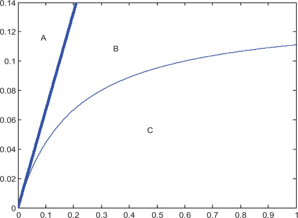
A distribution of equilibrium networks
A complete network
But if cδx < k < cδŷ,
References
[1] Galeotti A, Goyal S. The law of the few. American Economic Review, 2010, 100(4): 1468–1492.10.1257/aer.100.4.1468Search in Google Scholar
[2] Bala V, Goyal S. A noncooperative model of network formation. Econometrica, 2000, 68: 1181–1229.10.1007/978-3-540-24790-6_7Search in Google Scholar
[3] Bala V, Goyal S. A strategic analysis of network reliability. Review of Economic Design, 2000, 5: 205–228.10.1007/978-3-540-24790-6_14Search in Google Scholar
[4] Barabasi A. Linked. Perseus Books Group: New York, 2002.Search in Google Scholar
[5] Bloch F, Jackson M O. The formation of networks with transfers among players. Journal of Economic Theory, 2007, 133: 83–110.10.1016/j.jet.2005.10.003Search in Google Scholar
[6] Galeotti A, Goyal S, Kamphorst J. Network formation with heterogenous players. Games and Economic Behavior, 2006, 54: 353–372.10.1016/j.geb.2005.02.003Search in Google Scholar
[7] Galeotti A. One-way flow networks: The role of heterogeneity. Economic Theory, 2006, 29(1): 163–179.10.1007/s00199-005-0015-0Search in Google Scholar
[8] Goyal S, Vega-Redondo F. Network formation and social coordination. Games and Economic Behavior, 2005, 50(2): 178–207.10.1016/j.geb.2004.01.005Search in Google Scholar
[9] Goyal S. Connections: An introduction to the economics of networks. Princeton, Princeton University Press, 2007.10.1515/9781400829163Search in Google Scholar
[10] Goyal S. Learning in networks. Benhabib J, Bisin A, Jackson M O (eds). Handbook of Social Economics, 2011, 1: 679–727.10.1016/B978-0-444-53187-2.00015-2Search in Google Scholar
[11] Haller H, Sarangi S. Nash networks with heterogeneous links. Mathematical Social Sciences, 2005, 50(2): 181–201.10.1016/j.mathsocsci.2005.02.003Search in Google Scholar
[12] Hojman D, Szeidl A. Core and periphery in networks. Journal of Economic Theory, 2008, 139: 295–309.10.1016/j.jet.2007.07.007Search in Google Scholar
[13] Jackson M O, Wolinsky A. A strategic model of social and economic networks. Journal of Economic Theory, 1996, 71(1): 44–74.10.1007/978-3-540-24790-6_3Search in Google Scholar
[14] Jackson M O. Social and economic networks. Princeton, Princeton University Press, 2008.10.1515/9781400833993Search in Google Scholar
[15] Che X, Bu H, Liu J J. A theoretical analysis of financial agglomeration in China based on information asymmetry. Journal of Systems Science and Information, 2014, 2(2): 111–129.10.1515/JSSI-2014-0111Search in Google Scholar
[16] Yang Y, Lu X, Qiao H. A robust factor analysis model for dichotomous data. Journal of Systems Science and Information, 2014, 2(5): 437–450.10.1515/JSSI-2014-0437Search in Google Scholar
[17] Xie H B, Bian J Z, Wang M X, Qiao H. Is technical analysis informative in UK stock market? Evidence from decomposition-based vector autoregressive (DVAR) model. Journal of Systems Science and Complexity, 2014, 27(1): 144–156.10.1007/s11424-014-3280-9Search in Google Scholar
[18] Zhao Y X, Hu Z H, Qiao H, Wang S Y, Uria L C. Characterizations of semi-prequasi-invesity. Journal of Systems Science and Complexity, 2014, 27(5): 1008–1026.10.1007/s11424-014-1109-1Search in Google Scholar
[19] Gao H W, Yang H J, Wang G X, et al. The existence theorem of absolute equilibrium about games on connected graph with state payoff vector. Science China Math, 2010, 53(6): 1483–1490.10.1007/s11425-010-3075-ySearch in Google Scholar
[20] Gao H W, Petrosyan L A. Dynamics cooperative games. Beijing, Science Press, 2009.Search in Google Scholar
© 2015 Walter de Gruyter GmbH, Berlin/Boston
Articles in the same Issue
- A Dynamic Formation Procedure of Information Flow Networks
- A Study on the Optimal Portfolio Strategies Under Inflation
- A Dynamic Model of Procurement Risk Element Transmission in Construction Projects
- Can Scientific and Technological Talent Aggregation Accelerate Economic Growth? An Empirical Study
- Composite Stackelberg Strategy for Singularly Perturbed Bilinear Quadratic Systems
- Bearing Fault Diagnosis Using Orthogonal Matching Pursuit with Pulse Atoms Based on Vibration Model
- Dynamics of a Nonlinear Business Cycle Model Under Poisson White Noise Excitation
- The GM(1,1) Model Optimized by Using Translation Transformation Method and Its Application of Rural Residents’ Consumption in China