Preemptive Scheduling with Controllable Processing Times on Parallel Machines

Algorithm

A₁forPm|pmtn,pj=pj¯−xj,∑xj≤X^|Cmax

Step 1 Let x = 0. Sort all jobs in non-increasing order of basic processing time, i.e., p1¯≥p2¯≥⋯≥pn¯.

Step 2 Ifmaxj=1npj¯≤∑j=1npj¯/m, then schedule all jobs by McNaughton’s wrap-around rule. Go to Step 4.

Step 3 Schedule the longest job on one machine and delete the job. Decrement m by 1. If the longest job is the last job, then go to Step 4, else go to Step 2.

Step 4 Use all of the resource X^ to shorten the C_max backward.

See Figure 1, for the situation that all the jobs arrive at the same time, the Step 1 of Algorithm A₁ is to obtain a solution for the corresponding problem with x = 0 by using the Modified McNaughton’s rule, and get the makespan is C_max(s¹,0). The second step is to shorten the makespan backward by using the extra resources and obtain the makespan C_max(s, x).

Figure 1

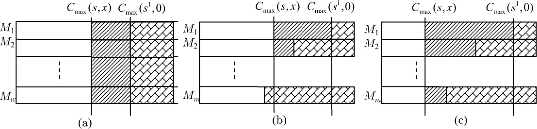
Three cases of the situation with the same release time

Theorem 1

ForPm|pmtn,pj=pj¯−xj,∑xj≤X^|Cmax, A₁ is optimal.

Proof

To prove the algorithm A₁ is optimal for the problem Pm|pmtn,pj=pj¯−xj,∑xj≤X^|Cmax, we show the following two results: (i) Let the resource allocation scheme is x in algorithm A₁, then under this resource allocation scheme, the solution (s,x) obtained by A₁ is optimal; (ii) If there is another resource allocation scheme x*, which is different to x, then we can not find another solution (s*,x*) such that C_max(s*, x*) < C_max(s, x).

(i) Let the schedule s¹ be obtained in Step 1, then s¹ is optimal for the corresponding problem P_m|pmtn|C_max according to Hong & Leung^[2]. Case 1. s¹ is a block schedule. Then it is apparent that there is no another resource allocation scheme can shorten the C_max less than C_max(s, x). See Figure 1(a). Case 2. All s¹ and s are not block. See Figure 1(b). Let the machine M_k is the first machine on which the maximal completion time equals to Cmaxmin in solution (s¹,0). The schedule s¹ is not a block schedule, so the machine M₁ to machine M_k-1 must process only one of the k – 1 longest jobs, s is not block, thus the total resources do not shorten the C_max down to Cmaxmin, and only the jobs on machine M₁ to M_k-1 are compressed. Thus the schedule (s, x) is still followed by the Modified McNaughton’s Rule. Case 3. s¹ is not block but s is not the case. See Figure 1(c). Because we shorten the C_max in Step 2 and the direction is backward, it is easy to prove that it is true by Case 2 and Case 1. So under the resource allocation scheme x, the solution (s,x) is optimal.

(ii) (s, x) is optimal under the resource allocation x, so if there is another optimal solution (s*,x*), and C_max(s*,x*) <C_max(s,x), it is not doubt that x* ≠ x. Because (s*, x*) is optimal, it must be ∑j=1nxj∗=X^. Thus ∑j=1nxj∗=∑j=1nxj. Because x* ≠ x, we can assume that there are two jobs J_p and Jq,xp>xp∗ while xq<xq∗,xp+xq=xp∗+xq∗. Let p′ and q′ be the machine number which process job J_p and J_q in the solution (s,x). Let the machine M_k is the first machine on which the maximal completion time equals to Cmaxmin in the solution (s, x). We show that when x changes to x*, there is no a schedule s* makes that C_max(s*,x*) < C_max(s,x). Casel. k = 1. The (s,x) is block, therefore there is no another resource allocation scheme x* can satisfy C_max(s*,x*) < C_max(s,x). Case 2. k ≥ 2,p′ ≥ k. This case is impossible because the corresponding x_p equals to zero, and thus it can not be reduced. Case 3. k ≥ 2, q′ = p′ < k. So C_max(s*,x*) = C_max(s,x). Case 4. k ≥ 2,p′ < k < q′. In this case, Cmaxq′=Cmaxmin, so increasing resource to reduce Cmaxq′ is nonsensical. Case 5. k ≥ 2,p′ < q′ < k. In this case, Cmaxp′>Cmaxq′. Decreasing x_p to xp∗ means to increase Cmaxp′, so it must be C_max(s*,x*) ≥ C_max(s,x). Case 6. k ≥2, q′ < p′ < k. In this case, Cmaxp′≤Cmaxq′. If Cmaxp′=Cmaxq′, then C_max(s*, x*) = C_max(s, x). If Cmaxp′<Cmaxq′, then x_p = 0 and it can not be reduced again. The situation that the number of different jobs is more than two in the two allocation schemes can be deduced according to the two jobs situation. Because the jobs are preemptive, than we can construct some pairs like above p′ and q′ by splitting some jobs, and then prove according to the above process with only two jobs with different resource allocation.

Therefore, there is no another resource allocation scheme x* and its corresponding schedule s* such that C_max(s*,x*) < C_max(s,x).

Algorithm

A₂for Modes 1 and 2 ofPm|rj,pmtn,pj=pj¯−xj,∑xj≤X^|Cmax.

Step 1 At each preemptive time (there is a job is finished or a new batch of jobs arrive), do

1. Let x = 0. Sort all the unfinished jobs or job pieces in non-increasing order of basic processing time. Let the number of the unfinished jobs or job pieces is n.

2. If maxj=1npj¯≤∑j=1npj¯/m, then schedule all jobs by McNaughton’s wrap-around rule.

3. Schedule the longest job on one machine and delete the job. Decrement m by 1. Go to 2).

Step 2 Use all of the resource X^ to shorten the C_max backward.

Theorem 2

For Modes 1 and 2 of the problemPm|rj,pmtn,pj=pj¯−xj,∑xj≤X^|Cmax, A₂ is optimal.

Proof

Let x and s be the resource allocation and sequencing schemes according to algorithm A₂ for the problem Pm|rj,pmtn,pj=pj¯−xj,∑xj≤X^|Cmax respectively. Supposing (s*,x*) is another solution, which is different from (s,x), and C_max(s*, x*) < C_max(s,x).

If there is no job, which is released in one of the some front stages, is compressed in the last stage of the solution (s*,x*), then (s*,x*) must be the same with (s,x) according to Theorem 1. So we assume that there is a job J_j is not released in the last stage and it is compressed in one of the front stages in (s*,x*), and show that it can not be optimal. Let pj∗ be the real processing time of the job J_j in (s*,x*), so xj∗=pj¯−pj∗.

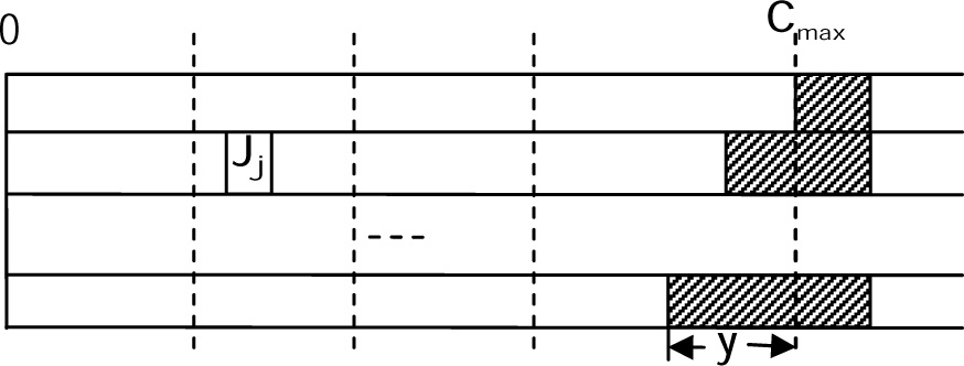
Case 1. There are some idle times before the last stage in (s*,x*). See Figure 2. If the solution (s*,x*) likes Figure 2(a), then if we allocate xj=xj∗−min(x∗,y) and assign the resource min(x*,y) to shorten the maximal completion time in the last stage, there must be another solution (s,x) is better than (s*,x*). If the solution (s*,x*) likes Figure 2(b), it is the same with Figure 2(a) except that xj=xj∗−min(x∗,z).

Figure 2

Case 1 of Theorem 2

Case 2. There is no idle time before the last stage and (s*,x*) is not block. See Figure 3. Let the machine k(k ≥ 2) is the first machine on which the maximal completion time equals to Cmaxmin in solution (s*, x*). If we reallocate xj=xj∗−min(x∗,y−ε) resources to J_j, where ε is a very little positive number. Then we can break the job J_j to two parts, the processing times of these two parts are pj∗=pj¯−xj∗ andpj′=min(x∗,y−ε) and p′_j = min(x*, y – ε). Thus we can reallocate the resources with amount min(x*, y — ε) to compress the jobs in the last stage on the k –1machines, which the maximal completion times equal to C_max. Therefore, another better solution (s,x) can be rebuilt from (s*,x*) and Cmax(s∗,x∗)−Cmax(s,x)≥min(ε,min(x∗,y−εk−1).

Figure 3

Case 2 of Theorem 2

Case 3. There is no idle time before the last stage and (s*,x*) is block. See Figure 4. In this case, if we release the resources xj∗ from the job J_j, assume that the job J_j is processed on machine M_i, thus Cmaxi=Cmax+xj∗. Then we can reallocate the resources xj∗ to shorten Cmaxi to C_max backward and the solution is still feasible. So all the solutions in this case can be transformed to the case that total resources are assigned to the jobs backward and C_max is not increased. It is easy to show that under the resource allocation backward model, the solution (s,x) satisfies the Modified McNaughton’s Rule, and thus C_max(s,x) ≤ C_max(s*, x*).

Therefore, Algorithm A₂ is optimal for the problem Pm|rj,pmtn,pj=pj¯−xj,∑xj≤X^|Cmax when total resources are released at time zero or the resources can be used in the next stages.

Figure 4

Case 3 of Theorem 2

Though Algorithm A₂ is optimal for Mode 1 and Mode 2 of the problem Pm|rj,pmtn,pj=pj¯−xj,∑xj≤X^|Cmax, it can not obtain a optimal solution for Mode 3, see Example 1.

Example 1

There are 3 machines. At time 0, the available resource amount is 1, i.e., X^0=1, and three jobs J₁, J₂ and J₃ arrive with the basic processing times as 3, 3, 2. At time 2, X^2=2, and four jobs J₄, J₅, J₆ and J₇ come with the basic processing times as 5, 3, 2, 2.

Then the solution obtained by A₂ is like Figure 5(a) and C_max = 6(X^2=2 is used to shorten J₄, J₆, and J₂). But the optimal solution is like Figure 5(b) and Cmax∗=513(X^0=1 is used to shorten J₁; X^2=2 is to shorten J₄, J₆, and J₇). The resources released at the front stages can not be used in the next stages, thus if we use the resources backward to shorten some pieces of the jobs released in the front stages, it must deteriorate the quality of the solution. Therefore for the Mode 3, we must allocate the available resources to the jobs in the current stage but not in the last stage.

Figure 5

Example 1

Algorithm A₃

At each stage at time t (a new batch jobs arrive), do

1. Let x = 0. Sort all the unfinished jobs or job pieces in non-increasing order of basic processing time. Let the number of the unfinished jobs or job pieces is n.

2. If maxj=1npj¯≤∑j=1npj¯/m, then schedule all jobs by McNaughton’s wrap-around rule. Go to 4).

3. Schedule the longest job on one machine and delete the job. Decrement m by 1. If the longest job is the last job, then go to 4), else go to 2).

4. Use the available resources X^t to compress the processing time of the jobs in the current stage backward until all the resources X^t are allocated or the maximal completion time of the current stage equals to the start time of the next stage.

Theorem 3

For Mode 3 of the problemPm|rj,pmtn,pj=pj¯−xj,∑xj≤X^|Cmax, algorithm A₃ is optimal.

This theorem is simple to prove. Because in Mode 3 of the problem with different release times, the extra resources can only be used in the current stage but not in the successive stages, we must use the available resources to shorten the maximal completion times in the current stages. But when the maximal completion time of the current stage is shortened before the start time of the next stage, it is not useful to compress the jobs any more, and then we can stop to allocate the resources in the current stage. In each stage, the method in Algorithm A₃, is optimal according to Theorem 1.

Theorem 4

There is no optimal algorithm for Modes 1 and 2 of the online version of the problemPm|rj,pmtn,pj=pj¯−xj,∑xj≤X^|Cmax.

Proof

We prove that the theorem is true for m = 2; it is easy to see that the proof can be generalized to m > 2. Suppose there is an optimal online scheduler for 2 machines and consider the following scenario. At time 0, X^0=1.J0={J1,J2}, in which the basic processing times are 1, 2 respectively. In the online version, we do not know the information about the job release dates and the available resource in the future, so it is amphibolous to use the available resource in the current stage or not. Case 1: The resource X^0=1 is used in the first stage. In this case, the maximal completion time in the first stage can controllable to 1. Now, consider the scenario where J¹ = {J₃, J₄} with basic processing times 1 and 4 are released at time 1, and X^1=0. Clearly, the makespan of the schedule that constructed by the optimal online scheduler is at least 5. However, the optimal offline makespan according to algorithm A₂ is 4. Case 2: The resource X^0=1 is not used in the first stage. In this case, the maximal completion time in the first stage is 2. However, if there is no job released again, the extra resource would not be used to compress the jobs. It is clear that the schedule is not optimal. The extra resource can not also be determined to use partly in the first stage according to Case 1 and Case 2.

As a result of Theorem 4, we are motivated to construct online scheduling algorithm for Mode 3 of the online version of the problem Pm|rj,pmtn,pj=pj¯−xj,∑xj≤X^|Cmax.

Algorithm A₄

Whenever a new batch of jobs arrive at t, do

1. Unite the unfinished jobs with the remainder compressed parts to the new batch jobs.

2. Let x = 0. Sort all the new batch jobs in non-increasing order of basic processing time. Let the number of the new batch is n.

3. If maxj=1npj¯≤∑j=1npj¯/m, then schedule all jobs by McNaughton’s wrap-around rule. Go to 5).

4. Schedule the longest job on one machine and delete the job. Decrement m by 1. If the longest job is the last job, then go to 5), else go to 3).

5. Use all available resources X^t to shorten the maximal completion time of the current stage backward.

Theorem 5

Algorithm A₄ is optimal for Mode 3 of the online version of the problemPm|rj,pmtn,pj=pj¯−xj,∑xj≤X^|Cmax.

It is clear true optimal for this situation according to Theorem 3 though the extra resource maybe is wasted.

References

[1] McNaughton R. Scheduling with deadlines and loss functions. Management Science, 1959, 6: 1–12.10.1287/mnsc.6.1.1Search in Google Scholar
[2] Hong K S, Leung J Y T. On-line scheduling of real-time tasks. IEEE Transactions on Computers, 1992, 41(10): 1326-1331.10.1109/REAL.1988.51119Search in Google Scholar
[3] Vickson R G. Choosing the job sequence and processing times to minimize total processing plus flow cost on a single machine. Operations Research, 1980, 28: 1155–1167.10.1287/opre.28.5.1155Search in Google Scholar
[4] Wan G, Yen B P C, Li C L. Single machine scheduling to minimize total compression plus weighted flow cost is NP-hard. Information Processing Letters, 2001, 79: 273–280.10.1016/S0020-0190(01)00143-0Search in Google Scholar
[5] Janiak A, Kovalyov M Y, Kubiak W, et al. Positive half-product and scheduling with controllable processing times. European Journal of Operational Research, 2005, 165: 413–422.10.1016/j.ejor.2004.04.012Search in Google Scholar
[6] Wang J B, Xia Z Q. Single machine scheduling problems with controllable processing times and total absolute differences penalties. European Journal of Operational Research, 2007, 177: 638–645.10.1016/j.ejor.2005.10.054Search in Google Scholar
[7] Danial R L, Sarin R K. Single machine scheduling with controllable processing times and number of jobs tardy. Operations Research, 1989, 37(6): 981-984.10.1287/opre.37.6.981Search in Google Scholar
[8] Cheng T C E, Chen Z L, Li C L. Single-machine scheduling with trade-off between number of tardy jobs and resource allocation. Operations Research Letters, 1996, 19: 237–242.10.1016/S0167-6377(96)00035-1Search in Google Scholar
[9] Ng C T D, Cheng T C E, Kovalyov M Y, et al. Single machine scheduling with a variable common due date and resource-dependent processing times. Computers & Operations Research, 2003, 30: 1173–1185.10.1016/S0305-0548(02)00066-7Search in Google Scholar
[10] Jansen K, Mastrolilli M. Approximation schemes for parallel machine scheduling problem with controllable processing times. Computers & Operations Research, 2004, 31: 1565–1581.10.1016/S0305-0548(03)00101-1Search in Google Scholar
[11] Li K, Shi Y, Yang S, et al. Parallel machine scheduling problem to minimize makespan with resource dependent processing times. Applied Soft Computing, 2011, 11(8): 5551–5557.10.1016/j.asoc.2011.05.005Search in Google Scholar
[12] Shabtay D, Kaspi M. Parallel machine scheduling with a convex resource consumption function. European Journal of Operational Research, 2006, 173(1): 92-107.10.1016/j.ejor.2004.12.008Search in Google Scholar
[13] Nowicki E, Zdrzałka S. A bicriterion approach to preemptive scheduling of parallel machines with control-lable job processing times. Discrete Applied Mathematics, 1995, 63: 237–256.10.1016/0166-218X(94)00071-5Search in Google Scholar
© 2015 Walter de Gruyter GmbH, Berlin/Boston
Articles in the same Issue
- Innovation of Express Freight Product for Chinese Railways
- DEA Cross-Efficiency Evaluation Method Based on Good Relationship
- A Dynamic Clustering Method to Large-Scale Distribution Problems
- Managing Pricing of Closed-Loop Supply Chain Under Patent Protection
- A Comparison of Control Variate Methods for Pricing Interest Rate Derivatives in the LIBOR Market Model
- Designing the Optimal Extended Warranty Price with Indirect Network Effect