The Indicator Selection and Monitoring Analysis of Growth Rate Cycle in China
-
Tiemei Gao
 ,
Xiaofei Fan
,
Xiaofei Fan

Abstract
This paper chooses the monthly real growth rate of industrial added values, which have been released by the China National Bureau of Statistics, as the benchmark indicator. By using the large quantity of collected data, the actual value of indicators is obtained through deflating them by price index. Based on this result, 26 indicators from various areas of the economy are regarded as China’s macro economic prosperity indicators via methods such as K-L approach, time difference correlation analysis as well as grading system, which correspond well with the fluctuation of benchmark indicator. Furthermore, this paper analyzes and forecasts the economic growth rate cycle of China by composite index and early warning signal system.
Nowadays, China has gradually entered the period of structural transformation and “The New Normal”. Thus, in the future, the theme of economic operation is steady growth and structural adjustment, and the reflection of economic stability is that the extent of economic cycle fluctuation should be reduced[1]. The study of typical features of China’s economic cycle fluctuation can provide important theoretical reference for maintaining stability and scientific development of Chinese economy. Since the reform and opening-up policy in 1978, most economic indicators are on the absolute growth. As a result, most of the research departments and government agencies focus on China’s economic growth cycle fluctuation. We also make a study of China’s economic growth rate cycle, namely, the growth rates of index.
In this paper, a set of indicators are selected from numerous indicators which are in various fields of Chinese economy. The selected indicators are representative and sensitive to economic prosperity change. According to the correspondence with the volatility of benchmark index, the selected indicators are divided into three groups-leading, coincident and lagging prosperity indicators group. Then, we composite a set of prosperity indexes (leading, coincident, and lagging) to measure Chinese macro economic cycle fluctuation.
1 Benchmark Index Selection and Data Processing
1.1 The Determination of Benchmark Index
Before choosing climate indicators, it’s significant to select the benchmark index which is an important, accurate and sensitive indicator to reflect the operating situation of economic fluctuation. The basic measurement of macro economic activity is Gross Domestic Product (GDP). As other countries, China only issues annual and quarterly GDP indicator, which results that it takes a long time interval to study macroeconomic fluctuation and its development trend. As a result, most countries adopt industrial production index as the benchmark indicator. For the reason that there is basically no classical economic cycle fluctuation in China, we use the monthly growth rate of actual industrial added value indicator issued by the China National Bureau of Statistics as the benchmark index.
1.2 The Calculation of Price Index and Deflation
The benchmark index, industrial production indicator, is generally the actual value, so economic indicators need to be deflated by price index to get their actual values. Different economic indicators need to adopt the corresponding price index as deflators, and thus we calculate six base price indexes (the year 2005 is set to be 100) as follows:
Consumer Price Index (CPI);
Retail Price Index (RPI);
Producer Price Index (PPI);
Price Index of Investment in Fixed Assets (PIIFA);
Export Price Index (EPI);
Import Price Index (IPI).
Generally speaking, we calculate the price indexes using the data of monthly year-on-year price (the same month last year equals 100) and month-on-month price (last month equals 100). The monthly price index of fixed assets is calculated from quarter price index of fixed assets by interpolation.
1.3 The Data Processing of Economic Indicators
In order to reflect the changes of macroeconomic fluctuation timely and accurately, in this paper, we use monthly economic indicators as alternative indexes. The preparations for data processing are as follows.
Value economic indicators are deflated by the corresponding price index. Consumption, financial as well as fiscal indicators are deflated by CPI. Social retail sale of consumer goods indicator is deflated by RPI. The deflator of value indicators in industrial production is PPI. Value indicators of investment are deflated by PIIFA. As to value indexes of export and import, they are converted into RMB using exchange rate first and then deflated by EPI or IPI;
We calculate the year-on-year growth rate. In order to avoid negative numbers in computing by index selection method, the growth rate takes the form of yt/yt−12. That is, when the growth is 10%, the data is 1.10. Another example is that the data is 0.95 for the growth rate of negative 5%;
All the growth rates are seasonally adjusted to remove seasonal and irregular factors.
1.4 Determining the Group of Cyclical Indicator
The fluctuations of one economic variable are not enough to represent the overall macroeconomic fluctuations. Economic activities represented by economic indicators are complex. Indicators may be leading, coincident, or lagging behind the economic fluctuation[2]. This paper chooses the monthly real growth rate of industrial added values, which have been released by the China National Bureau of Statistics, as the basic indicator. And we select 26 indicators from a large number of indicators in various areas of the economy as China’s macro economic prosperity indicators by using methods such as K-L information, time difference correlation analysis and grading system, which correspond well with the fluctuations of benchmark index[1].
1) The calculation of time difference correlation coefficient
The time difference correlation analysis is a common method to validate the leading, consistent or lagging relationship among economic time series. To be specific, we choose the monthly real growth rate of industrial added value as the benchmark index, and then make another indicator lead or lag several periods to calculate the correlation coefficient between them and benchmark index, respectively. Let y = {y1, y2, ···, yT} be the benchmark index, x = {x1,x2, ···, xT} be another indicator. T is sample size and r is time difference correlation coefficient. r can be represented as follows:
where l represents the periods of leading or lagging. When l is negative, it means leading. Otherwise, it means lagging. So l is known as the time difference or delay number. L is the maximum number of delay. Tl is the data number after evened up. When choosing prosperity indicators, we usually calculate several time difference correlation coefficients. And the biggest time difference correlation coefficient is
rι′, is the reflection of time difference relationship between the selected indicator and benchmark indicator. The corresponding delay number (ι′) denotes leading or lagging periods.
2) The calculation of K-L information
K-L information is used to measure the similarity of probability distribution between two variables. Let p = {p1,p2, ···, pn} is the probability distribution of (benchmark) random variables. And pi is the occurrence probability of event wi. The restricted condition is
q = {q1,q2, ···, qn} is the probability distribution of (evaluation) random variables. qi is the occurring probability of event wi. And the expectation is defined as
where I (p, q) is the K-L information of distribution of q regarding to p.
The K-L information has the following properties.
If pi > 0, qi > 0 (i = 1, 2, ···, n) and
When we use the K-L information to measure proximity, the smaller value of I (p, q) means the closer of p and q.
Let y = {y1,y2, ···, yT} be benchmark indicator which can reflect the current economic activity and let T be sample number. If pi > 0 and Σ pi = 1, any series p can be treated as the probability distribution row of a random variable. We can standardize the benchmark indicator and denote the new series as p which satisfy Equation (3) And p is calculated as
Then we standardize the selected indicator x = {x1,x2, ···, xT} and denote the new series as q. Thus q satisfies
Based on Equation (4), the K-L information can be calculated as
where l represents period of leading or lagging. And when l is negative, it means leading. Otherwise it means lagging. The meaning of l and L are same as those shown under formulation (1). Tι is the data number after evened up. We can calculate K-L information for 2L +1 times, and choose the minimum value (kι′) from them as the K-L information of the selected indicator x in regard to benchmark indicator y. And kv′ can be represented as
where the corresponding delay number ι′ is the most appropriate leading or lagging months (or quarters) of the selected indicators. The smaller (or closer to zero) of kι′ means the closer relationship of x and y. The maximum delay number L is 12. For convenience, we multiply the K-L information by 10000. In general, if the expanded K-L information is below 50, the indicator can be regarded as a prosperity indicator preliminarily.
3) The leading, consistent, and lagging prosperity indicator groups of China
The groups of leading, coincident, and lagging business prosperity indicators as well as their corresponding K-L information and time difference correlation coefficient are listed in Table 1. In Table 1, the K-L information and time difference correlation coefficients show that the selected indicators have good correspondence with benchmark index. After deflation, the investment and financial indicators present well leading feature, while price, consumption, and inventory indicators have very good lag characteristics.
Alternative sentiment indicators
| Indicators | Delayed months | K-L | Time difference correlation | |
|---|---|---|---|---|
| leading indicators | 1. Growth rate of saving deposit of financial institutions* | −11 | 6.37 | 0.60 |
| 2. Growth rate of loans of financial institutions* | −8 | 12.33 | 0.42 | |
| 3. Growth rate of number of new projects of fixed-asset investment in current year | −5, −6 | 54.76 | 0.53 | |
| 4. Growth rate of number of construction projects of fixed-asset investment | −4 | 24.46 | 0.61 | |
| 5. Growth rate of pig-iron production | −3 | 15.48 | 0.82 | |
| 6. Growth rate of trading volume of stocks | −7, −8 | 1210.79 | 0.47 | |
| 7. Consumer price index (reversed) | ||||
| Coincident indicators | 1. Growth rate of industrial added value* | 0 | 0 | 1.00 |
| 2. Growth rate of sales revenue of industrial enterprise* | −1 | 9.71 | 0.89 | |
| 3. Growth rate of electricity output | −1 | 2.87 | 0.91 | |
| 4. Growth rate of China’s state revenue* | −1 | 17.88 | 0.63 | |
| 5. Growth rate of imports* | −1 | 24.27 | 0.67 | |
| Lagging indicators | 1. Growth rate of accumulated construction area of commercial housing in current year | +3 | 8.14 | 0.70 |
| 2. The purchasing price index of raw materials, fuels, power index | +4 | 7.24 | 0.83 | |
| 3. Producer price index | +4 | 2.53 | 0.83 | |
| 4. Consumer price index | +7 | 3.03 | 0.63 | |
| 5. Growth rate of total retail sales of consumer goods* | +7 | 4.71 | 0.46 | |
| 6. Total price index of export | +8 | 3.93 | 0.79 | |
| 7. Purchasing price index of building materials | +10 | 3.19 | 0.72 | |
| 8. Growth rate of finished-goods of industrial enterprise* | +12 | 11.31 | 0.56 | |
Notation:
The results in Table 1 are calculated by using data from Jan., 1999 to May, 2015. Benchmark index is the real growth rate of industrial added value. Each indicator is in the form of year-on-year growth rate. All the indicators are the TC series, which are removed the seasonal factors (S) and irregular elements (I) after seasonal adjustments.
When the delayed months have two numbers, the first is delayed months of K-L information and the second is that of time difference correlation coefficient. The smaller K-L information means the closer x (indicators in Table 1) to the benchmark indicator. The K-L information in Table 1 has been multiplied by 10000.
“ * ” marked after the indicators means the real growth rate of the index. And the real value of index is calculated by nominal index deflated by corresponding base price index in Sections 1 and 2.
2 Analysis and Prediction of Economic Prosperity by Climate Index
2.1 The Calculation Method of NBER Composite Index
Shiskin and Moore (1968) put forward the National Bureau of Economic Research (NBER) Composite Index (CI)[2]. The Composite Index can predict the turning points of the economic cycle. Besides, it can also reflect the amplitude of the economic cycle in a sense.
1) The normalization of symmetry change rate of index
Let Yij (t) be the ith indicator of set j. And let j = 1, 2, 3 represent indicator sets of leading, consistent, and lagging set, respectively. i(1, 2, ···, kj) is sequence number of the index in the specific indicator set. kj is the number of indicators in the jth set. First, we calculate the symmetry change rate Cij (t)[3] of Yij (t) as follows
where T is the data number within the sample.
When Yij (t) has zero or negative values, or Yij (t) is a ratio, Cij (t) can be calculated as
In order to prevent indicators, which has large fluctuation, dominating the composite index, we standardize the symmetry change rate Cij (t) of each indicator. And the average absolute value of normalized Cij (t) equals to 1. First we calculate the normalization factor Aij based on Equation (13):
Then we normalize Cij (t) by Aij, and get the normalized change rate Sij (t)
2) The average normalized change rate of each indicator set
Each indicator set’s average normalized change rate is calculated by three steps. Firstly, we calculate leading, consistent, and lagging indicator set’s average change rate Rj (t):
where wij is the weight of the ith indicator in indicator set j. If it is equal-weighted, wij is equal to 1.
Secondly, we calculate the normalization factor of each indicator set as
note that F2 is equal to 1.
Finally, we calculate the normalized average change rate as
The amplitude of average change rate of coincident indicators is used to adjust the average change rate of leading and lagging indicators. And the purpose is to put the three average change rate of indicator set as a coordinated system.
3) The computation of composite index
Let Ij(1) equal to 100, and then
The composite index whose value is 100 in the benchmark year is calculated as
where Īj is the average value of Ij (t) in the benchmark year.
2.2 Analysis of Economic Prosperity Based on Leading CI
We employ the seven leading indicators in Table 1 to build up Composite Indexes (CI) by method from NBER. Figure 1 shows that the coincident composite index presents obvious characteristics of growth cycle in China’s macro economy (the dash areas are the contracting phase of China’s growth cycle). Since 1999, China’s macro economy growth has experienced four complete economic cycles, and now it is in the fifth cycle which begins in Sept., 2013. And the coincident composite index reaches its bottom in Mar., 2015 and begins to rise slowly later.
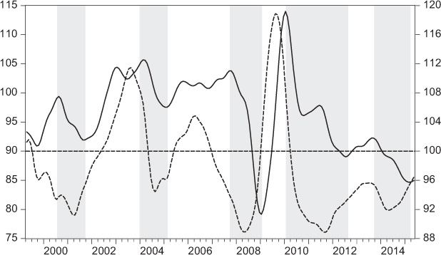
Coincident composite index (full line; Left-Vertical)
Leading composite index (dashed line; Right-Vertical)
The dashed line in Figure 1 is the leading composite index compounded by the 7 leading indicators in Table 1. The average advanced period of the peak and bottom of the leading composite index compared to the coincident composite index is 9 months and 6 months, respectively. It can be seen in Figure 1 that Apr., 2014 is valley of the latest round fluctuation of leading composite index. According to the average period of the valley of leading composite index and the characteristic of gradually increasing of the advanced period of the valley in every cycle, Jan. or Feb. of 2015 may be the valley of the current round of fluctuation of the coincident composite index. Furthermore, we can judge Chinese economic trends by Diffusion Index (DI).
2.3 Analysis of Economic Prosperity Based on Leading Diffusion Index
The coincident, leading, and lagging diffusion index are specified using prosperity indicators in Table 1. And the Chinese coincident and leading diffusion indexes are shown in Figure 2. The Diffusion Index (DI) treats the change of proportion of rising (or falling) index in indicator set as the infiltration process of prosperity. When the value of diffusion index is 50%, the rise and decline tendency of economic activity is balanced. That is to say, it is the turning point of the economic prosperity. When the diffusion index passes through the 50% line from the top to down, the previous month is the peak of the business cycle. Otherwise, when the diffusion index gets through the 50% line from bottom to top, the previous month can be regarded as the valley. Obviously, the maximum and minimum points of diffusion index appear before the peaks and valleys of business cycle, which provides us an effective way to predict the peak and valley of economic prosperity.
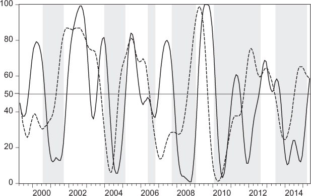
Coincident diffusion index (full line) and Leading diffusion index (dashed line)
According to Figure 2, the coincident diffusion index comes to its minimum point in Feb., 2014. But after Aug., 2014, the coincident diffusion index falls back slightly. In Apr., 2015 the coincident diffusion index gets through the 50% line from bottom to top. So Mar., 2015 is the valley of the coincident diffusion index.
After synthesizing all the results of the composite index and the diffusion index, we can make a conclusion that decline stage of the latest round of economic cycle finishes in Mar., 2015, and the cycle has stabilized and begins to take a favorable turn.
3 Prosperity Analysis by Monitoring and Warning Signal System
The Monitoring and Warning Signal System can indicate the economy condition and the trend of future economic by observing and analyzing the changes of the warning signals. So it can provide a basis for economic decision-making departments to regulate the dynamic economic operation. In this section, we select 12 economic indicators from main economic areas including industrial production, import, export, investment, fiscal revenue, financial, prices and real estate to construct Business Monitoring and Warning Signal System of China’s macro economics[4].
Signals of monitoring and warning indicators
 |
3.1 The Design of the Warning Signal System
1) The selection of warning indicators
The most primary job of establishing the Warning Signal System is to choose warning indicators. The warning indicators should reflect the scale, level and speed of the macro economy in different aspects. Specifically, the selected indicators should meet the following requirements.
First, the selected indicators must be of economic importance and represent the main aspects of economic activities. The selected indicators should be stable over a period of time. That is, warning limits of the selected indicators maintain relative stability.
Second, the selected indicators must present leading or consistency feature compared to the benchmark indicator. In other words, they are consistent with or slightly ahead of economic fluctuation so that they can sensitively reflect the economic climate.
Last, the selected indicators should be published rapidly and accurately.
The early warning indicators are in form of year-on-year growth rate. After the seasonally adjustment by X-11, we use TC series, which do not include the seasonal and irregular elements, to constitute warning signal system.
2) The determination of warning limits
The warning limits of warning signal system have four values called check points. The four check points can determinate five signals of “red”, “yellow”, “green”, “light blue” and “blue”, corresponding to the state of hot, heating, normal, cooling and cold, respectively[3]. When the value of index exceeds a certain check point, the warning signal system sends out the corresponding signal. At the same time, the system gives each signal corresponding score. Suppose that the number of warming indicators is m. Then we can sum the m indicators’ signal scores to get the composite index in every month.
According to the proportion, we translate the signal scores and composite index into centesimal measure. That is, the composite index value is in the range of 0 to 100. After then, the scores of lights are as follows:
where i is the serial number of five kinds of signal. 5, 4, 3, 2 and 1 are corresponding to hot, heating, normal, cooling and cold, respectively.
Then we judge the warning signal of every month by the check point of composite index.
3) The output of signal figure
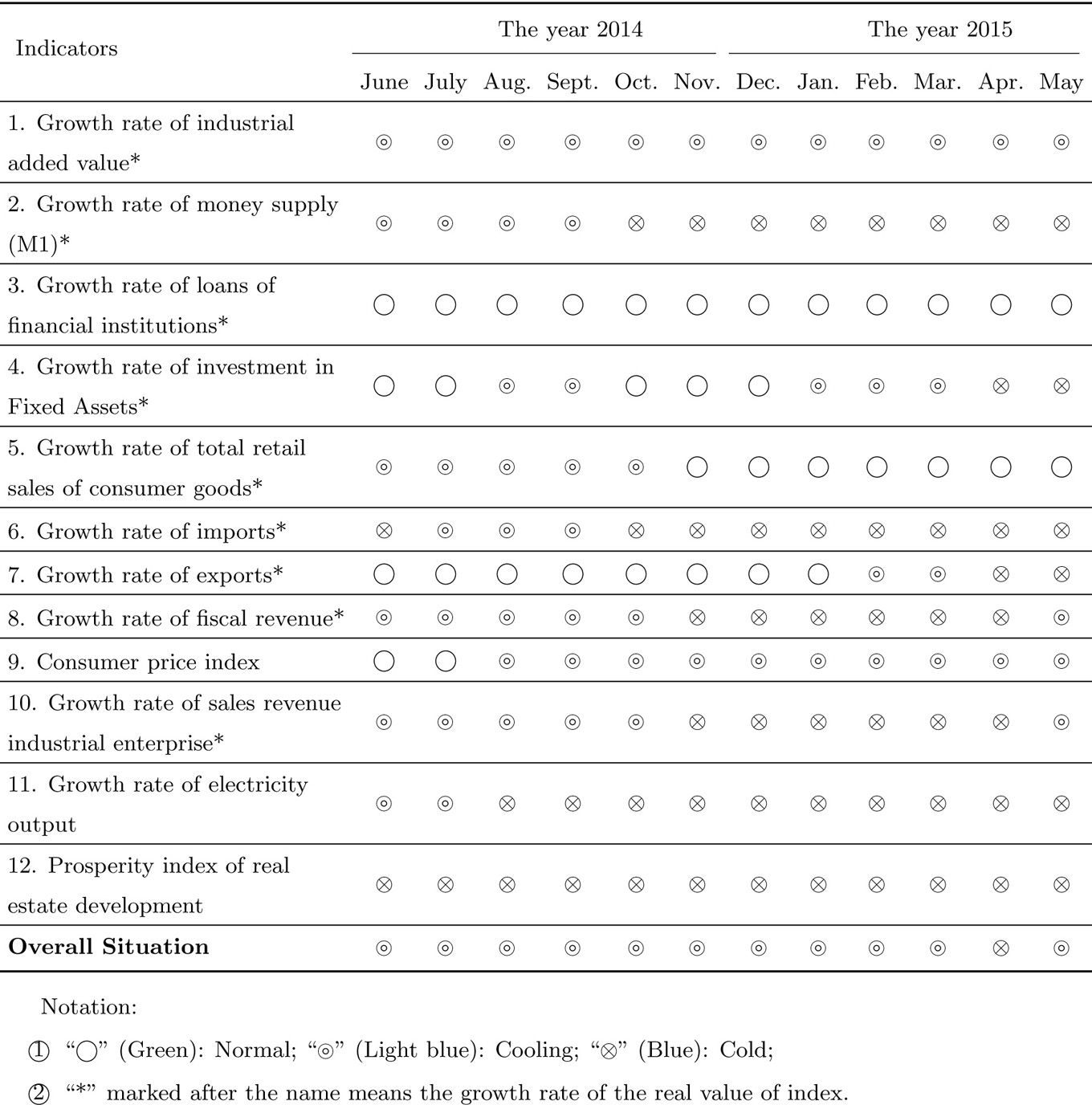
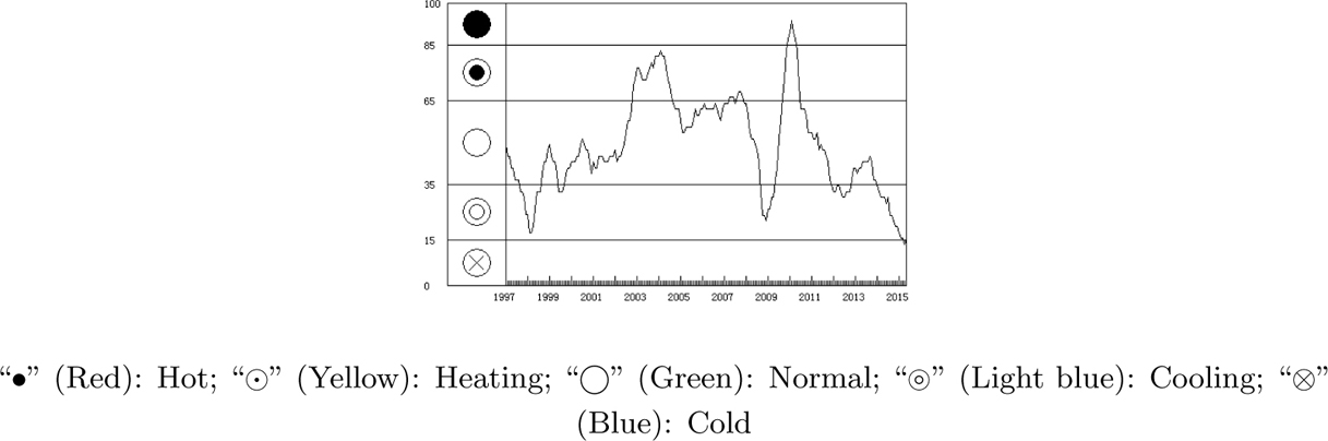
The prosperity signal figure is the result of the warning system. Figure 3 shows the variations of China’s prosperity composite index, which makes up by 12 warning indicators. Limited by the format, this paper can’t display other color. So we use different marks on behalf of the state or light type. Figure 3 shows the curve of the prosperity composite index and the area of every signal. The system can also show indicator signals (Table 2) which displays the prosperity signals of every warning indicator and prosperity composite index in every month. On one hand, we can analyze the comprehensive changes in prosperity. On the other hand, we may study the prosperity signal of every warning indicator in every month and check whether there are exceptions.
The prosperity composite index
3.2 The Analysis Based on the Prosperity Composite Index
Figure 3 shows trend of the prosperity composite index calculated by Business Monitoring and Warning Signal System. In Figure 3, the trend of the prosperity composite index is similar with the coincident composite index in Figure 1. Influenced by the world economic crisis, China’s economic growth entered the cooling “light blue” state in 1998 and 2008 respectively. The prosperity composite index is in the normal “green” state during most of the years after 1997. But the prosperity composite index experiences ups and downs between 2008 and 2012. Affected by Chinese government’s 4 trillion investments dealing with the global financial crisis, the prosperity composite index rises rapidly from cooling “light blue” to the hot “red” state from the beginning of 2009 to the beginning of 2010. And after that, the prosperity composite index slow down quickly.
Figure 3 shows that the prosperity composite index ends its decline and rises again after Aug., 2012 and reach a small peak in Aug., 2013. And then, the prosperity composite index shows downward trend in June, 2013 and enters into the cooling “light blue” area in Feb., 2014. After that the prosperity composite index stays in the cooling “light blue” area up to May, 2015.
3.3 The Analysis Based on the Signals of Monitoring and Warning Indicators
The monitoring results (Table 2) of early warning indicators show that most indicators decline from Jun., 2014 to May, 2015. The loans of financial institutions and the total retail sales of consumer goods are in the normal “green” area. The rest indicators, such as the industrial added value, sales revenue of industrial enterprise, money, are in the state of cooling or cold in May, 2015. The outcomes show that China’s economic, which is reflected by growth rate of China’s GDP, is the result of investment. And the endogenous power of economic growth is still insufficient. In general, Chinese economy has not entered the normal range of growth in the year 2015. According to the current tendency, if there is no continuous policy support, economic prosperity may be still weak in the second half of the year 2015.
1) Industrial production falling to cooling area
As the gradually implementing of motivating measures for steady growth, structural adjustment, and promoting transformation by China’s central government, the actual growth rate of industrial added value enters the normal “green” area after May, 2013. But the growth rate decline again in the year 2014. Table 2 shows that the real growth rate of industrial added value is in the state of “light blue” until May, 2015. But the sales revenue of industrial enterprise enters into the state of “blue” in Nov. 2014 and changes to “light blue” state in May, 2015.
The cooling of the current industrial production and enterprise benefit is partly due to the gloomy world economy and the weak external demand, but also to the insufficiency of effective domestic demand and excess capacity of certain industries. In addition, the promoting of industrial structure adjustment affects a certain part of the heavy chemical industry in the year 2013. In the process of eliminating backward production capacity and adjusting the industrial structure to realize high quality growth in China, the phenomenon is reasonable that the growth of industrial production slows down[4, 5].
2) Exports back to normal range in the second quarter of 2014
Improvement of export growth rate in the second quarter of 2014 drives the growth of Chinese GDP. But the export growth rate fluctuates greatly. In the first quarter of 2014, the growth rate of export is negative. To deal with the severe situation of international trade, China’s government issued a series of measures to stabilize growth of export, such as strengthening financial support to export enterprises, increasing the tax preference of import and export, stabilizing the RMB exchange rate and so on. Meanwhile, the whole environment of international trade is gradually improved. The US economy is showing signs of recovery, and Euro zone debt crisis has weakened as a whole. Owing to the motivation of Chinese domestic macro policy and the growing global demand, the real growth rate of total export sends out normal signal in Jun., 2014. Accumulated real growth rate of total import drops to cold range in the first half of 2014, but it returns to the normal area in Jun., 2014.
3) Growth of investment in fixed assets staying in a normal range
From the second half of the year 2013 to Jun., 2014, the growth rate of fixed asset investment keeps smooth and comparatively rapid, guaranteeing steady-growth of China’s economy. Facing the obvious stress of recession and the new round of “China economic collapse theory”, Chinese government did not adopt a huge economic stimulus package to maintain the rapid growth rate. In contrast, it emphasizes on the market role in competitive system to close down outdated production facilities and to reach the upgrading of company and product. Besides, China’s government adjusts the investment structure initiatively and puts the limited investment to the key areas of economic and social development. All those measures give impetus to lasting economic growth; that is, they strengthen the basis for further economic or social development. Table 2 shows that real growth rate of investment of fixed assets runs in the normal range steadily in the first half of the year 2014.
4) The growth rate of money supply (M1) staying in cooling range
In Table 2, as we can see, the growth rate of money supply (M1) removing seasonal and irregular factors stays in cooling range in the first half of the year 2014. Tight money supply growth rate has an effective correction to soaring money supply in the previous years, and would help to control inflation as well as the upward housing prices. Besides, Chinese central bank takes reasonable approach to support the developments of agriculture and small (or micro) enterprises by lowering deposit reserve ratio directionally[6]. On one hand, this measure can ensure the demand for liquidity in key areas which is also conducive to economic recovery. On the other hand, it can control the money supply growth at a lower level effectively.
5) The composite prosperity index of real estate development staying in the cold area
Obviously, the composite prosperity index of real estate development is the cyclical indicator reflecting real estate development. Owing to the continuous controls on the real-estate sector, the composite prosperity index of real estate development is in cold “blue” area in the first half of the year 2014.
Tight mortgage, high house prices, heavy taxes and fees lead to the low sale growth of commercial houses, the accumulation of housing inventories, and the frustration of real estate developers’ enthusiasm. Combined with factors as the financing difficult in real estate business, all those factors make the composite prosperity index of real estate development stay in the cold range. As is well known, real estate investment contributes a lot to Chinese economic growth because the growth of the real estate development can boost many relative industries[7]. Therefore, the low growth rate of real estate investment may further exert the downward pressure on economic growth.
4 Conclusions
In this paper, the monthly real growth rate of industrial added value indicator released by the China National Bureau of Statistics was chosen to be the benchmark index. We collected a large number of macroeconomic indicators and got the actual value of economic indicators through deflating by multiple price indexes. On this basis, 26 indicators from various areas of the economy were regarded as China’s macro economic prosperity indicators by using methods such as K-L approach, time difference correlation analysis and grading system. These 26 indicators corresponded well with the fluctuations of benchmark index. Furthermore, we analyzed and forecasted the economic growth rate cycle of China in the second half of the year 2014 by composite index method and early warning signal system to understand the change in the macroeconomic situation. Through the analysis of warning signal of the warning indicators, we can analyze the causes of economic fluctuations. Moreover, through the analysis of leading composite and diffusion index, we found that China’s macroeconomic growth cycle began to enter into a new round of short cycle period of slow decline from Sept., 2013 (peak) and arrived the bottom in Aug., 2014.
The above analysis suggested that the fluctuation of China’s growth rate cycle is considerably large in recent 17 years. But after 2012, the macroeconomic growth has the characteristics of low and small wave motion. As China’s economy still faces downward pressure, the central bank should reduce interest rates and Reserve Requirement Ratio timely to ease enterprise’ difficulty in financing and reduce the social cost of financing effectively. The government should adopt positive measures to guarantee the economic operation and maintain a good situation of medium growth and low inflation.
References
[1] Chen L, Sui Z L. Analysis and forecasting on the business cycle and price fluctuation from 2013 to 2014. Economy of China Analysis and Forecast (2014), Beijing: Social Science Academic Press, 2013.10.31193/ssap.isbn.9787509740293Search in Google Scholar
[2] Dong W Q, Gao T M, Chen L, et al. Analysis and forecasting methods of economic cycles. Changchun: Jilin University Press, 1998.Search in Google Scholar
[3] Kong X L, Gao T M, Zhang T B. Analysis and forecasting on the macro economic business cycle fluctuation in 2014. Analysis on the Prospect of China’s Economy (2014), Beijing: Social Science Academic Press, 2014.Search in Google Scholar
[4] Jia K. The characteristics and four bright spots of macro-control in the first half of the year. People’s Net, http://theory.people.com.cn/n/2014/0721/c40531-25305451.html.Search in Google Scholar
[5] Zhang L Q. Analysis and forecasting on the economic situation from 2013 to 2014 — The growth rate of China has enter into the interval of 7%∼8%. Economic Perspectives, 2014(1): 4–8.Search in Google Scholar
[6] Li reiterated the new guidelines of macro-control should take a drip irrigation and no flood style. Xinhua Net, http://www.hn.xinhuanet.com/2014-07/21/c-1111709810.htm.Search in Google Scholar
[7] Experts illustrate the economy’s bright spots in the first half of the year 2014-micro stimulation and restructuring become effective. China News Net, http://finance.chinanews.com/cj/2014/07-21/6406776.shtml.Search in Google Scholar
Indicators of Business Monitoring Warning Signal System and their warning limits
| Indicators | Red light | Yellow light | Green light | Light blue light | Blue light | |
|---|---|---|---|---|---|---|
| Hot | Heating | Normal | Cooling | Cold | ||
| 1. Growth rate of industrial added value * | ← | 15.0 | 13.0 | 9.0 | 6.0 | → |
| 2. Growth rate of money supply (M1) * | ← | 20.0 | 16.0 | 8.0 | 3.0 | → |
| 3. Growth rate of loans of financial institutions * | ← | 20.0 | 17.0 | 11.0 | 7.0 | → |
| 4. Growth rate of investment in Fixed Assets * | ← | 26.0 | 22.0 | 14.0 | 10.0 | → |
| 5. Growth rate of total retail sales of consumer goods* | ← | 18.0 | 16.0 | 11.0 | 9.0 | → |
| 6. Growth rate of imports * | ← | 23.0 | 20.0 | 5.0 | 3.0 | → |
| 7. Growth rate of exports * | ← | 24.0 | 20.0 | 5.0 | 2.0 | → |
| 8. Growth rate of fiscal revenue * | ← | 26.0 | 20.0 | 8.0 | 4.0 | → |
| 9. Consumer price index | ← | 6.0 | 5.0 | 2.0 | 0.0 | → |
| 10. Growth rate of sales revenue industrial enterprise* | ← | 25.0 | 20.0 | 10.0 | 7.0 | → |
| 11. Growth rate of electricity output | ← | 16.0 | 14.0 | 5.0 | 3.0 | → |
| 12. Prosperity index of real estate developmentm | ← | 105 | 103 | 100 | 97 | → |
| Composite index | ← | 85 | 65 | 35 | 15 | → |
Notation: The numbers in appendix 1 are growth rates and their measurement units are “%” excepting two indicators No. 9 and No. 12.
© 2016 Walter de Gruyter GmbH, Berlin/Boston
Articles in the same Issue
- Review on Financial Innovations in Big Data Era
- The Indicator Selection and Monitoring Analysis of Growth Rate Cycle in China
- Research on Investment Preference and the MAX Effect in Chinese Stock Market
- An Optimal Emission Mechanism of Sustainability of China: How to Achieve a Win-Win Solution Between Economy and Environment?
- Analysis of a Single-Sever Queue with Disasters and Repairs Under Bernoulli Vacation Schedule
- New Results on Multiple Solutions for Intuitionistic Fuzzy Differential Equations
- Multiattribute Decision Making Method Based on Intuitionistic Linguistic Aggregation Operator