A New Investor Sentiment Indicator Based on Return Decomposition

1 Introduction

The concepts of noise trader and investor sentiment were introduced into the research scope of standard finance when Black, a famous economist, published the paper “Noise”^[1]. Black emphasized the enormous weighting of noise trader in financial market, and asserted that it was noise trader that constantly provided market with liquidity supply. In 1990, De Long, Shleifer, Summers and Waldmann introduced the noise trader with sentiment characteristics into the traditional pricing model for the first time, creatively establishing DSSW model^[2] and clarifying the possibility of long-term presence of arbitrageurs and noise traders and their role in pricing. In the last decade, people gradually discover that the classical finance theory is challenged by financial market anomalies from time to time^[3-6], whereas the emerging behavioral finance theory can provide an incomparably sound explanation in comparison with the classical ones^[7-9]. And increasing research results indicate that investor sentiment has a noticeable effect on the formation of asset price and liquidity supply^[10-13].

However, the trouble many researchers are facing with is that no optimal indicator or proxy variable is available to measure investor sentiment. Part of the traditional proxy variables often result in conflicting empirical results. In addition, it is hard for us to timely understand the level of investor sentiment in market today, since some classical proxy variables for investor sentiment have a long release cycle (e.g., monthly or quarterly). More importantly, almost all the classical proxy variables for investor sentiment^[14-16] can only measure the average level of investor sentiment in market and as a result the pessimistic and the optimistic cannot be distinguished (obviously these two sentiments always exist in market simultaneously). To this end, a new proxy variable for investor sentiment is proposed based on high frequency trading intraday data. This variable represents investor sentiment of individual share or financial market on daily frequency, and the pessimistic and the optimistic are distinguished. Then the relevance between the proposed variable and the traditional proxy variables for investor sentiment is examined, in which way the rationality of the proposed variable is clarified. Finally, based on the new proxy variable for investor sentiment, we find that investor sentiment is one of the important causes of “idiosyncratic volatility” and “mispricing” phenomenon.

2 Methodology

Firstly, the DSSW model is extended such that it can accommodate three different types of investors simultaneously: Rational arbitrageurs, optimistic investors and pessimistic investors. Specifically, suppose the mispricing levels of optimistic investor and pessimistic investor on the tth trading day are, ρto>0,ρtp>0, respectively. Following the assumption of DSSW, the exponential utility functions of three different types of investors are the same, i.e., U(w) = e^-2γw, at the same time, simple-period decision is assumed, i.e., maximizing the expect of utility function: E_t(U(w_{t + 1})). When the asset’s future price satisfies normal distribution, exponential utility function will be proportional to the expected total revenue and inversely proportional to the conditional volatility. Therefor the equivalent decision equation is

where Equation (1) are the decision equations for rational arbitrageurs, optimistic investors and pessimistic investors respectively, C_t is the initial value, rt0 is risk-free rate of return, σt+12 denotes the conditional variance of asset price on the (t + 1)th trading day. The first-order conditions of the solutions can be given as follow respectively,

Similar to DSSW model, the proportion of the three types of investors are assumed to be, 1 - μ^o - μ^p, μ^o, μ^p, and riskless assetelasticity is infinite, supply of risk assets being 1. One can obtain the equilibrium price from the aforementioned equation as follows

Since the data are obtained daily, risk-free rate will be very small and consequently rt0=0 is assumed. Equation (3) can be put into an equivalent form, given by

where I_t is the information-driven price fluctuations of rational arbitrageurs, ItoandItp are sentiment-driven price fluctuations of optimistic investors and pessimistic investors respectively.

Generally speaking, daily return based on close price is the summation of the three terms. As a result, it is impossible to distinguish the price fluctuations driven by three different types of investors on daily frequency. However, daily high frequency data can provide us with a possible solution based on the idea of return decomposition. In this approach, we assume that rational arbitrageurs actively collect all relevant information about asset prices and quickly implement their trading strategies based on a specific risk appetite. Investor sentiment, as an inherent property of traders, will continue to lead to price volatility until closing. Following the idea of Tetlock^[11], we assume that the overnight information of asset prices will be released after the opening within a very short time (e.g., 60 minutes), impacting the market in the form of I_t, whereas a large number of day volatility due to the sentiment of the latter two types of traders are slowly released, eventually leading to return rate (at closing time).

To this end, we assume the logarithmic asset prices on the tth trading day satisfies Ito process

where the drift term, astds, satisfies limited variation process, σst is the stochastic variation rate, and wst is a brown motion. astds can be divided into two monotonic function of the incremental difference

where GstandBst are monotonic function, and Gst+Bst=Vξ=0sAξ,Aξ=∫0ζaτtdτ. The existence and uniqueness of the aforementioned decomposition can be proven. We find that the smooth portions of logarithmic intraday price volatility can also be regarded as slow release, i.e.,

It can be discovered that the evolution characteristics and economic significance of Gst(Bst) is similar to the release process of investors’ sentiment (the optimistic or the pessimistic). Consequently, we believe that GCloset=Gt(BCloset=Bt) can be seen as an approximation of Ito(−Itp).

We then design a set of specific solving scheme for G_t(B_t) based on the five-minute-high-frequency trading data (return, buyer dominate volume and seller dominate volume). Since the trading mode is implemented by order book in China at the stage of continuous auction, the daily price fluctuations can be decomposed into two parts, i.e., price impact driven by order book, random drift of order book. However, the weighting of the former is larger than that of the latter substantially (bid-ask bounce, one of the most important daily price fluctuations, can be seen as a special case of the former one). Specifically, the limit-order on the order book following the principle of price preference and time preference is activated when a market-order is reached, thus promoting the rise (or drop) in asset prices.

Similar to the non-liquidity ratios proposed by Amihud^[17], the price impact generated by the above procedure is approximately expressed as a linear function of turnover, given by

where ILtaskandILtbid denote non-liquidity ratios of seller’s order book and buyer’s respectively, dvt,sbanddvt,ss denote instantaneous state of buyer dominate volume and seller dominate volume. To simplify the model, we further assume that, ILtaskandILtbid are constant in one day. It should be noted that ILtaskdvt,sb,ILtbiddvt,ss is incremental difference of two monotonic functions.

Compared with (7), and in conjunction with the physical meaning of ILtask,ILtbid,dvt,sbanddvt,ss, one can obtain

They will be a descent approximations of G_t and B_t, i.e.,

where vt,kbandvt,ks are the kth five-minute buyer dominate volume and seller dominate volume on the tth day respectively. Finally, in order to calculate the non-liquidity ratios ILtask(ILtbid), and consequently to get the value of G_t(B_t), least squares estimation is performed on the following equation

where b^1andb^2 are used as the approximations of ILtaskandILtbid. In this way, we can obtain the sentiment proxy variable for any securities (or its combination) under daily frequency and the pessimistic and the optimistic can also be distinguished.

3 Data Sources and Descriptive Statistics

The table data come from Tinysoft Data Service Platform. This table shows the descriptive statistics of different data. The data herein are composed of daily data set and high frequency data set during 4th January, 2013 to 31th December, 2013, where the former is a total of 238 data sets for the SSE Composite Index trading logarithmic return rate, the latter covers logarithmic return rate, buyer dominate volume and seller dominate volume of all the constituent stocks among the SSE 50 Index in the frequency of five minutes. R_t denotes SSE Composite Index trading logarithmic return rate on the tth trading day. r_i,t,n denotes the logarithmic return rate of stock i in the nth five minutes on the tth trading day. vi,t,nbandvi,t,ns denote buyer dominate volume and seller dominate volume of stock i in the nth five minutes on the tth trading day.

4 Comparisons with Conventional Investor Sentiment Index

Currently, the commonly used investor sentiment indicators in China are divided into two categories, one of which is a direct sentiment indicator, including: BSI index of CCTV 2, bull and bear index of stock market trend analysis weekly, cninf investor confidence index, Yale-CCER investor confidence index of Chinese stock market and consumer confidence index^[18]. The second category is indirect indicator of investor sentiment, such as IPO volumes, IPO initianl return, new A-share accounts ratio, Shanghai Composite turnover rate, and closed-end fund discount.

The proposed investor sentiment indicator is now compared with some traditional ones, and attention is focused on the commonalities and differences between them. Specifically, three traditional investor sentiment variables are chosen, including new A-share accounts ratio, Shanghai Composite turnover rate, and closed-end fund discount.

The status of financial market is related to the number of participants, the new A-share accounts ratio is a reflection of investor sentiment naturally.

Shanghai Composite turnover rate not only reflects the market liquidity, but also the level of participation of investors. The more positive the investor sentiment is, the more frequent the fair market turnover will be, and so liquidity will be increased. Closed-end funds cannot be purchased or redeemed in a closed period, and its transaction price reflects investors’ expectations of future asset prices. If the discount rate drops, then it means that investors are optimistic about the earnings outlook of listed companies and thus assess asset prices positively, resulting in the optimistic, and vice versa.

Following the research approaches by Baker and Wurgler^[19], principal component analysis (PCA) is performed on investors’ optimistic and pessimistic indicators including their amplitude and direction, the latter one is also compared with closed-end fund discount and summarized in Figure 1.

Figure 1

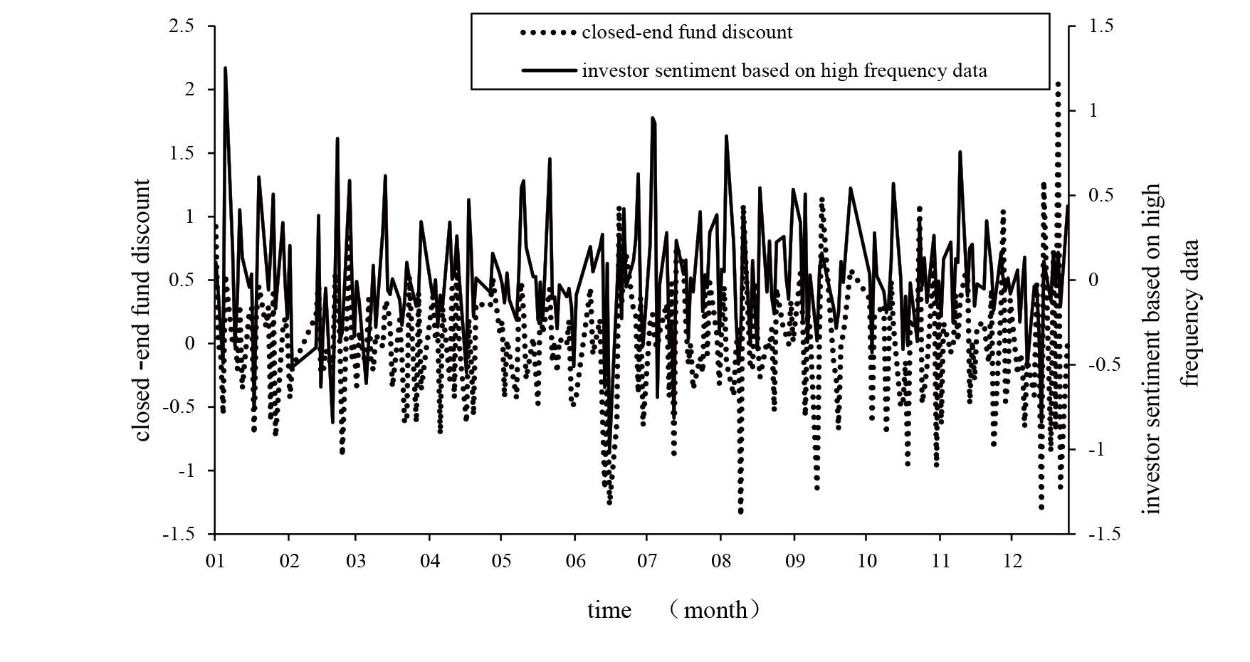
The measurement of investor sentiment

One can obtain from Figure 1 that there is a strong correlation between investor sentiment based on high frequency data and closed-end fund discount, both of which remain the same trend during the year.

The table data come from Tinysoft Data Service Platform. This table shows OLS estimates of the coefficient, which represents the impact of new A-share accounts ratio, Shanghai Composite turnover rate and closed-end fund discount to conventional investor sentiment index respectively. ***denotes significance on the 1% confidence level.

One can obtain from Table 2 that the regression coefficient between the sentiment indicators calculated from high-frequency data and A-share accounts was not significant, and wald test rejects the null hypothesis of zero coefficient. That means the number of new A-share account is only a measure of investor attention representing the amplitude of the sentiment, but cannot represent its direction.

The regression coefficient of optimistic indicator to Shanghai Composite turnover is significantly positive, while the regression coefficient of pessimistic indicator is not significant. In fact, buyer liquidity turns weak rapidly with pessimistic market sentiment. Then equal amounts of trading volume will make a bigger impact on price. However, turnover rate contains information of trading volume only, it could not measure the liquidity of order book. Therefore, we could not capture the pessimistic well.

The regression coefficient of optimistic indicator to closed-end fund discount difference is positive significantly, while the regression coefficient of pessimistic indicator is negative significantly. This means the investor sentiment indicator based on high frequency data could explain the variation of closed-end fund discount. On the other hand, closed-end fund discount is not only a proxy for the amplitude of the sentiment, but also for its direction. That’s why it is a better measure indicator for investor sentiment.

We can obtain from the comparison results that: There is a strong correlation between the sentiment indicator obtained from high frequency data and the traditional ones. However, compared to the traditional one, the proposed on based on high-frequency data can not only measure the sentiment amplitude but also its direction.

5 Empirical Research

The classical financial thesis believe that the actual price of a stock will fully reflect its intrinsic value, however in the actual financial market, noise trader is widespread and then make the stock price deviate from its intrinsic value. On the other hand, in the previous studies, it has been reported that asset mispricing is one of the best interpretations for marketing anomalies, including scale effect,inertial effect and reversal effect. Thus to investigate the effects of investor sentiment on the mispricing is significant in the researches and market guiding. We base on the classical CAPM models and strip out the non-systematic risk of assets.

where r_i,t and r_M,t are the return rate of stock i at time t and marker return respectively. r_f,t is the risk-free rate, β_i is the risk premium for factor i. And then we get the estimated risk-adjusted return in (13):

Thereafter, we would use G_t and B_t as explanatory variables and construct a time-series model and a cross-section model which could be used to explore the correlation of investor sentiment, idiosyncratic volatility and mispricing.

6 Conclusions

The contributions of the paper are summarized as follows. Firstly, the DSSW model is extended such that it can accommodate three different investors simultaneously: rational arbitrageurs, optimistic investors and pessimistic investors. Secondly, the daily return based on close price is broken down into three parts: information-driven price fluctuations of rational arbitrageurs, sentiment-driven price fluctuations of optimistic and pessimistic investors. Thirdly, a pair of good approximation of the optimistic and the pessimistic is achieved by modeling the price impact using daily high frequency data. A new investor sentiment indicator is proposed based on return decomposition, the new sentiment indicator has high correlation with other traditional ones, and as a proxy variable of individual share or financial market on daily frequency, it could distinguish the optimistic and the pessimistic. Compared with traditional ones, the new indicator can not only measure the amplitude of the sentiment but also its direction.

In terms of empirical research, a time-series model and a cross-section model are established respectively to explore the explanatory power of investor sentiment to idiosyncratic volatility and capital asset mispricing, treating the optimistic and the pessimistic as the expansionary variables. The result shows that the new sentiment indicator could explain 21.31 percent of idiosyncratic volatility to individual share on average, and it has a great explanation of 36 percent to capital asset mispricing.

References

[1] Black F. Noise. Journal of Finance, 1986, 41(3): 529-543.10.1002/9781119203070.ch14Search in Google Scholar
[2] De Long J B, Shleifer A, Summers L H, et al. Noise trader risk in financial-markets. Journal of Political Economy, 1990, 98(4): 703-738.10.1086/261703Search in Google Scholar
[3] Mehra R, Prescott E C. The equity premium — A puzzle. Journal of Monetary Economics, 1985, 15(2): 145-161.10.1016/0304-3932(85)90061-3Search in Google Scholar
[4] Campbell J Y, Shiller R J. Cointegration and tests of present value models. Journal of Political Economy, 1987, 95(5): 1062-1088.10.3386/w1885Search in Google Scholar
[5] Shiller R J. Theories of aggregate stock-price movements. Journal of Portfolio Management, 1984, 10(2): 28-37.10.3905/jpm.1984.408954Search in Google Scholar
[6] Shiller R J. Market volatility and investor behavior. American Economic Review, 1990, 80(2): 58-62.Search in Google Scholar
[7] Shefrin H, Statman M. Behavioral capital-asset pricing theory. Journal of Financial and Quantitative Analysis, 1994, 29(3): 323-349.10.2307/2331334Search in Google Scholar
[8] Shefrin H, Statman M. A behavioral framework for expectations about stock returns. Journal of Finance, 1994, 49(3): 1096-1097.Search in Google Scholar
[9] Shefrin H, Statman M. Behavioral portfolio theory. Journal of Financial and Quantitative Analysis, 2000, 35(2): 127-151.10.2307/2676187Search in Google Scholar
[10] Fang L, Peress J. Media coverage and the cross-section of stock returns. Journal of Finance, 2009, 64(5): 2023-2052.10.1111/j.1540-6261.2009.01493.xSearch in Google Scholar
[11] Tetlock P C. Giving content to investor sentiment: The role of media in the stock market. Journal of Finance, 2007, 62(3): 1139-1168.10.1111/j.1540-6261.2007.01232.xSearch in Google Scholar
[12] Ho C, Hung C H. Investor sentiment as conditioning information in asset pricing. Journal of Banking & Finance, 2009, 33(5): 892-903.10.1016/j.jbankfin.2008.10.004Search in Google Scholar
[13] Liu S M. Investor sentiment and stock market liquidity. Journal of Behavioral Finance, 2015, 16(1): 51-67.10.1080/15427560.2015.1000334Search in Google Scholar
[14] Lee C M C, Shleifer A, Thaler R H. Investor sentiment and the closed-end fund puzzle. Journal of Finance, 1991, 46(1): 75-109.10.3386/w3465Search in Google Scholar
[15] Baker M, Stein J C. Market liquidity as a sentiment indicator. Journal of Financial Markets, 2004, 7(3): 271-299.10.3386/w8816Search in Google Scholar
[16] Cornelli F, Goldreich D, Ljungqvist A. Investor sentiment and pre-IPO markets. Journal of Finance, 2006, 61(3): 1187-1216.10.1111/j.1540-6261.2006.00870.xSearch in Google Scholar
[17] Amihud Y. Illiquidity and stock returns: Cross-section and time-series effects. Journal of Financial Markets, 2002, 5(1): 31-56.10.1017/CBO9780511844393.010Search in Google Scholar
[18] Brown G W, Cliff M T. Investor sentiment and asset valuation. Journal of Business, 2005, 78(2): 405-440.10.1086/427633Search in Google Scholar
[19] Baker M, Wurgler J. Investor sentiment and the cross-section of stock returns. Journal of Finance, 2006, 61(4): 1645-1680.10.3386/w10449Search in Google Scholar
© 2016 Walter de Gruyter GmbH, Berlin/Boston
Articles in the same Issue
- The Case for Technobiology: A Complement to Biotechnology