Aspects of cavity engineering in THz quantum cascade laser frequency combs
-
Lukas Seitner

 ,
Michael A. Schreiber
,
Michael Rinderle
,
Niklas Pichel
,
Michael Haider
and
Christian Jirauschek
,
Michael A. Schreiber
,
Michael Rinderle
,
Niklas Pichel
,
Michael Haider
and
Christian Jirauschek

Abstract
Terahertz quantum cascade laser (QCL) frequency combs are a disruptive technology for spectroscopy, imaging, and quantum technologies in this spectral range. For advanced development and tailoring of frequency comb properties, detailed modeling of the QCL device is necessary. Recent achievements in the field of THz QCLs have unveiled that custom modifications of the laser cavity by dispersion engineering or tapered waveguide sections significantly influence the laser’s behavior. In this article, we present a numerical model based on the Maxwell-density matrix formalism that captures such cavity effects in detail, yielding a better understanding of the QCL dynamics and opening the possibility of designing cavities for custom laser applications. We show that waveguide engineering in terms of dispersion compensation and field enhancement can stabilize an unlocked multimode state into frequency comb operation and even shape its properties, such as the bandwidth or the mode spacing of harmonic frequency combs.
1 Introduction
The terahertz portion of the electromagnetic spectrum has increasingly attracted many research activities, aiming to develop improved emitters and detectors that can potentially unlock a wide range of applications [1]. Using this spectral band for sensing, imaging, security, or communication requires high-power, portable, and ideally coherent sources. Somewhat more than 30 years ago, the quantum cascade laser (QCL) was demonstrated in the mid-infrared, potentially fulfilling these requirements [2]. The name refers to its active region design, which is based on a semiconductor heterostructure with alternating conduction band offset and engineered intersubband levels. Some years later, this technology was transferred to the THz range, with the first laser operating at
The numerical modeling of QCL frequency combs is typically based on Maxwell–Bloch equations, which couple the propagation of the electric field in one spatial dimension to the active region dynamics [18], [19], [20]. Many efforts were made to successfully describe the intersubband charge carrier transport and gain properties by rate equations, the Monte-Carlo method, or the nonequilibrium Green’s function formalism [21], [22]. Recent dynamical models cover a broad range of complexity, spanning from multilevel density matrix and full-wave field solvers to effective master equations and semi-analytic mean field theories [23], [24], [25], [26], [27], [28]. These spatiotemporal models are especially suited for including cavity modifications, such as defects, microwave copropagation, or saturable absorbers [29], [30], [31], [32], [33].
Previous theoretical work based on Maxwell–Bloch-type equations has primarily focused on the modeling of the QCL active region, while advanced waveguide structures beyond standard Fabry–Perot or ring cavities have rarely been considered. Notable exceptions include the implementation of air slits [29], an external cavity [27], or a distributed feedback grating [34]. In the present work, we discuss a general numerical model for QCLs with multiple sections, potentially featuring different refractive indices, changing waveguide widths, and complex-valued reflection and transmission coefficients. Thus, experimentally realized structures, such as Gires–Tournois interferometers [35], [36] or tapered cavities [37], can be treated consistently within the numerical Maxwell-density matrix framework [24]. With that, we unravel the influence of cavity engineering on frequency comb formation and the shaping of the temporal and spectral characteristics of the electric field. Our results bring relevant insights into dispersion engineering and field enhancement by waveguide modification and their influence on the active region dynamics. The developed model is consistent with recent experimental results and can be used for laser analysis and design in future work.
2 Theoretical model and numerical implementation
Usually, Maxwell–Bloch-type models for QCL simulation consist of three parts. Thereby, the propagation of the electric field is coupled to the microscopic charge carrier dynamics via the medium polarization. Finally, boundary conditions, which represent the properties of the cavity, complete the model. This section introduces the electric field model and its numerical implementation in a possibly defect-engineered or tapered cavity.
2.1 Electric field and medium polarization
In an actual QCL device, the electric field is a three-dimensional quantity. However, the active region only amplifies the out-of-plane component of the electric field, such that transverse magnetic modes are enforced. By using the slab waveguide approximation, i.e., assuming the transversal field distribution to be invariant along the waveguide, a one-dimensional description of the time-dependent electric field E(x, t) in its propagation direction x is sufficient to capture the laser dynamics, significantly reducing the numerical load [24]. Moreover, we assume that the field envelope varies slowly compared to the carrier frequency. In this slowly varying envelope approximation (SVEA), the field is decomposed into two counterpropagating components E ±(x, t), according to the ansatz
where ω
c = 2πf
c denotes the center frequency. Furthermore,
derived from Maxwell’s equations. Here, v
g denotes the group velocity and β
2 is the background group velocity dispersion (GVD). Furthermore, the optical power loss is given by a, and the term
Here,
2.2 Reflection and transmission
Partial reflection and transmission processes of the electric field play a pivotal role in THz QCLs because the dimensions of (sub-)cavities might be in the range of the intracavity wavelength of ≈ 15–70 µm, and thus influence the operation. This opens up the possibility to engineer the waveguide for beneficial properties, such as dispersion compensation or frequency filtering. The Maxwell–Bloch-type equation system described above is complemented with explicit boundary conditions for the optical field that are, in our case, defined by the laser cavity. In a linear waveguide, we have a finite field reflection at the two facets, while a ring cavity is described by periodic boundary conditions.
2.2.1 Changing refractive index
Focusing on field reflections at a material interface and considering normal incidence, the Fresnel formulas yield the reflection and transmission coefficients
with n 1 and n 2 being the effective refractive indices of the two materials. For the facet of a QCL laser cavity, typical values for the semiconductor material are n 1 ≈ 3.3 and n 1 ≈ 3.6 for mid-IR and THz QCLs, respectively. In case of air surrounding the waveguide (n 2 = 1), this results in a power reflection of R 12 = |r 12|2 ≈ 0.3, such that the power outcoupling T 12 = 1 − R 12 ≈ 0.7. However, for metal–metal waveguides in the THz range, the reflection is typically significantly larger than expected from Fresnel’s formula (R 12 ≈ 0.6 − 0.8). In that case, wave-optical effects depending on the exact geometry considerably influence the electromagnetic behavior [41]. Depending on the model requirements, r 12 can be extracted from three-dimensional electromagnetic simulations or analytical models [21]. At this abrupt change from a guided mode profile to free-space propagation the power still must be conserved, such that the relation
holds, if no losses occur.
However, reflections and a changing refractive index can also happen inside the laser cavity and thus within the simulation domain. For the implementation of a reflection in the SVEA model, a phase correction term must be added to the reflection process. As the electric field is modeled by two counterpropagating complex amplitudes with counter-rotating spatial phasors [Eq. (1)], E
+ and E
− possess a spatially dependent phase difference equal to
Here, r ± represents the reflection coefficient for the respective field direction.
Simulating several regions with varying effective refractive indices might be necessary, e.g., to model an external cavity reflector or the air gap in an integrated laser/detector setup [42]. The numerical solution of Eq. (2) using the RNFD scheme of Eq. (3) including a material interface at location x
r is illustrated in Figure 1. In this scenario, E
+ is propagating from n
1 toward n
2, such that the coefficient r
+ refers to r
12 and consequently r
− refers to r
21. The used abbreviations
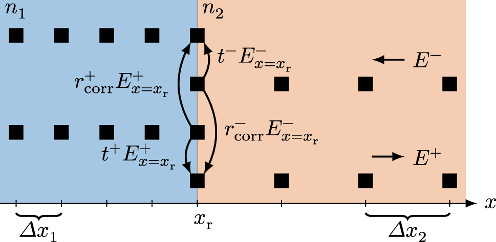
Spatial discretization of the simulation domain close to an interface of two materials with different refractive index. The two upper rows represent the grid points of the left-traveling field, while the two lower rows account for the right-traveling field. A double grid point at the interface ensures a consistent treatment of reflection and transmission processes.
The interface implementation is tested by a double interface in a ring cavity, where we can easily compare reflected and transmitted portions of the initial pulse after several round trips. The envelope approximation introduces the same type of phase error when modeling ring cavities. At the beginning and end of the simulation domain, i.e., where the ring gets closed, the full-wave electric field needs to be continuous, such that the complex envelopes at that point need to be phase-corrected by
where L is the circumference of the ring. As a numerical example, we use a 200 µm section of the polymer benzocyclobutene (BCB) with refractive index n 2 ≈ 1.57, used for planarized THz QCL platforms [43], in between two GaAs regions with n 1 = 3.6. In Figure 2, the pulse is visualized while partially reflected and transmitted at the material interfaces. In (a), the amplitudes and phases of the right and left traveling components are shown, as calculated in the SVEA, and behave rather unintuitively due to the phase correction terms. However, from Figure 2b, it becomes clear that the correction terms are essential to be considered at interfaces in the SVEA. There, the full-wave electric field reconstructed by Eq. (1) is plotted, showing the expected behavior with phase continuity, longer wavelength, and increased amplitude due to the reduced refractive index.
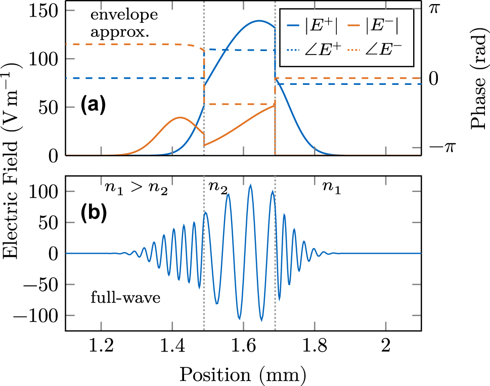
Spatially resolved electric field at a double material interface. (a) Amplitude and phase of both field components in the envelope approximation showing nontrivial behavior. (b) The reconstructed full-wave electric field at the interface is continuous but changes amplitude and frequency according to the refractive index change.
To validate the numerical implementation, we analytically calculate the frequency-dependent reflection and transmission coefficients for electromagnetic propagation through a thin gap by [44]
where
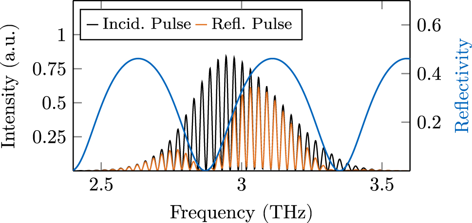
Reflected and transmitted pulse spectrum after interacting with a double facet, compared to the analytically calculated reflectivity. The correct frequency dependence is obtained by applying the phase correction terms outlined in the main text.
2.2.2 Changing waveguide geometry
One advantage of the SVEA model is the possibility to include effective reflection and transmission coefficients beyond the Fresnel relations, which is not straightforwardly possible in full-wave simulations. Therefore, one can include reflections in the one-dimensional model, which are not related to a refractive index change along the propagation direction. For example, the waveguide width might abruptly increase to realize contacting pads in a ring cavity [45]. In that case, the effective refractive index will only vary minimally, while strong field reflections occur at the sudden impedance change. Moreover, those pads present facets to the air, where significant outcoupling occurs that might be relevant for the model. For such a scenario, r needs to be determined individually, and the transmission coefficient can be calculated by t
± = 1 + r
± − l, where
2.3 Tapered waveguide sections
Apart from abrupt changes in the refractive index or the cavity geometry, the waveguide can be designed to change its width gradually, leading to field enhancement by the tapering effect. Thereby, the transverse mode profile can be assumed to adapt adiabatically, such that it is directly compatible with the one-dimensional model. We include the taper by an effective position-dependent intensity loss coefficient a t(x), which can also act as an amplification for a t < 0. In the propagation equation (2), it is considered by adding a t to the overall optical power loss a. For an adiabatic linear taper, we obtain (see Appendix)
where α = w 2/w 1 is the tapering factor, i.e., the ratio between the waveguide width at the end (w 2) and the beginning of the tapered section (w 1). Furthermore, x 1 and x 2 refer to the position in the field propagation direction where the tapering starts and ends, respectively. The layout of a tapered cavity device is visualized from the top view in Figure 4a, along with the relevant parameters.
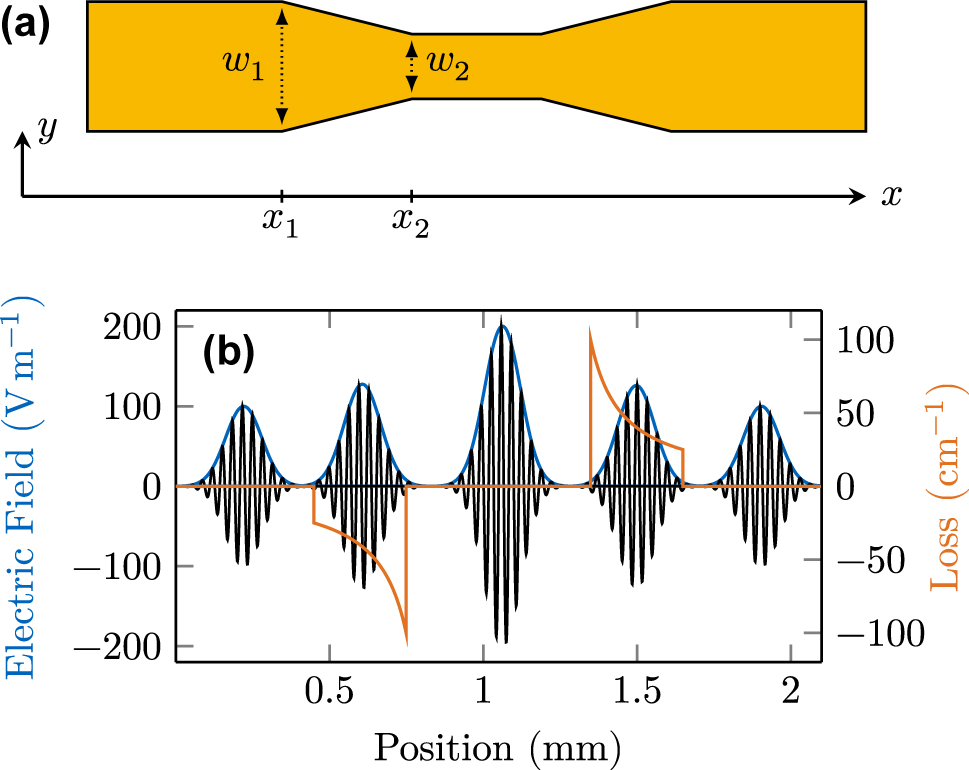
Tapered waveguide sections for field enhancement. (a) Top view of a tapered laser cavity. (b) Gaussian pulse propagating through the tapered cavity, seeing consecutive intensity gain and loss.
To test the implementation, we seed a 1 ps pulse in a cavity without gain medium and observe its propagation behavior. We choose a tapering section with α = 0.25 for field enhancement and another one with α = 4 for consecutive amplitude reduction, both with a length of 300 µm. As
In conclusion, the linear tapering of a waveguide can be included in numerical simulations rather easily but can have a significant influence on QCL operation and its coherence, as we will discuss in Section 3.3.
3 QCL dynamical simulations
In this section, we apply the previously discussed cavity engineering techniques to QCL simulations and observe their influence. We show that careful design can lead to phase locking of an otherwise unlocked multimode state. As a first step, we develop an active region description suitable for our model.
3.1 Active region design
A QCL active region consisting of a multi-quantum-well heterostructure achieves optical gain by field interaction with intersubband transitions in the conduction band. Population inversion between the upper and lower laser levels (ULL/LLL) is ensured by carefully designing the heterostructure’s layer sequence and applying a suitable bias. We include the effect of this gain medium into our model by coupling the corresponding density matrix equations in the rotating-wave-approximation (RWA) to the propagation equation (2), via the polarization term f ± [24], [49]. Required parameters include energy levels, coupling energies of tunneling transitions, dipole moments of relevant optical transitions, scattering rates between all considered levels, and dephasing rates, which are directly related to the gain bandwidth. As active region design for our simulations, we choose a four-well THz structure with a highly diagonal lasing transition, which has recently been used in tapered waveguide experiments [37], [50]. We identify five relevant energy levels per period by solving the Schrödinger–Poisson equation. The resulting probability densities are visualized in Figure 5, where the wavefunctions of energetically close states are transformed to a localized basis [51]. Furthermore, we use an ensemble Monte Carlo (EMC) simulation approach with density matrix corrections to solve the Boltzmann transport equation for the charge carrier distribution [21], [52]. The obtained spectral gain is shown in the inset of Figure 5, for a bias of 6 kV cm−1 at a lattice temperature of 80 K. We find that the gain dynamics features a recovery time of τ g ≈ 3 ps, and pronounced tunnel coupling among closely aligned states is present. Therefore, the five-level system with anticrossing energies in the Hamiltonian cannot be unambiguously reduced to two levels, and we solve the full density matrix equations.
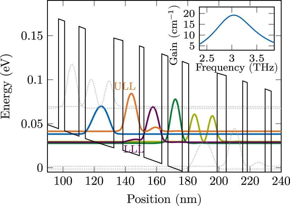
Conduction band profile and probability densities of the used QCL active region at an applied bias of 6 kV cm−1. The inset shows the power gain obtained from EMC simulations at this bias.
When we apply such an advanced active region model to a pristine cavity of length 2.9 mm, we obtain an unlocked state, as visible in Figure 6. The time trace of the outcoupled intensity is visualized in (a), where the upper and lower blue lines refer to the intensity maxima and minima of each round trip, respectively. The gray shaded area consequently indicates the intensity modulations. Considering a typical cross-sectional area of 1,000 µm2 for THz QCLs, the outcoupled power here is
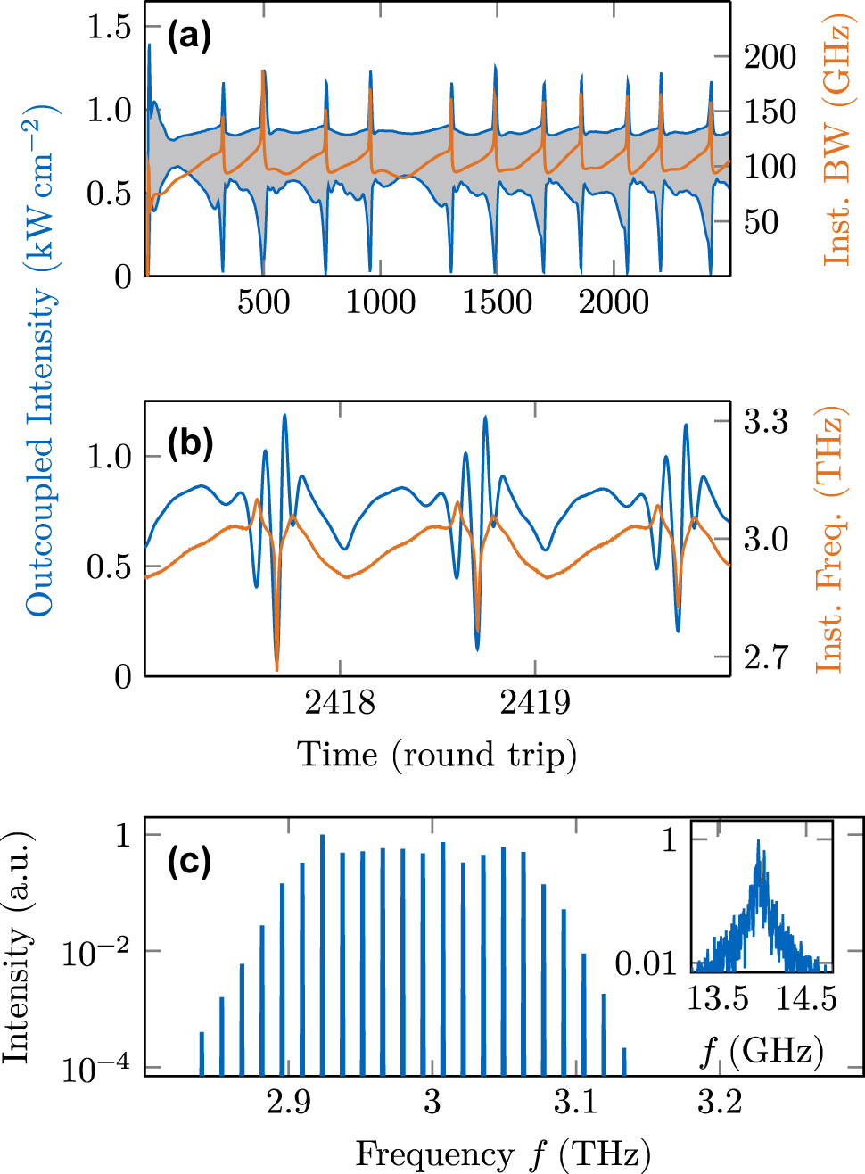
Dynamical simulation results of the active region description embedded in a pristine cavity, showing an unlocked multimode state. (a) Intensity maxima and minima of each round trip (blue) and instantaneous bandwidth (orange). (b) Intensity and instantaneous frequency over three round trips. (c) Spectrum and beatnote.
3.2 Phase locking by dispersion engineering
In the following, we apply a GTI for compensation of the excessive internal GVD imposed by the gain medium [24], to achieve stable operation. Furthermore, this type of resonator leads to a filtering effect at one end of the cavity as a frequency-dependent facet reflectivity is introduced.
Such a GTI can be realized by etching an air gap in the active region, as has been done in an experimental study of actively mode-locked THz QCLs [36]. We assume a gap with length L
gap = 2 µm between a large and a short waveguide part, representing the GTI. This type of setup is schematically shown in Figure 7a. As the air gap is significantly shorter than the wavelength of the center frequency in free space, we model it as a frequency-independent interface with complex reflection and transmission coefficients to account for the phase shift. The reflection coefficient from the waveguide to the air r
12 = 0.83 has been extracted from a numerical electromagnetic simulation [36], and from the air to the waveguide r
21 = −0.83. Then, we obtain from Eqs. (10) and (11) the complex reflection and transmission coefficients of the air gap as r
gap = 0.3089 − 0.4563i and t
gap = 0.6910 + 0.4678i at a center frequency of 2.96 THz. To better understand the behavior of this rather complex GTI structure, we numerically investigate its influence on a broadband Gaussian pulse by comparing it before and after interaction with the GTI. From this pump–probe type simulation, the net gain and dispersion of the system can be retrieved by comparing the spectra of the incident and reflected pulse [49]. By including the GTI into the numerical RNFD scheme as a spatially extended structure with partially reflecting and transmitting interfaces, the frequency dependence of the GVD in the relevant bandwidth is fully captured in our model. In addition to the simulation with both the GTI and the active region, we also simulate once with only the GTI and once with only the QCL gain medium. The numerical results for the GVD and spectral net gain of a setup with GTI-length L
GTI = 65 µm and a waveguide loss of 15 cm−1 are shown in Figure 7b and c, respectively. We observe that the GTI significantly reduces the GVD introduced by the five-level QCL gain medium in the relevant frequency range of

Dispersion engineering using a Gires–Tournois interferometer. (a) Illustration of a THz QCL with a GTI, probed by a THz pulse for its characterization. (b) Group velocity dispersions of a GTI with 65 µm length and 2 µm gap, of the gain medium, and their sum. (c) Net gain properties of the investigated device with and without GTI compared to the overall loss (waveguide + facets) in the presence of the GTI.
Equally important for the laser operation is the influence of the GTI on the overall net gain. While the air gap is in first approximation frequency-independent, the length of the short active region section is in the range of 2–3 wavelengths and thus introduces a strong frequency dependence. This is very well visible in Figure 7c. In the presence of the GTI, but without a gain medium (black line), the system shows largely increased loss at
In the here described case, the dispersion reduction and filtering effects yield phase-locked multimode operation, as confirmed by a long-term simulation including the GTI and an unchanged active region model. The results are shown in Figure 8. In (a), we observe that the intensity maxima and minima are stable over many round trips and the bandwidth remains constant with time. The transient behavior occurring in the first
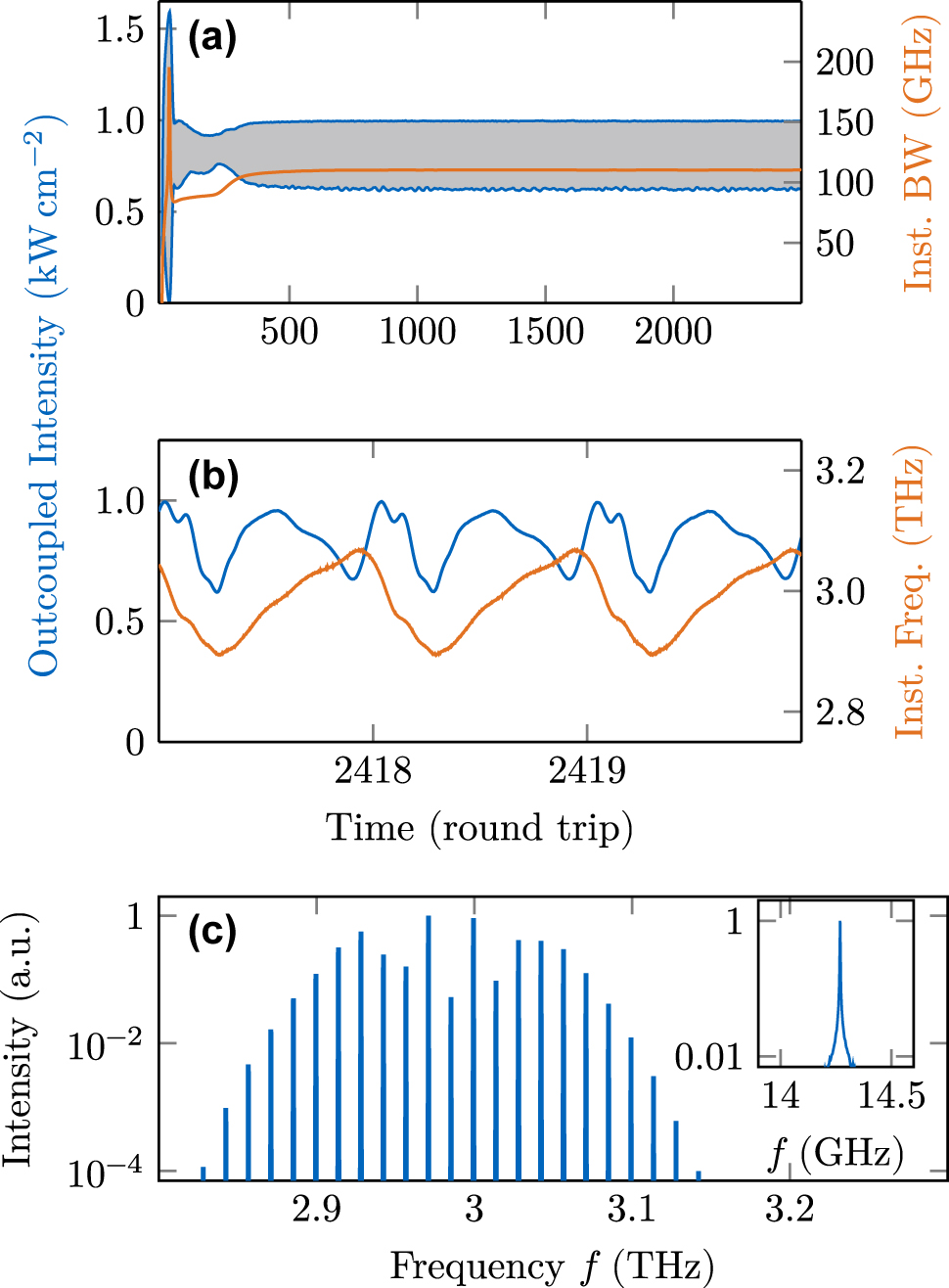
Dynamical simulation results in a cavity engineered with a Gires–Tournois interferometer. (a) Intensity and bandwidth over 2500 round trips. (b) Intensity and instantaneous frequency over three round trips. (c) Optical spectrum and beatnote.
3.3 Phase locking by field enhancement
In the previous subsection, we discussed the possibility that cavity engineering regarding GVD and frequency-dependent loss can stabilize an unlocked multimode operation of a THz QCL into an optical frequency comb. Thereby, dispersion engineering affects both the amplitude and phase of the field, according to Eq. (2). In contrast, a tapered waveguide acts on the intensity only. Therefore, the question arises whether this is sufficient to lock the modes and, if so, how the taper interacts with the gain medium to stabilize comb operation.
3.3.1 Single tapered cavity
The first question can be straightforwardly tackled by our numerical simulation approach, where we take a cavity with the layout as shown in Figure 4a. We choose the length of both tapers to be 300 µm and the narrow section in between 600 µm, while the two broad outer sections are both 900 µm, such that the overall cavity length adds up to 3 mm. The tapering factors are obtained from Eq. (12) as α
1 = 0.25 and α
2 = 4, respectively. As discussed in Section 3.1, an untapered device with the given active region model and waveguide length results in an unlocked state. When performing the simulation including the described taper, an optical frequency comb is obtained, characterized by the noise quantifiers σ
P = 0.0080 mW and σ
ΔΦ = 0.0065 rad, and a beatnote linewidth below our numerical resolution limit
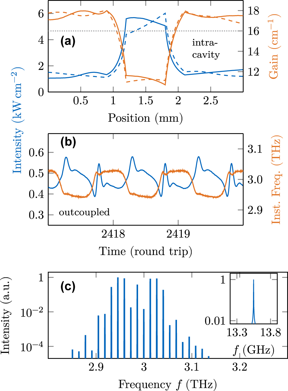
Dynamical simulation results in a cavity engineered by a tapered section. (a) Intracavity intensity (blue) and gain (orange). Solid lines refer to right-traveling properties, and dashed lines to left-traveling ones. (b) Outcoupled intensity and instantaneous frequency over three round trips. (c) Optical spectrum and beatnote.
In the time trace of this simulation, plotted in Figure 9b, two dominant observations can be made. First, the intensity modulation amplitude is with
3.3.2 Double tapered cavity
Finally, we apply our model to an experimentally realized device [37]. To this end, we extend the previously used tapered device with another taper section of the same dimensions. The section length of the first and last broad regions is reduced to 450 µm, such that the overall length of the device is
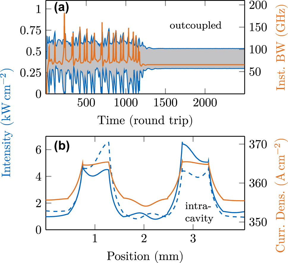
Dynamical simulation results in a cavity engineered by two tapered sections for a 2nd order HFC. (a) Outcoupled intensity maxima and minima (blue) and bandwidth (orange) over many round trips. (b) Intracavity intensity (blue) and current density (orange). The solid blue line refers to the right-traveling field, and the dashed line to the left-traveling one.
In experiments with such a double tapered QCL device, multiple HFCs with varying mode spacing were found, but so far not numerically modeled, to the best of our knowledge [37]. Indeed, the simulation shown in Figure 10 results in a 2FSR HFC. Due to the symmetry of the double tapered cavity and the introduced reflections, this behavior is not surprising, as symmetrically engineered cavities support HFC operation [31]. For further investigation, we use the EMC approach to extract several active region descriptions at different biases and temperatures from the QCL design given in Figure 5. We obtain mode spacings that range from a dense comb to the 6th harmonic state with the same cavity properties, as also observed in experiment [37]. Exemplary spectra are depicted in Figure 11a–c, with the lowest present beatnote of the modes given in the according inset. The 6FSR state reaches the maximum bandwidth with modes in a range of
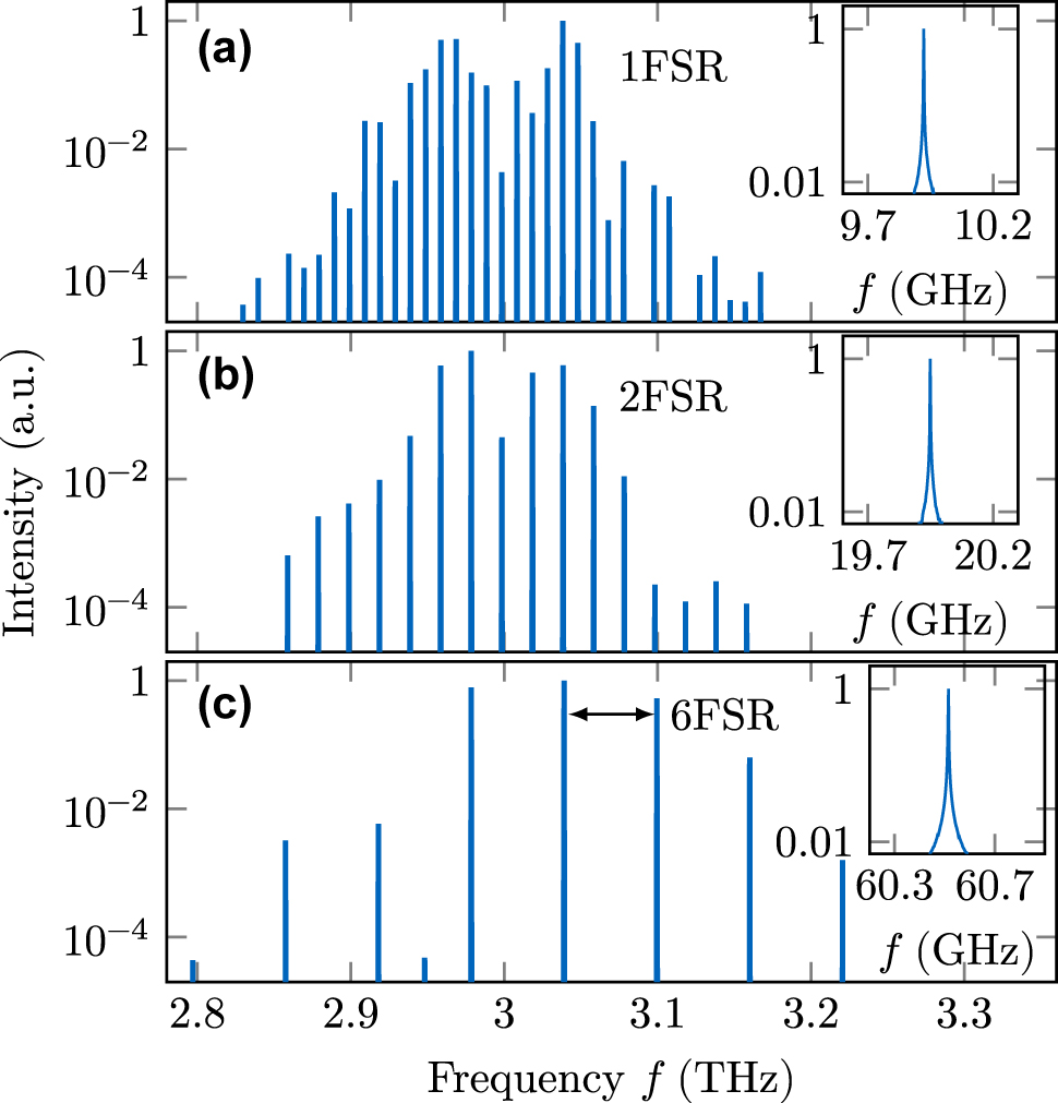
Exemplary output spectra of the double tapered cavity for different biases and temperatures. Harmonic frequency combs of different order can arise for the same cavity, with (a) and (b) even resulting from identical simulation parameters.
The time traces of intensity and instantaneous frequency associated with the spectra of Figure 11 are plotted in Figure 12a–c over three round trip times t rt. In all cases, hybrid amplitude and frequency modulation is observed, typical for THz QCLs [57], [58]. The periodicity is reduced according to the inverse of the mode spacing. In the fundamental case of Figure 12a, the instantaneous frequency chirps from its minimum to the maximum value with significant wiggles and then rapidly back to the minimum, in agreement with the experimental observations [37]. The amplitude fluctuations become more regular with increasing repetition frequency of the modulation in higher harmonic combs. Thereby, the instantaneous frequency in Figure 12c chirps nearly linearly between the two extremas, with approximately equal up- and down-chirp times.
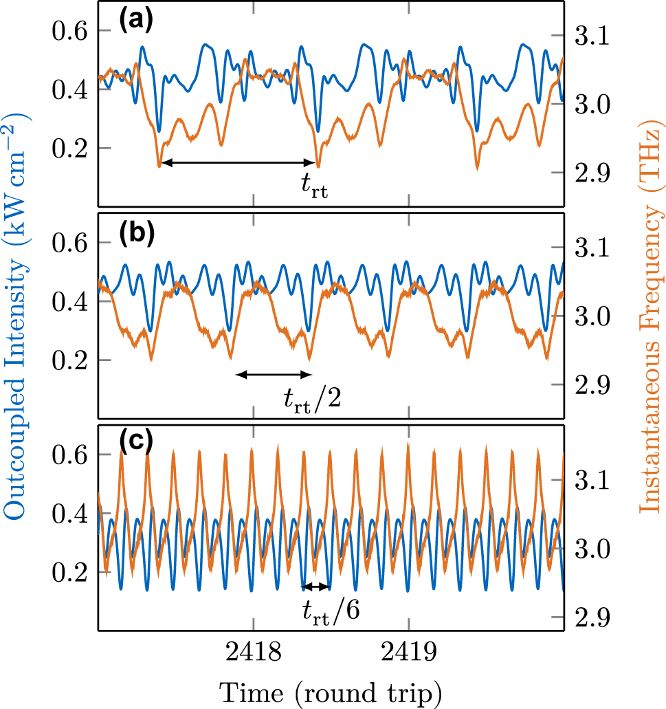
Time traces and instantaneous frequencies of the different comb states shown in Figure 11.
The outcoupled power is with 3–5 mW slightly higher than found experimentally when assuming an active region cross-section of 1,000 µm2, which might be explained by the THz detection efficiency and the large opening angle of the radiation. The current density varies from 110 A cm−2 to 360 A cm−2. These values are a little lower than the measured range (≈ 200 A cm−2 to 400 A cm−2) [37], so the electric current is more efficiently converted to an optical field in the simulation than in the real device. Since parasitic effects, such as leakage current, are neglected in the model, this slight underestimation is well explainable.
The fact that multiple harmonic comb operations are highly stable in a cavity with a single symmetry in propagation direction is somewhat unexpected, given the fact that custom engineered HFCs of previous work closely followed the cavity structure [29], [31]. A reasoning might include the dynamic interplay between the active region properties, such as the gain bandwidth and recovery time, or tunneling energies, with the cavity dimensions. A more detailed analysis exceeds the scope of this paper, but will be part of our future work.
4 Summary and conclusion
In summary, we have presented a dynamical model for QCLs that accounts for reflection and transmission processes, including propagation in several media of varying refractive indices. The numerical implementation, considering phase correction factors and varying grid spacing, is validated against the analytical reflectance formula for a double-material interface. Furthermore, we have derived a model to include tapered waveguide sections in the form of an intensity gain or loss, depending on the shape of the taper and the field propagation direction. To investigate the impact of cavity engineering on THz QCL operation, we obtain an active region description by self-consistently solving the Schrödinger–Poisson and Monte-Carlo rate equations for an experimentally realized semiconductor heterostructure. Simulating this structure in a pristine cavity yields an unlocked multimode state and forms the starting point of our cavity engineering approach. At first, we show that including a GTI, which can be monolithically integrated into the waveguide, compensates for excessive GVD of the active region and thus enables frequency comb formation. Then, it is discussed that introducing a single tapered section to an otherwise pristine ridge waveguide can also have a beneficial influence on phase locking due to its peculiar interplay with the gain medium. Our simulations show that HFC formation in double-tapered waveguides is not necessarily linked to the symmetries of the cavity. We have reproduced the harmonic state switching observed experimentally, making these exotic frequency comb types more accessible. An advantage of our full numerical multilevel model is that it can be used for a wide range of QCL active region designs, including mid-infrared devices [30], [59]. Our future work will aim to better understand the occurrence of HFCs and investigate the influence of GTIs and tapered sections on actively mode-locked QCLs. Finally, we conclude that engineering the cavity of a THz QCL can enable multimode phase locking and frequency comb formation and even be used to shape the coherent field properties.
Funding source: Deutsche Forschungsgemeinschaft
Award Identifier / Grant number: 491801597
-
Research funding: The authors acknowledge financial support by the European Union’s QuantERA II [G.A. n. 101017733] – QATACOMB Project “Quantum correlations in terahertz QCL combs” (Funding organization DFG – Germany [Project n. 491801597]).
-
Author contributions: LS: conceptualization, formal analysis, investigation, methodology, software, visualization, writing original draft, writing review & editing. MAS, MR, NP: investigation, validation, methodology, software, writing review & editing. MH: data curation, resources, visualization, software, writing review & editing. CJ: funding acquisition, project administration, supervision, software, writing review & editing. All authors have accepted responsibility for the entire content of this manuscript and consented to its submission to the journal, reviewed all the results and approved the final version of the manuscript.
-
Conflict of interest: Authors state no conflicts of interest.
-
Data availability: The datasets generated and/or analyzed during the current study are available from the corresponding author upon reasonable request.
Derivation of tapering loss function
We consider a tapered region between x 1 and x 2. Assuming an adiabatically changing transverse mode profile along the taper, we show that in the 1D model the associated intensity change can be equivalently modeled by an effective loss coefficient a t. We describe the width ratio along the tapered section between x 1 and x 2 by an arbitrary function
Multiplying Eq. (2) with
Introducing the retarded time variables t R = t ∓ x/v g, x R = x yields
On the other hand, from Eq. (A.1) we obtain the taper-induced change in intensity
Thus, the taper is represented in the 1D model as an effective loss coefficient in one direction and an effective gain coefficient in the other direction. For an adiabatic linear taper, which widens respectively narrows the waveguide by a factor
References
[1] A. Leitenstorfer, et al.., “The 2023 terahertz science and technology roadmap,” J. Phys. D: Appl. Phys., vol. 56, no. 22, p. 223001, 2023, https://doi.org/10.1088/1361-6463/acbe4c.Search in Google Scholar
[2] J. Faist, F. Capasso, D. L. Sivco, C. Sirtori, A. L. Hutchinson, and A. Y. Cho, “Quantum cascade laser,” Science, vol. 264, no. 5158, pp. 553–556, 1994. https://doi.org/10.1126/science.264.5158.553.Search in Google Scholar PubMed
[3] R. Köhler, et al.., “Terahertz semiconductor-heterostructure laser,” Nature, vol. 417, no. 6885, pp. 156–159, 2002, https://doi.org/10.1038/417156a.Search in Google Scholar PubMed
[4] A. Hugi, G. Villares, S. Blaser, H. C. Liu, and J. Faist, “Mid-infrared frequency comb based on a quantum cascade laser,” Nature, vol. 492, no. 7428, pp. 229–233, 2012, https://doi.org/10.1038/nature11620.Search in Google Scholar PubMed
[5] D. Burghoff, et al.., “Terahertz laser frequency combs,” Nat. Photon., vol. 8, no. 6, pp. 462–467, 2014, https://doi.org/10.1038/nphoton.2014.85.Search in Google Scholar
[6] J. Faist, et al.., “Quantum cascade laser frequency combs,” Nanophotonics, vol. 5, no. 2, pp. 272–291, 2016, https://doi.org/10.1515/nanoph-2016-0015.Search in Google Scholar
[7] S. Barbieri, et al.., “Coherent sampling of active mode-locked terahertz quantum cascade lasers and frequency synthesis,” Nat. Photon., vol. 5, no. 5, pp. 306–313, 2011. https://doi.org/10.1038/nphoton.2011.49.Search in Google Scholar
[8] E. Riccardi, et al.., “Short pulse generation from a graphene-coupled passively mode-locked terahertz laser,” Nat. Photon., vol. 17, no. 7, pp. 607–614, 2023. https://doi.org/10.1038/s41566-023-01195-z.Search in Google Scholar
[9] J. B. Khurgin, Y. Dikmelik, A. Hugi, and J. Faist, “Coherent frequency combs produced by self frequency modulation in quantum cascade lasers,” Appl. Phys. Lett., vol. 104, no. 8, p. 081118, 2014, https://doi.org/10.1063/1.4866868.Search in Google Scholar
[10] M. Singleton, P. Jouy, M. Beck, and J. Faist, “Evidence of linear chirp in mid-infrared quantum cascade lasers,” Optica, vol. 5, no. 8, pp. 948–953, 2018. https://doi.org/10.1364/optica.5.000948.Search in Google Scholar
[11] D. Kazakov, et al.., “Self-starting harmonic frequency comb generation in a quantum cascade laser,” Nat. Photon., vol. 11, no. 12, pp. 789–792, 2017. https://doi.org/10.1038/s41566-017-0026-y.Search in Google Scholar
[12] M. Piccardo, et al.., “The harmonic state of quantum cascade lasers: origin, control, and prospective applications,” Opt. Express, vol. 26, no. 8, pp. 9464–9483, 2018, https://doi.org/10.1364/oe.26.009464.Search in Google Scholar PubMed
[13] A. Forrer, Y. Wang, M. Beck, A. Belyanin, J. Faist, and G. Scalari, “Self-starting harmonic comb emission in THz quantum cascade lasers,” Appl. Phys. Lett., vol. 118, no. 13, p. 131112, 2021, https://doi.org/10.1063/5.0041339.Search in Google Scholar
[14] A. Khalatpour, M. C. Tam, S. J. Addamane, J. Reno, Z. Wasilewski, and Q. Hu, “Enhanced operating temperature in terahertz quantum cascade lasers based on direct phonon depopulation,” Appl. Phys. Lett., vol. 122, no. 16, p. 161101, 2023, https://doi.org/10.1063/5.0144705.Search in Google Scholar
[15] U. Senica, et al.., “Continuously tunable coherent pulse generation in semiconductor lasers,” arXiv preprint arXiv:2411.11210, 2024, https://doi.org/10.48550/arXiv.2411.11210.Search in Google Scholar
[16] Y. Wu, M. A. Schreiber, A. D. Kim, S. J. Addamane, C. Jirauschek, and B. S. Williams, “Harmonic and subharmonic RF injection locking of THz metasurface quantum-cascade vecsel,” ACS Photonics, vol. 11, no. 11, pp. 4515–4523, 2024, https://doi.org/10.1021/acsphotonics.4c00608.Search in Google Scholar PubMed PubMed Central
[17] V. Pistore, et al.., “Self-induced phase locking of terahertz frequency combs in a phase-sensitive hyperspectral near-field nanoscope,” Adv. Sci., vol. 9, no. 28, p. 2200410, 2022, https://doi.org/10.1002/advs.202200410.Search in Google Scholar PubMed PubMed Central
[18] L. Allen and J. H. Eberly, Optical Resonance and Two-Level Atoms, New York, Dover Publications, 1987.Search in Google Scholar
[19] C. Y. Wang, et al.., “Coherent instabilities in a semiconductor laser with fast gain recovery,” Phys. Rev. A, vol. 75, no. 3, p. 031802(R), 2007. https://doi.org/10.1103/physreva.75.031802.Search in Google Scholar
[20] A. Gordon, et al.., “Multimode regimes in quantum cascade lasers: From coherent instabilities to spatial hole burning,” Phys. Rev. A, vol. 77, no. 5, p. 053804, 2008. https://doi.org/10.1103/physreva.77.053804.Search in Google Scholar
[21] C. Jirauschek and T. Kubis, “Modeling techniques for quantum cascade lasers,” Appl. Phys. Rev., vol. 1, no. 1, p. 011307, 2014, https://doi.org/10.1063/1.4863665.Search in Google Scholar
[22] A. Wacker, M. Lindskog, and D. O. Winge, “Nonequilibrium Green’s function model for simulation of quantum cascade laser devices under operating conditions,” IEEE J. Sel. Top. Quantum Electron., vol. 19, no. 5, p. 1200611, 2013, https://doi.org/10.1109/jstqe.2013.2239613.Search in Google Scholar
[23] M. Riesch and C. Jirauschek, “mbsolve: An open-source solver tool for the Maxwell-Bloch equations,” Comput. Phys. Commun., vol. 268, p. 108097, 2021. https://doi.org/10.1016/j.cpc.2021.108097.Search in Google Scholar
[24] C. Jirauschek, M. Riesch, and P. Tzenov, “Optoelectronic device simulations based on macroscopic Maxwell-Bloch equations,” Adv. Theory Simul., vol. 2, no. 8, p. 1900018, 2019, https://doi.org/10.1002/adts.201900018.Search in Google Scholar
[25] N. Opačak and B. Schwarz, “Theory of frequency-modulated combs in lasers with spatial hole burning, dispersion, and Kerr nonlinearity,” Phys. Rev. Lett., vol. 123, no. 24, p. 243902, 2019, https://doi.org/10.1103/physrevlett.123.243902.Search in Google Scholar
[26] D. Burghoff, “Unraveling the origin of frequency modulated combs using active cavity mean-field theory,” Optica, vol. 7, no. 12, pp. 1781–1787, 2020, https://doi.org/10.1364/optica.408917.Search in Google Scholar
[27] C. Silvestri, X. Qi, T. Taimre, and A. D. Rakić, “Frequency combs induced by optical feedback and harmonic order tunability in quantum cascade lasers,” APL Photonics, vol. 8, no. 11, p. 116102, 2023, https://doi.org/10.1063/5.0164597.Search in Google Scholar
[28] C. Silvestri, M. Brambilla, P. Bardella, and L. L. Columbo, “Unified theory for frequency combs in ring and Fabry–Perot quantum cascade lasers: An order-parameter equation approach,” APL Photonics, vol. 9, no. 7, p. 076119, 2024. https://doi.org/10.1063/5.0213323.Search in Google Scholar
[29] D. Kazakov, et al.., “Defect-engineered ring laser harmonic frequency combs,” Optica, vol. 8, no. 10, pp. 1277–1280, 2021, https://doi.org/10.1364/optica.430896.Search in Google Scholar
[30] L. Seitner, et al.., “Backscattering-induced dissipative solitons in ring quantum cascade lasers,” Phys. Rev. Lett., vol. 132, no. 4, p. 043805, 2024. https://doi.org/10.1103/physrevlett.132.043805.Search in Google Scholar
[31] E. Riccardi, et al.., “Sculpting harmonic comb states in terahertz quantum cascade lasers by controlled engineering,” Optica, vol. 11, no. 3, pp. 412–419, 2024, https://doi.org/10.1364/optica.509929.Search in Google Scholar
[32] C. Jirauschek, “Theory of hybrid microwave–photonic quantum devices,” Laser Photonics Rev., vol. 17, no. 12, p. 2300461, 2023. https://doi.org/10.1002/lpor.202300461.Search in Google Scholar
[33] L. Seitner, J. Popp, M. Haider, S. S. Dhillon, M. S. Vitiello, and C. Jirauschek, “Theoretical model of passive mode-locking in terahertz quantum cascade lasers with distributed saturable absorbers,” Nanophotonics, vol. 13, no. 10, pp. 1823–1834, 2024, https://doi.org/10.1515/nanoph-2023-0657.Search in Google Scholar PubMed PubMed Central
[34] J. Popp, et al.., “Self-consistent simulations of intracavity terahertz comb difference frequency generation by mid-infrared quantum cascade lasers,” J. Appl. Phys., vol. 133, no. 23, p. 233103, 2023, https://doi.org/10.1063/5.0151036.Search in Google Scholar
[35] G. Villares, et al.., “Dispersion engineering of quantum cascade laser frequency combs,” Optica, vol. 3, no. 3, pp. 252–258, 2016, https://doi.org/10.1364/optica.3.000252.Search in Google Scholar
[36] F. Wang, et al.., “Short terahertz pulse generation from a dispersion compensated modelocked semiconductor laser,” Laser Photonics Rev., vol. 11, no. 4, p. 1700013, 2017, https://doi.org/10.1002/lpor.201700013.Search in Google Scholar
[37] U. Senica, et al.., “Frequency-modulated combs via field-enhancing tapered waveguides,” Laser Photonics Rev., vol. 17, no. 12, p. 2300472, 2023, https://doi.org/10.1002/lpor.202300472.Search in Google Scholar
[38] C. Jirauschek, “Dynamic modeling of quantum optoelectronic devices,” in 2023 IEEE Nanotechnology Materials and Devices Conference (NMDC), Paestum, Italy, IEEE, 2023, pp. 608–612.10.1109/NMDC57951.2023.10344140Search in Google Scholar
[39] H. Risken and K. Nummedal, “Self-pulsing in lasers,” J. Appl. Phys., vol. 39, no. 10, pp. 4662–4672, 1968, https://doi.org/10.1063/1.1655817.Search in Google Scholar
[40] C. Jirauschek, “Modeling of microstrip quantum cascade lasers,” in 2022 Photonics & Electromagnetics Research Symposium (PIERS), Hangzhou, China, IEEE, 2022, pp. 919–923.10.1109/PIERS55526.2022.9792741Search in Google Scholar
[41] B. S. Williams, “Terahertz quantum-cascade lasers,” Nat. Photon., vol. 1, no. 9, pp. 517–525, 2007, https://doi.org/10.1038/nphoton.2007.166.Search in Google Scholar
[42] B. Schwarz, et al.., “Monolithically integrated mid-infrared lab-on-a-chip using plasmonics and quantum cascade structures,” Nat. Commun., vol. 5, no. 1, p. 4085, 2014, https://doi.org/10.1038/ncomms5085.Search in Google Scholar PubMed PubMed Central
[43] U. Senica, et al.., “Planarized THz quantum cascade lasers for broadband coherent photonics,” Light Sci. Appl., vol. 11, p. 347, 2022, https://doi.org/10.1038/s41377-022-01058-2.Search in Google Scholar PubMed PubMed Central
[44] M. Born and E. Wolf, Principles of Optics: 60th Anniversary Edition, 7th ed. Cambridge, UK, Cambridge University Press, 2019.10.1017/9781108769914Search in Google Scholar
[45] M. Jaidl, et al.., “Comb operation in terahertz quantum cascade ring lasers,” Optica, vol. 8, no. 6, pp. 780–787, 2021, https://doi.org/10.1364/optica.420674.Search in Google Scholar
[46] F. P. Mezzapesa, et al.., “Tunable and compact dispersion compensation of broadband THz quantum cascade laser frequency combs,” Opt. Express, vol. 27, no. 15, pp. 20 231–20 240, 2019, https://doi.org/10.1364/oe.27.020231.Search in Google Scholar
[47] F. P. Mezzapesa, et al.., “Terahertz frequency combs exploiting an on-chip, solution-processed, graphene-quantum cascade laser coupled-cavity,” ACS Photonics, vol. 7, no. 12, pp. 3489–3498, 2020, https://doi.org/10.1021/acsphotonics.0c01523.Search in Google Scholar PubMed PubMed Central
[48] M. A. Justo Guerrero, O. Arif, L. Sorba, and M. S. Vitiello, “Harmonic quantum cascade laser terahertz frequency combs enabled by multilayer graphene top-cavity scatters,” Nanophotonics, vol. 13, no. 10, pp. 1835–1841, 2024, https://doi.org/10.1515/nanoph-2023-0912.Search in Google Scholar PubMed PubMed Central
[49] P. Tzenov, D. Burghoff, Q. Hu, and C. Jirauschek, “Time domain modeling of terahertz quantum cascade lasers for frequency comb generation,” Opt. Express, vol. 24, no. 20, pp. 23 232–23 247, 2016, https://doi.org/10.1364/oe.24.023232.Search in Google Scholar
[50] A. Forrer, et al.., “Photon-driven broadband emission and frequency comb RF injection locking in THz quantum cascade lasers,” ACS Photonics, vol. 7, no. 3, pp. 784–791, 2020, https://doi.org/10.1021/acsphotonics.9b01629.Search in Google Scholar
[51] V. Rindert, E. Önder, and A. Wacker, “Analysis of high-performing terahertz quantum cascade lasers,” Phys. Rev. Appl., vol. 18, no. 4, p. L041001, 2022.10.1103/PhysRevApplied.18.L041001Search in Google Scholar
[52] C. Jirauschek, “Density matrix Monte Carlo modeling of quantum cascade lasers,” J. Appl. Phys., vol. 122, no. 13, p. 133105, 2017, https://doi.org/10.1063/1.5005618.Search in Google Scholar
[53] C. Silvestri, L. L. Columbo, M. Brambilla, and M. Gioannini, “Coherent multi-mode dynamics in a quantum cascade laser: amplitude- and frequency-modulated optical frequency combs,” Opt. Express, vol. 28, no. 16, pp. 23 846–23 861, 2020, https://doi.org/10.1364/oe.396481.Search in Google Scholar PubMed
[54] M. Roy, Z. Xiao, C. Dong, S. Addamane, and D. Burghoff, “Fundamental bandwidth limits and shaping of frequency-modulated combs,” Optica, vol. 11, no. 8, pp. 1094–1102, 2024, https://doi.org/10.1364/optica.529119.Search in Google Scholar
[55] J. Popp, et al.., “Modeling of fluctuations in dynamical optoelectronic device simulations within a Maxwell-density matrix Langevin approach,” APL Quantum, vol. 1, no. 1, p. 016109, 2024. https://doi.org/10.1063/5.0183828.Search in Google Scholar
[56] T. S. Mansuripur, et al.., “Single-mode instability in standing-wave lasers: The quantum cascade laser as a self-pumped parametric oscillator,” Phys. Rev. A, vol. 94, no. 6, p. 063807, 2016. https://doi.org/10.1103/physreva.94.063807.Search in Google Scholar
[57] D. Burghoff, Y. Yang, D. J. Hayton, J.-R. Gao, J. L. Reno, and Q. Hu, “Evaluating the coherence and time-domain profile of quantum cascade laser frequency combs,” Opt. Express, vol. 23, no. 2, pp. 1190–1202, 2015, https://doi.org/10.1364/oe.23.001190.Search in Google Scholar
[58] F. Cappelli, et al.., “Retrieval of phase relation and emission profile of quantum cascade laser frequency combs,” Nat. Photon., vol. 13, no. 8, pp. 562–568, 2019, https://doi.org/10.1038/s41566-019-0451-1.Search in Google Scholar
[59] C. Jirauschek, “Effective discrete-level density matrix model for unipolar quantum optoelectronic devices,” Nanophotonics, 2025, https://doi.org/10.1515/nanoph-2024-0766.Search in Google Scholar PubMed PubMed Central
[60] G. Bendelli, K. Komori, and S. Arai, “Gain saturation and propagation characteristics of index-guided tapered-waveguide traveling-wave semiconductor laser amplifiers (TTW-SLA’s),” IEEE J. Quantum Electron., vol. 28, no. 2, pp. 447–458, 1992, https://doi.org/10.1109/3.123272.Search in Google Scholar
© 2025 the author(s), published by De Gruyter, Berlin/Boston
This work is licensed under the Creative Commons Attribution 4.0 International License.
Articles in the same Issue
- Frontmatter
- Editorial
- Quantum cascade laser: 30 years of discoveries
- Reviews
- Surface-emitting ring quantum cascade lasers
- From far-infrared detectors to THz QCLs
- Letter
- Mid-infrared wavelength multiplexers on an InP platform
- Research Articles
- Micro-mirror aided mid-infrared plasmonic beam combiner monolithically integrated with quantum cascade lasers and detectors
- Hybrid LiDAR–radar at 9 μm wavelength with unipolar quantum optoelectronic devices
- Compact, thermoelectrically cooled surface emitting THz QCLs operating in an HHL housing
- Extended spectral response of cavity-based terahertz photoconductive antennas and coherent detection of quantum cascade lasers
- High Q-contrast terahertz quantum cascade laser via bandgap-confined bound state in the continuum
- Effective discrete-level density matrix model for unipolar quantum optoelectronic devices
- Solitons in ultrafast semiconductor lasers with saturable absorber
- Aspects of cavity engineering in THz quantum cascade laser frequency combs
- The theory of the quantum walk comb laser