Automated assessment of immunofixations with deep neural networks
-
Christian Thiemann


Abstract
Objectives
The reliable evaluation of immunofixation electrophoresis is part of the laboratory diagnosis of multiple myeloma. Until now, this has been done routinely by the subjective assessment of a qualified laboratory staff member. The possibility of subjective errors and relatively high costs with long staff retention are the challenges of this approach commonly used today.
Methods
Deep Convolutional Neural Networks are applied to the assessment of immunofixation images. In addition to standard monoclonal gammopathies (IgA-Kappa, IgA-Lambda, IgG-Kappa, IgG-Lambda, IgM-Kappa, and IgM-Lambda), also bi- or oligoclonal gammopathies, free chain gammopathies, non-pathological cases, and cases with no clear finding are detected. The assignment to one of these 10 classes comes with a confidence value.
Results
On a test data set with over 4,000 images, approximately 25% of the cases are sorted out as inconclusive or due to low confidence for subsequent manual evaluation. On the remaining 75%, about 3,000 cases, not even one is classified as falsely positive, and only one as falsely negative. The remaining few deviations of the automated assessment from the classifications assigned manually by experts are borderline cases or can be explained otherwise. As a software running on a standard desktop computer, the Deep Convolutional Neural Network needs less than a second for the assessment of an immunofixation image.
Conclusions
Assisting the laboratory expert in the assessment of immunofixation images can be a useful addition to laboratory diagnostics. However, the decision-making authority should always remain with the physician responsible for the findings.
Introduction
Artificial intelligence (AI) has found many applications in medicine. Especially in medical imaging, modern methods of intelligent pattern recognition can support diagnosis. Deep Convolutional Neural Networks are usually used for this purpose [1], [2], [3], [4]. The evaluation of immune fixations is also image-based and is still performed manually by experts. Therefore, it is obvious to apply Deep Convolutional Neural Networks also to the evaluation of immunofixation images.
A monoclonal gammopathy is characterized by an increased concentration of a monoclonal paraprotein secreted by an autonomously proliferating B lymphocyte or plasma cell clone [5]. Both, complete immunoglobulins of the type IgG, IgA or IgM (rarely IgD or IgE; therefore not included in standard diagnostics initially, but in step diagnostics) with the corresponding light chains κ (Kappa) or λ (Lambda) and only free light chains (so-called light chain myeloma) can be formed. Very rarely, only heavy chains are synthesized. The monoclonal paraprotein is often visible in electrophoresis as a so-called M-gradient (“M-protein”) in the γ- or β-fraction. Sensitive detection and differentiation of the underlying immunoglobulin type is achieved by immunofixation. Free light chains should also be quantitatively determined according to current guidelines. The diagnosis of multiple myeloma always includes bone marrow diagnostics by cytology (>10% monoclonal plasma cells) and flow cytometry as well as clinical chemistry parameters (calcium, creatinine; β2-Mikroglobulin) and imaging of the skeletal system (osteolysis on X-ray or computed tomography). In general, the indication for therapy is derived from the CRAB criteria: “hypercalcemia”, “renal insufficiency”, “anemia” and “bone lesions”. A single and sole assessment of immunofixation is neither suitable for the diagnosis nor for the exclusion of multiple myeloma.
In addition, detection of a monoclonal paraprotein is only an indication – not proof – of multiple myeloma or another neoplasia of B lymphocytes or plasma cells requiring treatment. Laboratory evidence alone, without clinical symptoms, indicates a monoclonal gammopathy of uncertain significance (MGUS) or smouldering myeloma.
The evaluation of immunofixation has so far been performed in the laboratory routine by eye evaluation and subjective assessment. Even if a laboratory result alone should not lead to a clinical decision, the result quality of each individual laboratory result must be high. Support in the individual evaluation by an objective AI with a final decision-making authority for the result design by the laboratory expert could therefore be a useful addition in the laboratory routine of the future.
Materials and methods
Detection of individual lanes
First, in the immunofixation image each individual lane (IgA, IgG, IgM, Kappa, and Lambda) must be identified and marked with a bounding box (Figure 1). For this the serum albumin band in the ELP lane was chosen as a reference point. Since all lanes are always in the same position relative to each other, the bounding boxes can be determined relative to the reference point. The image content within these bounding boxes are the bases for the assessment and are used as input for a Deep Neural Network.
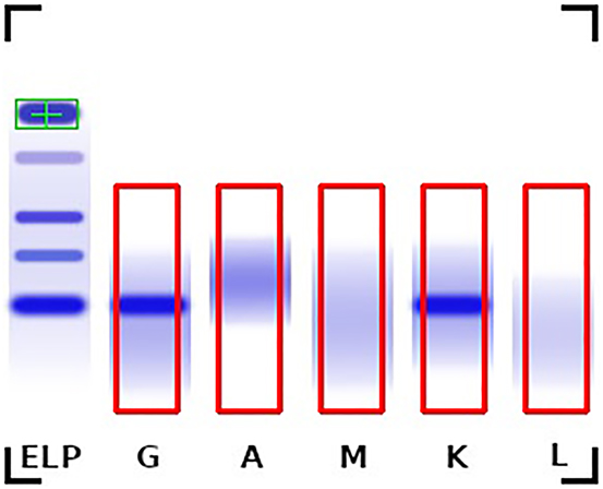
Example immunofixation image with the serum albumin reference position (green) and the bounding boxes of the individual lanes (red) shows a monoclonal gammopathy IgG type Kappa.
Automated assessment using deep neural networks
After lane detection, the five lanes of each image are passed through a Deep Neural Network system as shown in Figure 2. As Deep Neural Network a so-called ResNet18 was applied [6]. ResNet18 belongs to the class of Deep Convolutional Neural Networks. With a training dataset, described in the next section, the Neural Network has been taught to differentiate between the different types of monoclonal gammopathies as well as bi-/oligoclonal gammopathies, free chain gammopathies (FC) and non-pathological cases (Negative). Additionally, the system assigns the label “Inconclusive” in cases where no clear assessment can be made. This results in a classification problem with 10 classes.
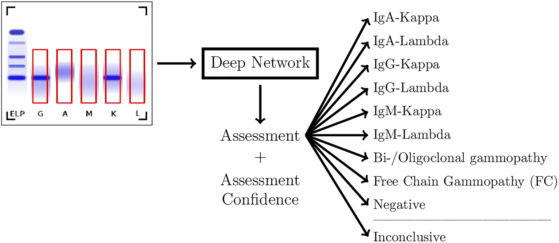
Flowchart of the assessment system.
In addition to the class label, the assessment system provides a “confidence” score for the assigned class. This score can be used to further exclude cases where the assessment is not clear enough. In this work we used a threshold of 90% for an assessment to be accepted. This value was not optimized but taken simply as “being plausible”. We will see that the exact value is not critical.
Two datasets of immunofixation images provided by LADR Laboratory Group Dr. Kramer & Colleagues were used, one for training and the other one for testing the assessment system. The images were obtained with the HYDRASYS 2 SCAN (Sebia, Lisses, France).
The patient samples came from the routine analysis of LADR Central Laboratory, a cross-sectoral large, specialized laboratory in northern Germany. 52% of the samples originated from women and 48% from men. The age composition of the patients studied was as follows: 20–29 years 3%, 30–39 years 4%, 40–49 years 7%, 50–59 years 11%, 60–69 years 20%, 70–79 years 23%, 80–89 years 25%, 90–99 years 6%. The sample pool was composed as follows regarding the initiator of the analysis: 24.3% ordered from outpatient internal medicine, 3.2% from outpatient hematology/oncology, 30.7% from outpatient general practitioners, 15.2% from outpatient neurology, and 4.5% from outpatient orthopedics. 12.6% of the orders originated from inpatient hospitals including a hospital of maximum care and specialized hematology sections as well as 9% from medical laboratories. 18% of the images originated from follow-up analyses.
Each image was assigned a label designating the finding provided for the respective image. These labels included monoclonal gammopathies (IgA-Kappa, IgA-Lambda, IgG-Kappa, IgG-Lambda, IgM-Kappa, and IgM-Lambda), bi- or oligoclonal gammopathies, free chain gammopathies, non-pathological cases. The labels were obtained from manual optical evaluation of the immunofixation gels during normal laboratory workflow.
Additionally, the datasets included cases where no clear finding was found (Inconclusive). These were cases where pathology could not be excluded with certainty despite evaluation by two experts. These evaluations also do not only include the immunofixation images, but may include previous findings, clinical information, and supplementary examinations. These background informations were not available for the AI based assessment system, since the goal was to develop an automated assessment system based only on the immunofixaton image data.
The datasets for both training and testing of the AI were generated without particular selection of samples. The samples were picked from different time intervals to ensure there is no overlap between the datasets. The dataset used to train the AI included images from late 2020 and 2021. The dataset used for testing included images from late 2019 and early 2020.
Both datasets had a roughly equal distribution of findings. As can be seen in Table 1, except for the class “free chain gammopathy” with a rather rare occurrence, in both data sets the classes more or less have the same occurrence frequency. A two-sample Kolmogorov-Smirnov test provides a statistic of 0.0082 and a p-Value of 0.9761 showing a very high correlation between the distributions of the two datasets.
Label distribution of the datasets for training and testing.
| Label | Training data | Test data |
|---|---|---|
| IgA-Kappa | 175 (1.3%) | 57 (1.3%) |
| IgA-Lambda | 112 (0.8%) | 39 (0.9%) |
| IgG-Kappa | 990 (7.0%) | 315 (7.1%) |
| IgG-Lambda | 593 (4.2%) | 208 (4.7%) |
| IgM-Kappa | 345 (2.5%) | 108 (2.4%) |
| IgM-Lambda | 124 (0.9%) | 38 (0.9%) |
| Bi-/oligoclonal gammopathy | 605 (4.3%) | 181 (4.1%) |
| Free chain gammopathy | 34 (0.2%) | 21 (0.5%) |
| Non-pathological | 9,160 (65.2%) | 2,811 (63.7%) |
| Inconclusive | 1915 (13.6%) | 638 (14.4%) |
| Total number of images | 14,053 | 4,416 |
The about three times larger set was used for training the Neural Network, and the other set was used for an independent testing.
For the development of the AI models the PyTorch [7] framework was used (Torch version 1.7.1 and Torchvision version 0.8.2). The PyTorch implementation of ResNet18 with weights pretrained on ImageNet [8] was used as a base model. For the training of the models the hyperparameters were set to an initial learning rate of 0.001, a weight decay of 0.00005, and a batch size of 64. The Adam optimizer [9] with a momentum parameter of 0.9 was used. Categorical cross entropy [10] was chosen as the loss function. Training the models for 20 epochs took approximately 20 min on a NVIDIA GeForce GTX 1070 GPU (Nvidia Corporation, Santa Clara, USA).
Results
Evaluation of the assessment system
For the evaluation of the assessment system, each image of the test dataset was passed through it. The results of this test are shown as a confusion matrix in Table 2. The analysis shows that the assessment system automatically assigns a clear label to 74.8% of the images. 25.2% of the cases are either labeled as being “inconclusive” or had a low “confidence” (less than 90%) along with its label. These images are flagged for additional manual review.
Confusion matrix of the automated assessment of the test dataset images compared to their labels.
| Label | Assessment | |||||||||||
|---|---|---|---|---|---|---|---|---|---|---|---|---|
| A–K | A–L | G–K | G–L | M–K | M–L | BO | FC | N | Inc | Total | Inconclusive or low confidence | |
| IgA-Kappa | 53 | 0 | 0 | 0 | 0 | 0 | 0 | 0 | 0 | 0 | 57 | 4 (7%) |
| IgA-Lambda | 0 | 33 | 0 | 0 | 0 | 0 | 0 | 0 | 0 | 0 | 39 | 6 (15.4%) |
| IgG-Kappa | 0 | 0 | 261 | 0 | 0 | 0 | 3 | 0 | 0 | 8 | 315 | 51 (16.2%) |
| IgG-Lambda | 0 | 0 | 0 | 160 | 0 | 0 | 4 | 1 | 0 | 14 | 208 | 43 (20.7%) |
| IgM-Kappa | 0 | 0 | 0 | 0 | 95 | 0 | 0 | 0 | 1 | 4 | 108 | 12 (11.1%) |
| IgM-Lambda | 0 | 0 | 0 | 0 | 0 | 23 | 0 | 0 | 0 | 5 | 38 | 15 (39.5%) |
| Bi-/Oligoclonal gammopathy | 2 | 1 | 10 | 11 | 5 | 0 | 82 | 0 | 0 | 12 | 181 | 70 (38.7%) |
| Free chain gammopathy | 0 | 1 | 0 | 1 | 0 | 0 | 0 | 5 | 0 | 4 | 21 | 14 (66.7%) |
| Non-pathological | 0 | 0 | 0 | 0 | 0 | 0 | 0 | 0 | 2,391 | 400 | 2,811 | 420 (14.9%) |
| Inconclusive | 1 | 0 | 8 | 2 | 1 | 3 | 2 | 0 | 145 | 424 | 638 | 476 (74.6%) |
| Total | 56 | 35 | 279 | 174 | 101 | 26 | 91 | 6 | 2,537 | 870 | 4,416 | 1,111 (25.2%) |
-
The “confidence” threshold was set to 90%. This Table includes monoclonal gammopathies (A–K through M–L), bi-/oligoclonal gammopathies (BO), free chain gammopathies (FC), non-pathological cases (N) and inconclusive cases (Inc).
From the 765 cases with labels for monoclonal gammopathies (A–K, A–L, G–K, G–L, M–K, and M–L), 131 (17.1%) were sorted out as inconclusive or low-confidence and 9 (1.2%) were assessed differently then the expert label. These include one false-negative case (n) and one case where IgG-Lambda was “wrongly” assessed as a free chain gammopathy (FC). The corresponding images are shown in Figure3A and B. In 3B one can see artefacts in the image which, of course, disturb a correct assessment. In both cases, the laboratory personnel described the monoclonal gammopathies as “hinted”. The other seven cases were assessed as bi-/oligoclonal gammopathies (BO). Manual review showed that in all of these seven cases potential additional bands might indeed hint towards bi- or oligoclonal gammopathies. Three examples are shown in Figure 3C–E.
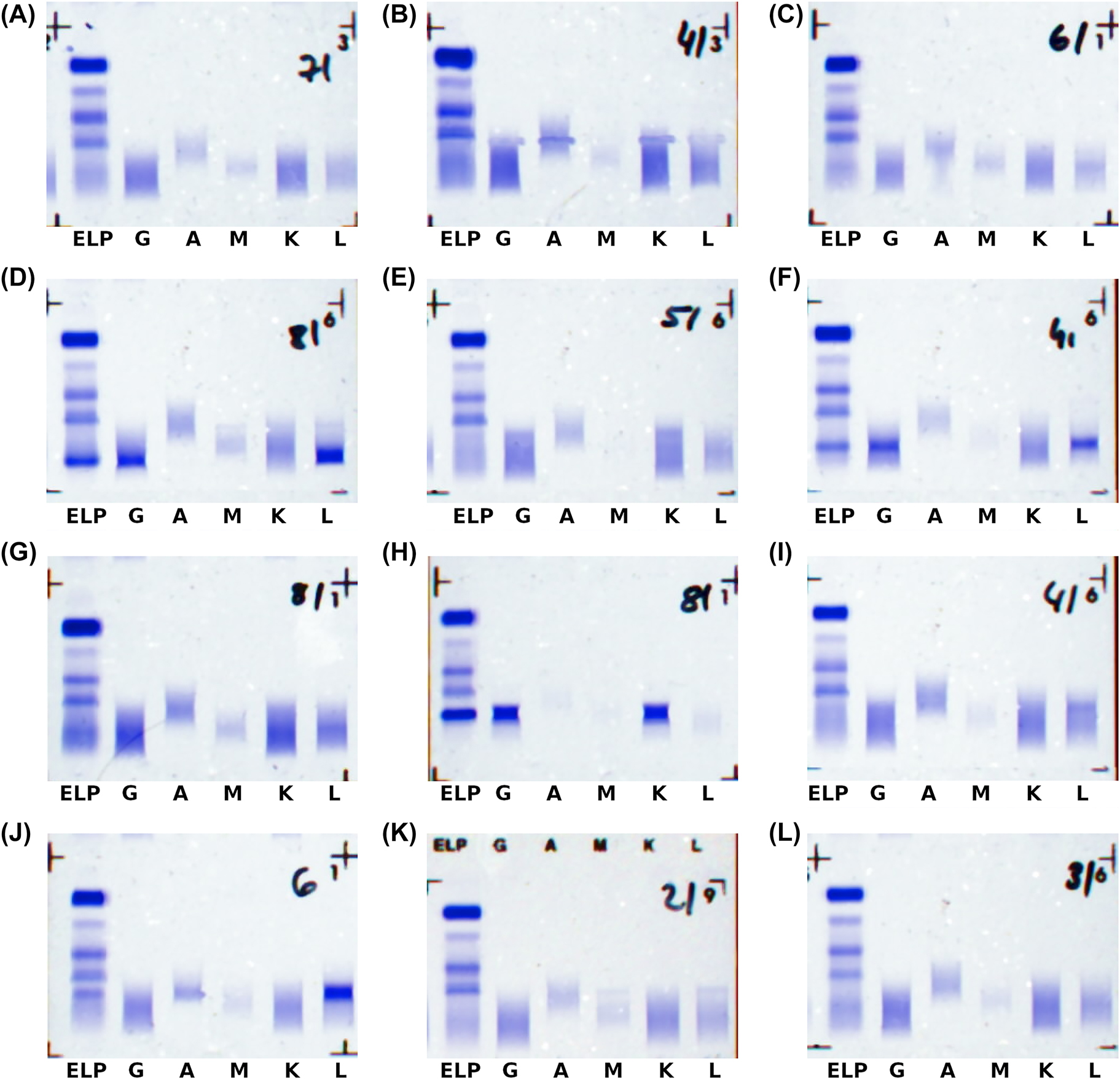
Examples where AI assessment and expert label deviate.
(A) Negative (assessment) instead of IgM-Kappa (label); (B) free chain (assessment) instead of IgG-Lambda (label), note the artefacts in the image; (C-E) bi-/oligoclonal (assessment) instead of the labels IgG-Lambda (C), IgG-Lambda (D), and IgG-Kappa (E); (F) IgG-Lambda (assessment) instead of IgG-Lambda + Lambda (label); (G) IgG-Lambda (assessment) instead of IgG-Kappa + Lambda (label); (H) IgG-Kappa (assessment) instead of biclonal IgG-Kappa (label); (I) IgG-Lambda (assessment) instead of single-lambda (label); (J) IgA-Lambda (assessment) instead of single-lambda (label); (K) IgG-Lambda (assessment) instead of inconclusive (label); (L) IgG-Kappa (assessment) instead of inconclusive (label).
From the 181 samples with the label “bi-/oligoclonal gammopathy”, 70 (38.7%) were sorted out as inconclusive or low-confidence and 29 (16.0%) were assessed as rather being monoclonal gammopathies (A–K, A–L, G–K, G–L, M–K, and M–L). 25 of them were described by the laboratory personnel as having one major monoclonal gammopathy with additional bands that are “(very) weak”, “subtle” or “hinted”. One example is shown in Figure 3F. The remaining four cases also included two edge cases where, upon manual review, no obvious label could be assigned based on the scans used in this work. These images can be seen in Figure 3G and H.
From the 21 samples with the label “free chain gammopathy”, most (66.7%) were sorted out as inconclusive or low-confidence, and 2 (10%) were assessed as rather being “complete immunoglobuline-gammopathies”. In both cases the findings describe free light chains but also mention the corresponding complete immunoglobuline paraproteins that were found by the automated assessment as potential options. Additionally, one of the samples again shows a very weak gammopathy (Figure 3I and J).
The highest confusion is given between samples that were labeled as non-pathological and samples where no clear finding could be assigned by the laboratory personnel. 400 out of 2,811 (14.2%) samples with non-pathological labels were evaluated as “Inconclusive” by the automated assessment system. Conversely, 145 out of 638 (22.7%) samples with no clear finding were assessed as non-pathological. Additionally, there were 17 cases where the system assigned a pathological label to samples with no clear finding. Examples of all these cases are shown in Figure 3K and L. Note, that no false positive assessments were made.
Overall, among the 3,143 cases where a clear label (any label except inconclusive) was assigned by both the laboratory experts and the AI (with the AI having more than 90% “confidence”), the AI assessments matched the expert labels in 98.7% of all cases.
The 1.3% deviations are the subtle cases we discussed in the previous paragraphs. For non-pathological samples there were no false positives, thus resulting in an accuracy of 100% for this subset, and from the 967 pathological cases, one (0.1%) was wrongly assessed as being negative.
With the 90% “confidence” threshold, 188 (4.3%) of the 4,416 test samples are sorted out solely because of a low “confidence”. With a 85% “confidence” threshold, it is 3.8%, and with a 95% “confidence” threshold it is 5%. With the 85% “confidence” threshold, the AI assessments match the expert labels in 98.6% of all cases, and with the 95% “confidence” threshold it is 98.9%. This shows that the choice of the “confidence” threshold in this regime is not very critical.
Discussion
Using the same image data as laboratory experts a deep learning based automated assessment system was developed. The system allows for an automation rate of approximately 75% while deviating only on very few cases. These cases are deemed borderline where no clear decision could be made based on the scans even by the experts.
Within the subset of monoclonal gammopathies there was only a single confusion, which indeed was an edge case where upon subsequent manual review no clear label could be assigned. Within the subset of all positives only one sample was wrongly predicted to be negative. Both cases were deemed to be only “hinted” gammopathies by the experts, thus making the assessment particularly difficult. Furthermore, no non-pathological sample was assessed as pathological.
For samples with bi- or oligoclonal gammopathies the reported misclassifications could also be linked to weakly defined gammopathies or edge cases where further tests would be necessary to clearly determine the presence of a bi- or oligoclonal gammopathy. For samples with free chain gammopathies an unusually high number of predictions either as “Inconclusive” or with a confidence below the threshold was observed. This is likely due to the low number of samples with this label that were available for training of the model. However, it should be emphasized that the model assesses these cases with low confidence rather than making mistakes with high confidence which is a problem commonly observed when training deep neural networks with very little data [11].
An expanded dataset including more of these rare cases might help the system to learn to differentiate them better and lead to an even higher automation rate while preserving the accuracy. Furthermore, the current dataset contains images of a comparatively low resolution. The original assessment by the experts is performed on the original immunofixation gels allowing consideration of fine details that might be lost in the images used in the automated assessment system. Implementing a scanner with a higher resolution into the system would likely further improve the performance of the automated assessment system and potentially eleviate some of the edge cases.
The assessment of immunofixations is a very time consuming and repetitive task that at the same time requires attention to detail by laboratory experts. An automated assessment system as presented in this work can support the experts and significantly speed up the workflow by simultaneously providing a constant quality and reducing the risk of erroneous assessments.
-
Research funding: None declared.
-
Author contributions: All authors have accepted responsibility for the entire content of this manuscript and approved its submission.
-
Competing interests: Authors state no conflict of interest.
-
Informed consent: Informed consent was obtained from all individuals included in this study.
-
Ethical approval: The research did not involve human subjects or animals.
References
1. Shen, L, Margolies, LR, Rothstein, JH, Fluder, E, McBride, R, Sieh, W. Deep learning to improve breast cancer detection on screening mammography. Sci Rep 2019;9:2045–322. https://doi.org/10.1038/s41598-019-48995-4.Search in Google Scholar PubMed PubMed Central
2. Kermany, DS, Goldbaum, M, Cai, W, Valentim, CCS, Liang, H, Baxter, SL, et al.. Identifying medical diagnoses and treatable diseases by image-based deep learning. Cell 2018;172:1122–31. https://doi.org/10.1016/j.cell.2018.02.010.Search in Google Scholar PubMed
3. Kiranyaz, S, Ince, T, Gabbouj, M. Real-time patient-specific ECG classification by 1-D convolutional neural networks. IEEE Trans Biomed Eng 2016;63:664–75. https://doi.org/10.1109/tbme.2015.2468589.Search in Google Scholar
4. Nasr-Esfahani, E, Samavi, S, Karimi, N, Soroushmehr, SM, Jafari, MH, Ward, K, et al.. Melanoma detection by analysis of clinical images using convolutional neural network. Annu Int Conf IEEE Eng Med Biol Soc 2016;2016:1373–6. https://doi.org/10.1109/EMBC.2016.7590963.Search in Google Scholar PubMed
5. Deutsche Krebsgesellschaft e.V. Leitlinienprogramm Onkologie [Online]. Available from: https://www.leitlinienprogramm-onkologie.de/leitlinien/multiples-myelom/ [Accessed 27 Mar 2022].Search in Google Scholar
6. He, K, Zhang, X, Ren, S, Sun, J. Deep residual learning for image recognition. IEEE Conf Comp Vis Pattern Recog 2016:770–8. https://doi.org/10.1109/cvpr.2016.90.Search in Google Scholar
7. Paszke, A, Gross, S, Massa, F, Lerer, A, Bradbury, J, Chanan, G, et al.. PyTorch: an imperative style, high-performance deep learning library. Adv Neural Inf Process Syst 2019;32:8024–35.Search in Google Scholar
8. Deng, J, Dong, W, Socher, R, Li, LJ, Li, K, Fei-Fei, L. Imagenet: a large-scale hierarchical image database. IEEE Conf Comp Vis Pattern Recog 2009:248–55. https://doi.org/10.1109/cvpr.2009.5206848.Search in Google Scholar
9. Kingma, DP, Ba, J. Adam: a method for stochastic optimization. Int Conf Learn Repres 2015.Search in Google Scholar
10. Contributors T. PyTorch. Cross entropy loss. [Online]. Available from: https://pytorch.org/docs/stable/generated/torch.nn.CrossEntropyLoss.html [Accessed 14 Mar 2022].Search in Google Scholar
11. Corbière, C, Thome, N, Bar-Hen, A, Cord, M, Pérez, P. Addressing failure prediction by learning model confidence. Conf Neural Inf Proc Syst 2019:2902–13.Search in Google Scholar
© 2022 the author(s), published by De Gruyter, Berlin/Boston
This work is licensed under the Creative Commons Attribution 4.0 International License.
Articles in the same Issue
- Frontmatter
- Original Articles
- Automated assessment of immunofixations with deep neural networks
- Non-invasive prenatal paternity testing using mini-STR-based next-generation sequencing: a pilot study
- The effect of short post-apnea time on plasma triglycerides, lipoprotein and cholesterol derived oxysterols levels
- Assessment of the diagnostic ability of RIFLE and SOFA scoring systems in comparison with protein biomarkers in acute kidney injury
- Diagnostic value of long noncoding RNA LINC01060 in gastric cancer
- Novel GLDC variants causing nonketotic hyperglycinemia in Chinese patients
- Congress Abstracts
- German Congress of Laboratory Medicine: 17th Annual Congress of the DGKL and 4th Symposium of the Biomedical Analytics of the DVTA e.V.