Energetic analysis of a non-isothermal linear energy converter operated in reverse mode (I-LEC): heat pump
-
Saul Gonzalez-Hernandez


Abstract
In this paper, we perform an energetic analysis of a non-isothermal linear energy converter operated in inverse mode (refrigerator and heat pump). This is done within the framework of linear irreversible thermodynamics (LIT), starting from the model of an inverse linear energy converter (I-LEC) proposed by S. Gonzalez et al. (S. Gonzalez-Hernandez and L.-A. Arias-Hernandez, “Thermoelectric thomson relations revisited for a linear energy converter,” J. Non-Equilibrium Thermodyn., vol. 44, no. 3, pp. 315–332, 2019). We extend this model to the case of heat pumps, considering different objective functions and performing their respective analyses. We particularly focus on the coefficient of performance (COP) of heating, ϵ H . Additionally, we propose other energetic functions that may be of interest in the analysis of heat pumps, drawing analogies with the well-known functions for refrigerators and heat engines. Finally, we present a brief description of thermoelectric phenomena, focusing primarily on the Peltier effect. A brief analysis of the results obtained in the context of thermoelectric cooling and heating is presented for a non-isothermal LEC.
1 Introduction
It is widely recognized that the advancement of energy conversion systems in recent decades has increasingly been driven by environmental concerns and, consequently, by sustainable development. In response to growing demands for reducing pollutant emissions and promoting the rational use of energy sources, stricter regulations have been implemented. This is especially true in recent times, where optimizing cooling systems for efficient use, such as in various types of supercomputing centers, has become crucial. At the same time, the depletion of energy resources and the need for greater energy efficiency have pushed for fuel consumption reduction and the development of new cooling and heating technologies. In this context, the analysis and optimization of thermoelectric cooling and heating systems emerge as a promising solution to meet, refine, and expand these requirements in the near future.
In a recent paper [1], based on Onsager’s equations [2], [3], and using Stucki’s definitions of the force quotient x and the coupling coefficient q for a 2 × 2 converter [4], a review of the classic thermocouple system was performed. The system’s operation was divided into two modes: direct (D-LEC, heat engine) and inverse (I-LEC, refrigerator) [1]. In this work, we extend the I-LEC concept to heat pumps (see Figure 1a and begin with an introduction to the I-LEC concept [1]).
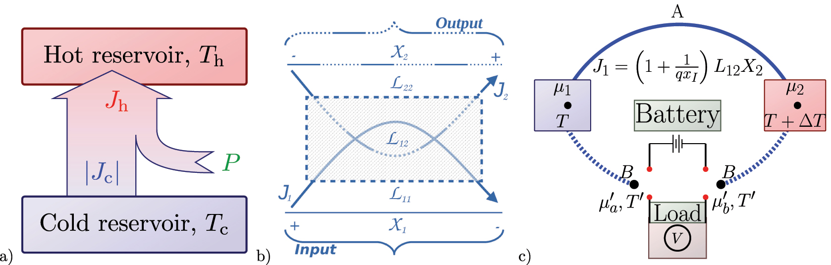
Different representations of the I-LEC. (a) Schematic representation of a heat pump. (b) Inverse Linear Energy Converter (I-LEC, like a heat pump). We have two fluxes (J
1, J
2) and two forces (X
1, X
2) and |J
2
X
2| is the power output (by temperature unit) and |J
1
X
1| is the power input (by temperature unit) of the converter. (c) Outline of a thermocouple with a variable electric current
Thermodynamic and Energy Conversion Quantities
The electrical conductivity σ
Thermal conductivity κ
Absolute thermoelectric power ɛ
Electric potential ∇μ/T
Temperature gradient −∇(1/T)
The electric charge e
The inverse force ratio x I
The coupling coefficient q
Carnot’s COP
The cooling COP ϵ = J c /P
The heating COP ϵ MH
The heating dissipation function Φ I
The production of entropy σ
Driver force X 1
Driven force X 2
The driver flux J 1 = J h
The driven flux J 2 = J c
Normalized objective functions F* = F/β
The generalized heating ecological function
The generalized heating Omega function
The generalized combined efficient power
The generalized efficient cooling power
We will begin by introducing the model of a linear energy converter (LEC), including the direct (D-LEC, heat engine) and inverse (I-LEC, heat pump and refrigerator) concepts as described [1]. For this, we consider the phenomenological Onsager equations [2], [3]:
being
the quantity (q) is called coupling coefficient, Stucki [4], and we can rewrite the Onsager’s equations as follows,
From these equations, we see that q measures the degree of coupling between the fluxes. When q → 1, the relationship between fluxes approaches a fixed mechanistic stoichiometry. On the other hand, when q → 0, the cross effects disappear, making the fluxes independent of each other. In Eq. (3), each generalized flux becomes proportional to its corresponding conjugate force through the coefficient L ii . Now, considering the system’s entropy production σ,
1.1 Direct linear energy converter (D–LEC)
Starting from the entropy production in Eq. (4), we can define two modes of operation for the system: the direct mode and the indirect mode, referred to as D-LEC and I-LEC, respectively. First, we will define the direct mode of the converter, for which we can establish the relation
Next, we can associate the first term of the entropy production with a power output (per unit of temperature) and the second term with a power input (per unit of temperature), thus constructing a steady-state Linear Energy Converter (LEC) [6], [5]. This setup represents a converter with non-zero entropy production and non-zero power output, due to its interactions with the surroundings (X k and J k , where k = 1, 2). Using the work of Caplan and Essig [6], it is possible to describe a LEC. In general, the fluxes J k governing a real system are usually highly complex and nonlinear functions of the generalized forces X k . However, the linear regime allows for a sufficiently adequate description of the phenomenon.
Now, we can use the entropy production of the LEC, given in its general form by Eq. (4), taking the heat flux as the driving flux and any other flux against a generalized force as the driven flux. For this reason, we will call this engine a “direct linear energy converter” (D-LEC). In this case, the force ratio x D is defined as:
we can write the flows J 1 and J 2 as follow,
and
Now, we make an additional hypothesis about the driver force, we will suppose that the temperature gradient is constant and of the form,
with T c and T h representing the temperatures of the “cold” and “hot” reservoirs, respectively.
1.2 Inverse energy converter (I-LEC)
Similarly, starting from the entropy production Eq. (4), we can define the Inverse Linear Energy Converter (I-LEC). To do this, we can establish the relation ∣J 2 X 2∣ > ∣J 1 X 1∣, with J 2 X 2 > 0 and J 1 X 1 < 0, according to the definitions of driven and driver fluxes [1]. The first term in the entropy production Eq. (4) can then be associated with power output, while the second term corresponds to power input per unit of temperature. Using these terms, we can build a steady-state Inverse Linear Energy Converter (I-LEC).
This converter has nonzero entropy production and nonzero power output, due to its interactions with the surroundings (i.e., forces X i and fluxes J i ). To use the force ratio x introduced by Stucki [4], we must express it for the inverse mode. In this mode, the driven flux is J 2 = J c , and the driver flux is J 1 = J h , associated with the forces X 2 and X 1 respectively. Thus, the force ratio for the I-LEC becomes:
This variable is called the inverse force ratio x I , [1], and unlike Stucki’s force ratio x, it is defined for converters operating in reverse. Therefore, −1 ≤ x I ≤ 0. Now we can write the fluxes J 1 and J 2 in terms of the inverse force ratio and the coupling coefficient as,
and
We will then extend the proposal of [1] to heat pumps, for which we take the following as the driven force:
where, T h and T c are the temperatures of the hot and cold reservoirs respectively. On the other hand, multiply the equation Eq. (9) by L 12 and substitute Eq. (2), with which we obtain,
consider the input power, P which we can define as follows [1],
replacing Eq. (10b) in, P Eq.(14), with which we obtain,
where, T
h
X
2 = −(1/ϵ
C
), and
2 Heat pump
As is well known, refrigerators, air conditioners, and heat pumps are refrigeration engines that transfer heat from a cold reservoir (J
c
) to a hotter one (J
h
) using external power P. The difference between them lies in the energy conversion objective. A refrigerator uses external work P to extract heat J
c
and move it to J
h
, with the goal of cooling the cold reservoir. In contrast, a heat pump moves J
c
using P to heat or maintain the temperature of J
h
. The objective functions that best describe the energy conversion trade-offs for these machines are different. Before analyzing heat pumps, we need to introduce the concept of normalized objective functions F* [1]. If F is a thermodynamic function obtained from linear irreversible thermodynamics (LIT), it can be normalized as F* = F/β, where β = (T
h
X
2)L
22
X
2 = −(1/ϵ
C
)L
22
X
2 > 0. The superscript (∗) will denote functions normalized by β, and this normalization differs when the converter operates directly [1]. Normalizing these functions allows us to analyze the general behavior without specific evaluation of L
22
X
2. In the same way, we can calculate the maximum of F* by optimizing it with respect to x
I
. Solving
2.1 Thermodynamics of heat pumps
Now we will calculate the heating discipation function Φ
I
, for which it is necessary to consider the discipation function of the pump which is defined as Φ
I
= T
h
σ, where σ is Eq. (4), we can calculate the entropy production,
we can calculate the heating discipation function as follows, with
In Figure 2a, the behavior of J
h
, J
c
and
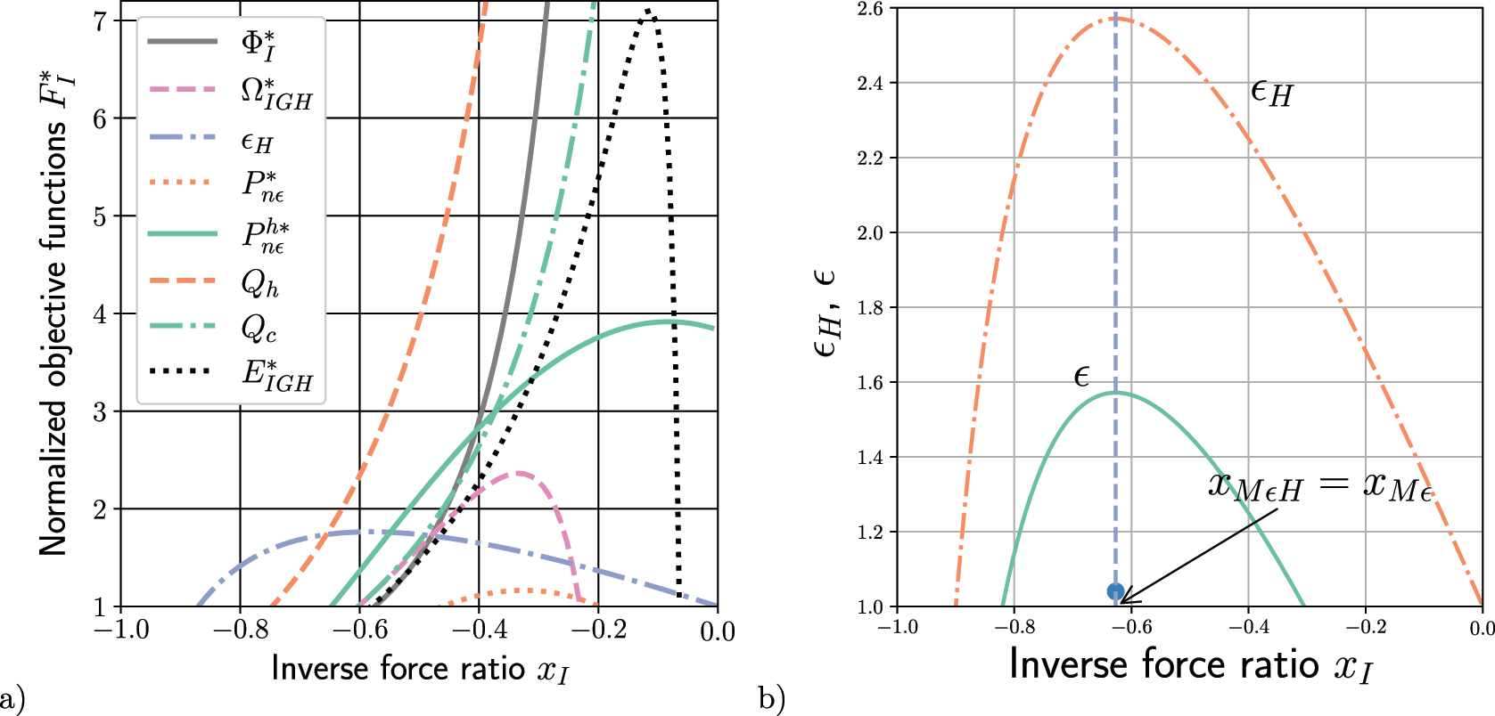
Energetics of the I-LEC. (a) In the figure, we can see the comparison of the different normalized objective functions, which are: heating dissipation function
This shows that ϵ H = 1 + ϵ is the classical relation between heating COP ϵ H and refrigeration COP ϵ. Now, by substituting Eq. (11b) and P = T h J I1 X 1 into ϵ H , we get:
In the same way we can calculate the maximum COP ϵ
MH
, for which we perform the optimization of Eq. (19) with respect to x
I
, and solving the equation
now, substituting Eq. (20) in Eq. (19) we obtain the maximum value of the heating COP ϵ MH ,
where, we have considered the Carnot’s COP ϵ
C
. Figure 2a shows the typical behavior of the COP and the heating COP, Eqs. (29 y 19), respectively, in comparison with other objective functions. Similarly, in Figure 2b, it can be observed that the classical relation ϵ
H
= 1 + ϵ holds. Additionally, the maximum values for the force ratio of the COP and the heating COP are evident, satisfying
On the other hand, we considered the definition of the generalized ecological function for both motor and refrigerator [1], [7], [8], with which it is possible that, we can propose the generalized heating ecological function E IGH , which we will define as follows,
where
substituting Eqs. (10), (18) and (23) in Eq. (22) is obtained,
Now we consider the generalized omega function for heat engines and refrigerators [1], [7], [11]. From the analysis and proper identification of effective useful energy E u,e and lost useful energy E l,u , we can propose the generalized heating Omega function Ω IGH . This objective function represents a balance between effective useful energy E u,e = E u − r min E i and lost useful energy E l,u = r max E i − E u . Here, E u is the machine’s useful energy, r min is the minimum performance, E i is the input energy, and r max is the maximum performance. Performance is defined as r = E u /E i . Finally, the generalized Omega function is defined as follows:
The function
or
in the equation Eq. (27) we have considered the first law, J h = P + J c and ϵ MH = 1 + ϵ M .
we can note that
3 Discussion on efficient power for I-LEC
In this section, we start from the already known concept of efficient power, P
η
, which is the product of power P and efficiency η, defined as P
η
= Pη [12]. This concept has been widely used in finite-time thermodynamics for thermal engines. Based on this, we propose three types of analogous functions for a system operated as an I-LEC (refrigerator and heat pump). The functions we developed are the efficient cooling power P
ϵ
, the efficient heating power P
Hϵ
, and the efficient combined cooling power
the optimal value of the force ratio, x Mϵ [1], is as follows:
We will define the generalized efficient cooling power as the product of the COP of refrigeration ϵ Eq. (29) (raised to the power n with
replacing Eq. (11b) and Eq. (15) in Eq. (31), we obtain,
This function shows a trade-off between the machine’s performance, the cooling COP, and the driven flux J
c
. This function presents an optimal value for the inverse force ratio x
I
, as can be observed in Figure 3a. Similarly, the optimal value is reported in Table 1. We will define the generalized combined efficient power
now replacing Eq. (11b) and Eq. (15) in

Generalized functions of efficient heating power-type functions. (a) The graph shows the plot of the generalized combined efficient power
The table shows the different optimal values obtained for each operating regime studied.
| I–LEC | Optimal value of the |
|---|---|
| Working regimes | Inverse force ratio
|
| ϵ H |
|
|
|
|
|
|
|
|
|
|
|
|
|
| Where: | |
|
|
This efficient power-type function demonstrates a trade-off between the machine’s performance, the cooling COP, and the driver flux J
h
. The function exhibits three optimal values for the inverse force ratio, as shown in Figure 3a. These optimal values are also listed in Table 1. The presence of multiple optimal points is further illustrated in Figure 3b, where the three roots
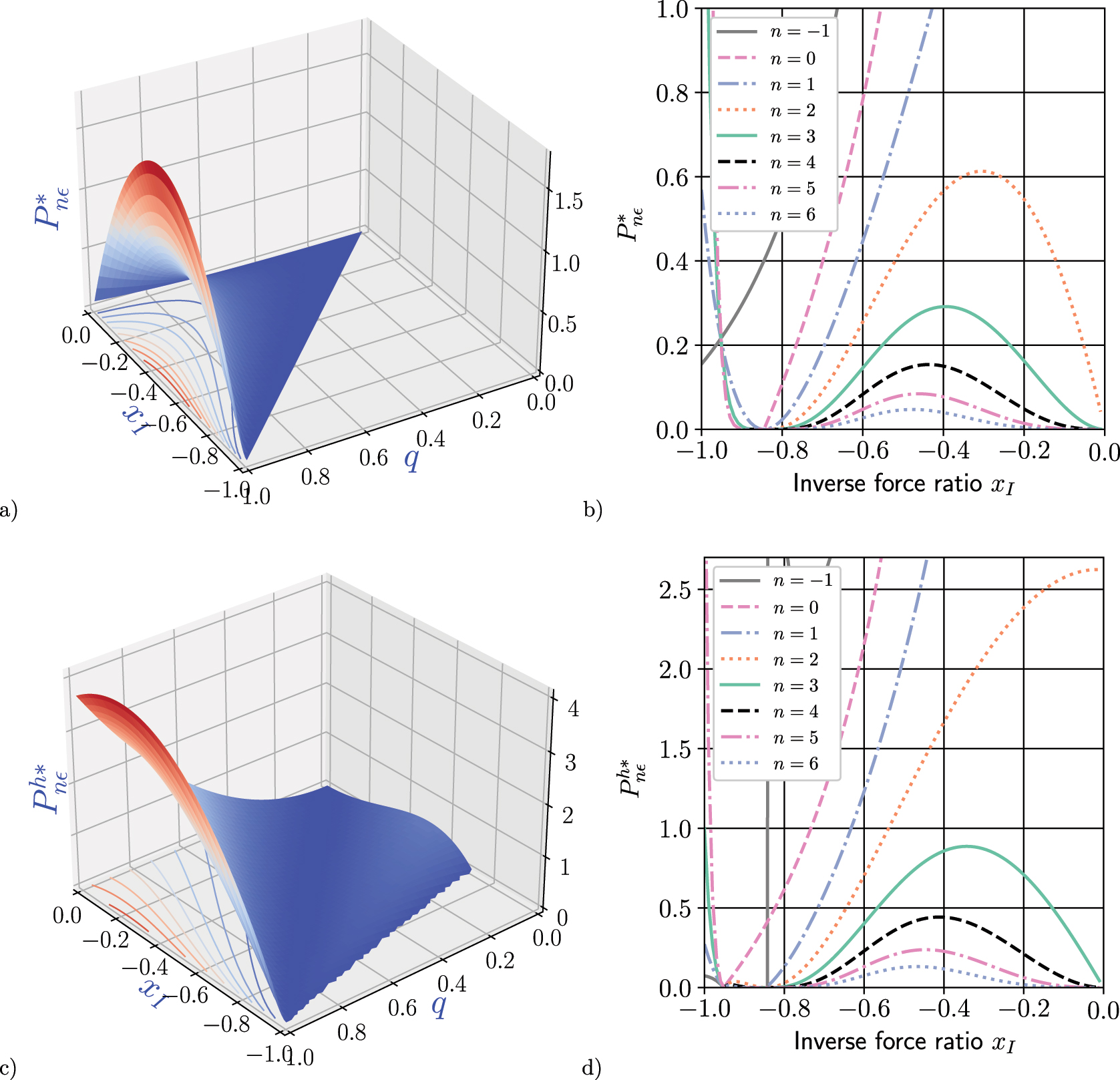
Generalized functions of efficient cooling power-type functions. (a) In the figure, we can see the generalized efficient cooling power
4 The thermoelectricity
As is well known, thermoelectricity encompasses a set of fundamental phenomena in Non-Equilibrium Thermodynamics. Among these, three principal effects stand out:
The Seebeck Effect: Discovered in 1821 by T. J. Seebeck, this effect involves the generation of electricity when heat is applied to the junction of two dissimilar materials.
The Peltier Effect: Observed in 1834 by Jean C. A. Peltier, this phenomenon manifests as a temperature gradient at the junction of two materials under isothermal conditions, caused by an electric current.
The Thomson Effect: Predicted and observed in 1851 by W. Thomson, this effect involves the heating or cooling of a current-carrying conductor in the presence of a temperature gradient.
L. Onsager, along with other researchers [2], [3], [13], [14], [15], [16], derived the phenomenological equations of the thermocouple. Starting from the entropy production of the thermoelectric phenomenon and incorporating the electrochemical potential, fluxes, and forces within the system, they obtained generalized equations describing these thermoelectric phenomena. These fundamental discoveries and theoretical developments have laid the groundwork for our modern understanding of thermoelectric processes, paving the way for numerous applications in energy conversion and thermal management systems.
4.1 Thermoelectric cooling and heating for an inverse linear energy converter (I-LEC)
Thermoelectric cooling and heating, as widely recognized, utilize the Peltier effect to create thermal flow across the junction of two different materials, typically P-type and N-type semiconductors. A Peltier device is a non-isothermal linear energy converter that transfers heat from one side to the other, against the temperature gradient, by consuming electrical energy. While heating can be achieved more economically through other methods, Peltier devices are valued for their compact size, lack of moving parts, and long durability. Importantly, they do not require liquids or refrigerant gases, making them environmentally friendly and suitable for various applications.
When connected to a direct current power source (such as a battery), as shown in Figure 1c, one side of the Peltier device cools while the other heats up. The efficiency of heat transfer depends on the supplied current and how effectively heat is removed from the hot side.
Additionally, Peltier devices can act as electrical generators if a temperature difference is maintained between the two sides, further increasing their versatility in energy conversion [1].
The phenomenological equations describing the behavior of these devices can be written as follows:
with J
1 = −J
N
and J
2 = J
Q
, the electrical current and the heat flux respectively,
where e is the electric charge. This approach establishes a direct relationship between measurable macroscopic properties (electrical and thermal conductivities) and the fundamental Onsager coefficients. By doing this, we bridge the gap between experimental observations and the theoretical framework of non-equilibrium thermodynamics. The thermal conductivity κ is defined as the heat flux per unit temperature gradient in the absence of an electric field in a homogeneous medium. Introducing this definition into Eq. (35), we obtain:
These direct coefficients corresponds to the well known phenomelogical laws, Ohm’s law and Fourier’s Law. The third phenomenological coefficient, which we will derive separately, is related to the thermoelectric power or Seebeck coefficient. Together, these three coefficients provide a complete description of the thermoelectric behavior of the system, enabling us to predict and optimize the performance of thermoelectric devices under various operating conditions. The derivation of the last coefficient is not trivial, but the deduction can be found in [1], yielding:
If we accept the electrical conductivity σ, thermal conductivity κ, and absolute thermoelectric power ɛ as the three physically significant dynamic properties of a medium, along with the force ratio and coupling constant, we can eliminate the three phenomenological coefficients and rewrite the kinetic equations (Eq. (35)) as follows:
The Peltier effect describes heat evolution at an isothermal junction (∇T = 0) due to an electric current. For this effect, we consider the electric potential X 1 = ∇μ/T as the driving force and the temperature gradient X 2 = −∇(1/T) as the driven force, measured between the welding points of materials A and B (see Figure 1a). We can construct the force ratio as follows:
This formulation provides a succinct description of the Peltier effect in terms of generalized thermodynamic forces, setting the stage for a more detailed analysis of thermoelectric phenomena. As we can observe from the force ratio x I determined in Eq. (40), we only need to provide the values of the electrical conductivity σ, the thermal conductivity κ, and the electric charge e to characterize the general behavior of the I − LEC, both when operated as a refrigerator or as a heat pump.
5 Concluding remarks
We considered a model in the context of LIT for a non-isothermal energy converter [1], with fixed temperatures (T and T + ΔT). This converter operates in two modes: as a direct linear energy converter (engine) or as an inverse linear energy converter (refrigerator or heat pump). In the latter, a spontaneous flux drives a non-spontaneous heat flux. Our study begins with the analysis of the second type, focusing on heat pumps. For this converter, we proposed and identified various steady-state operating regimes, which correspond to a specific relationship between the inverse force ratio x
I
and the coupling coefficient q. As noted in [1], x
I
relates to the machine’s operating mode, making it the target of most optimizations, while q concerns the converter’s design. In this framework, we proposed and analyzed several objective functions for inverse converters, specifically for heat pumps. We examined the following functions: the generalized heating ecological function
Generalized cooling functions. (a) In the figure, we can see the generalized efficient cooling power
6 Appendix
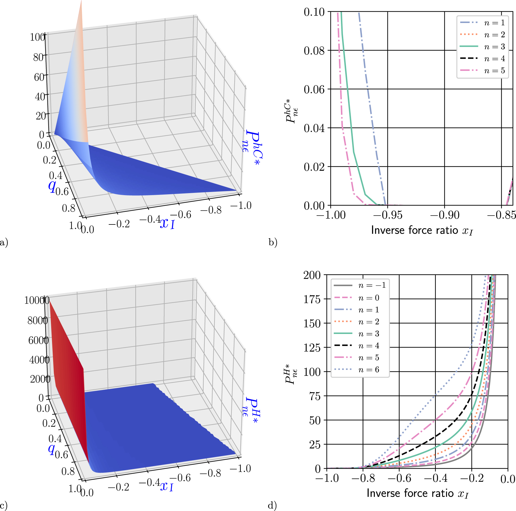
6.1 Generalized efficient heating power function’s
In this section, we propose and analyze a proposal for efficient power-type functions, as shown for refrigerators. To this end, we propose two possible generalized functions. Unfortunately, as we will see below, a proposal for this type of functions is not suitable for heat pumps, because, given the goal in energy conversion, the heating COP is not bounded, causing these types of functions to lack concavity and, therefore, an optimal value.
6.1.1 Generalized efficient heating power function’s
In analogy with the definition of generalized efficient power proposed in Section 3, we can propose two functions aimed at measuring the trade-off between the heating COP and one of the two flows involved in energy conversion. We will define the first type of generalized efficient heating power as the product of the heating COP, ϵ
H
Eq. (29) (raised to the power n with
obtaining,
On the other hand, we can propose that the conversion trade-off be between the flux J
h
and the heating COP, with which we will define the second type of generalized efficient heating power as the product of the heating COP, ϵ
H
Eq. (29) (raised to the power n with
obtaining,
The behavior of these two objective functions is shown in Figure 5. It can be observed that in the case of the type one function
Funding source: UNAM Postdoctoral Program (POSDOC)
-
Research ethics: Not applicable.
-
Informed consent: Not applicable.
-
Author contributions: The author has accepted responsibility for the entire content of this manuscript and approved its submission.
-
Use of Large Language Models, AI and Machine Learning Tools: To improve language.
-
Conflict of interest: The author states no conflict of interest.
-
Research funding: This work was supported by UNAM Postdoctoral Program (POSDOC).
-
Data availability: Not applicable.
References
[1] S. Gonzalez-Hernandez and L.-A. Arias-Hernandez, “Thermoelectric thomson relations revisited for a linear energy converter,” J. Non-Equilibrium Thermodyn., vol. 44, no. 3, pp. 315–332, 2019. https://doi.org/10.1515/jnet-2017-0068.Search in Google Scholar
[2] L. Onsager, “Reciprocal relations in irreversible processes. I,” Phys. Rev., vol. 37, no. 4, pp. 405–426, 1931. https://doi.org/10.1103/physrev.37.405.Search in Google Scholar
[3] L. Onsager, “Reciprocal relations in irreversible processes. II,” Phys. Rev., vol. 38, no. 12, pp. 2265–2279, 1931. https://doi.org/10.1103/physrev.38.2265.Search in Google Scholar
[4] J. W. Stucki, “The optimal efficiency and the economic degrees of coupling of oxidative phosphorylation,” Eur. J. Biochem., vol. 109, no. 1, pp. 269–283, 1980. https://doi.org/10.1111/j.1432-1033.1980.tb04792.x.Search in Google Scholar PubMed
[5] L. A. Arias-Hernandez, F. Angulo-Brown, and R. T. Paez-Hernandez, “First-order irreversible thermodynamic approach to a simple energy converter,” Phys. Rev. E, vol. 77, no. 1, p. 011123, 2008. https://doi.org/10.1103/physreve.77.011123.Search in Google Scholar PubMed
[6] S. R. Caplan and A. Essig, Bioenergetics and Linear Nonequilibrium Thermodynamics: The Steady State, 1st ed., Cambridge, MA, Ed. Harvad University Press, 1983.10.4159/harvard.9780674732063Search in Google Scholar
[7] L. Partido Tornez, Aplicación del criterio omega y ecológico generalizados a diferentes convertidores de energía, Tesis de Maestría, México, ESFM-IPN, 2006.Search in Google Scholar
[8] F. Angulo Brown, “An ecological optimization criterion for finite-time heat engines,” J. Appl. Phys., vol. 69, no. 11, pp. 7465–7469, 1991.10.1063/1.347562Search in Google Scholar
[9] F. Angulo–Brown and L. A. Arias–Hernandez, “Reply to Comment on: A general property of endoreversible thermal engines,” J. Appl. Phys., vol. 89, pp. 1520–1521, 2001, https://doi.org/10.1063/1.1335619.Search in Google Scholar
[10] L. A. Arias-Hernandez, G. Ares de Parga, and F. Angulo-Brown, “On some nonendoreversible engine models with nonlinear heat transfer laws,” Open Syst. Inf. Dynam., vol. 10, no. 4, pp. 351–375, 2003.10.1023/B:OPSY.0000009556.27759.11Search in Google Scholar
[11] A. Calvo-Hernández, A. Medina, J. M. M. Roco, J. A. White, and S. Velasco, “Unified optimization criterion for energy converters,” Phys. Rev. E, vol. 63, pp. 37102–37111, 2001, https://doi.org/10.1103/physreve.63.037102.Search in Google Scholar PubMed
[12] T. Yilmaz, “A new performance criterion for heat engines: Efficient power,” J. Energy Inst., vol. 79, no. 1, pp. 38–41, 2006. https://doi.org/10.1179/174602206x90931.Search in Google Scholar
[13] H. B. Callen, Thermodynamics and an Introduction to Thermostatistics, Canada, Wiley, 1985.Search in Google Scholar
[14] H. B. Callen, “The application of Onsager’s reciprocal relations to thermoelectric, thermomagnetic, and galvanomagnetic effects,” Phys. Rev., vol. 73, no. 11, pp. 1349–1358, 1948. https://doi.org/10.1103/physrev.73.1349.Search in Google Scholar
[15] S. R. De Groot and P. Mazur, Non-Equilibrium Thermodynamics, New York, Dover Publications, 1984.Search in Google Scholar
[16] L. García Colín-Scherer and P. Goldstein Menache, La física de los procesos irreversibles, México, El Colegio Nacional, 2003.Search in Google Scholar
© 2025 the author(s), published by De Gruyter, Berlin/Boston
This work is licensed under the Creative Commons Attribution 4.0 International License.
Articles in the same Issue
- Frontmatter
- Original Research Articles
- Modeling high-pressure viscosities of fatty acid esters and biodiesel fuels based on modified rough hard-sphere-chain model and deep learning method
- Study on heat and mass transfer mechanism of unsaturated porous media under CW laser irradiation: with and without carrier gas
- Efficient ecological function optimization for endoreversible Carnot heat pumps
- Entropy as Noether charge for quasistatic gradient flow
- Numerical simulation of binary convection within the Soret regime in a tilted cylinder
- Is there a need for an extended phase definition for systems far from equilibrium?
- Existence of the Chapman–Enskog solution and its relation with first-order dissipative fluid theories
- Performance comparison of water towers and combined pumped hydro and compressed gas system and proposing a novel hybrid system to energy storage with a case study of a 50 MW wind farm
- Thermodynamic characterization of transient valve temperatures in diesel engines using probabilistic methods
- Energetic analysis of a non-isothermal linear energy converter operated in reverse mode (I-LEC): heat pump