Home On the singular loci of higher secant varieties of Veronese embeddings
Article Open Access

On the singular loci of higher secant varieties of Veronese embeddings

  • Katsuhisa Furukawa and Kangjin Han ORCID logo EMAIL logo
Published/Copyright: April 30, 2025

Abstract

The 𝑘-th secant variety of a projective variety X P N , denoted by σ k ( X ) , is defined to be the closure of the union of ( k 1 ) -planes spanned by 𝑘 points on 𝑋. In this paper, we examine the 𝑘-th secant variety σ k ( v d ( P n ) ) P N of the image of the 𝑑-uple Veronese embedding v d of P n to P N with N = ( n + d d ) 1 , and focus on the singular locus of σ k ( v d ( P n ) ) , which is only known for k 3 . To study the singularity for arbitrary k , d , n , we define the 𝑚-subsecant locus of σ k ( v d ( P n ) ) to be the union of σ k ( v d ( P m ) ) with any 𝑚-plane P m P n . By investigating the projective geometry of moving embedded tangent spaces along subvarieties and using known results on the secant defectivity and the identifiability of symmetric tensors, we determine whether the 𝑚-subsecant locus is contained in the singular locus of σ k ( v d ( P n ) ) or not. Depending on the value of 𝑘, these subsecant loci show an interesting trichotomy between generic smoothness, non-trivial singularity, and trivial singularity. In many cases, they can be used as a new source for the singularity of the 𝑘-th secant variety of v d ( P n ) other than the trivial one, the ( k 1 ) -th secant variety of v d ( P n ) . We also consider the case of the fourth secant variety of v d ( P n ) by applying main results and computing conormal space via a certain type of Young flattening. Finally, we present some generalizations and discussions for further developments.

1 Introduction

Throughout the paper, we work over ℂ, the field of complex numbers. Let X P N be an embedded projective variety. The 𝑘-th secant variety of 𝑋 is defined as

(1.1) σ k ( X ) = x 1 , , x k X x 1 , , x k ̄ P N ,

where x 1 , , x k P N denotes the linear span of the points x 1 , , x k and the overline means the Zariski closure. In particular, σ 1 ( X ) = X and σ 2 ( X ) is often simply called the secant or secant line variety of 𝑋 in the literature.

The construction of secant varieties (or more generally, join construction of subvarieties) is not only one of the most famous methods in classical algebraic geometry, but also a very popular subject in recent years, especially in connection with fields of research such as tensor rank and decomposition, algebraic statistics, data science, geometric complexity theory, and so on (see [22, 23] for more details).

Despite of a rather long history and the popularity, most of the fundamental questions on the higher secant varieties σ k ( X ) still remain open even for many well-known base varieties 𝑋. For instance, one can ask the secant defectivity question, which concerns the dimension of σ k ( X ) . We say that σ k ( X ) is secant defective (or simply defective) if the dimension of σ k ( X ) is less than the expected one, min { N , k dim ( X ) + k 1 } . It is classically known that higher secant varieties of curves are non-defective (e.g. [29, Corollary 1.2.3]). Due to the famous theorem of Alexander–Hirschowitz [2], we know the dimensions of higher secant varieties of all Veronese varieties. In other research, there are only a few cases where the dimension theorem for σ k ( X ) is fully determined (see [29, 30] for references). Questions about defining equations of 𝑘-th secant varieties have also only been answered for very small 𝑘 of a few cases and seem still far from understanding the essence of the sources for the equations (see also [22, Chapter 5] for a reference).

In this paper, we concentrate on the case of X = v d ( P n ) P N , the Veronese variety, which is the image of the Veronese embedding v d : P n P N with N = ( n + d d ) 1 . In particular, we study the singular locus of σ k ( v d ( P n ) ) , an arbitrary higher secant variety of the Veronese variety.

The knowledge on singularities of higher secant varieties is fundamental and very important for its own sake in the study of algebraic geometry and also can be useful for problems in applications. For example, it can be used as a key condition to establish the identifiability of structured tensors (e.g. the introduction in [7] and references therein).

For any irreducible variety X P N , it is classically well known that

(1.2) σ k 1 ( X ) Sing ( σ k ( X ) )

unless σ k ( X ) fills up the whole linear span X (see [29, Proposition 1.2.2]). In the paper, we say that a point p σ k ( X ) is a non-trivial singular point if p σ k 1 ( X ) and σ k ( X ) is singular at 𝑝, while the points belonging to σ k 1 ( X ) are called trivial singular points.

There are some known results on the singular loci of 𝑘-th secant varieties σ k ( X ) , mostly for very small 𝑘. The equality in (1.2) holds for determinantal varieties defined by minors of a generic matrix. It is completely described for the second secant variety of the Segre product of projective spaces in [28]. It has recently been generalized to the case of σ 2 ( X ) , where 𝑋 is a Segre–Veronese embedding by [21] and 𝑋 is a Grassmannian by [13]. For the third secant variety of the Grassmannian G ( 2 , 6 ) , the dimension and some other properties of the singularity have been studied in [1].

For the case of Veronese varieties, it is classical that Sing ( σ k ( v d ( P n ) ) ) = σ k 1 ( v d ( P n ) ) holds both for the binary case (i.e., n = 1 ) and for the case of quadratic forms (i.e., d = 2 ) (see e.g. [19, Chapter 1]). For k = 2 , it was proved in [20] that the above equality holds also for any d , n . In these cases, the 𝑘-th secant variety has only the trivial singularity. For k = 3 , the singular locus was completely determined by the second author in [16]; in particular, the non-trivial singularity occurs if and only if d = 4 and n 3 .

In the present paper, we explore the singular locus of any higher secant variety of the Veronese variety, and introduce a new main origin for the singularity other than the trivial singularity. We call this the “subsecant locus”. As in our main results, these loci show an interesting trichotomy phenomenon among generic smoothness, non-trivial singularity, and trivial singularity.

For any given point p σ k ( v d ( P n ) ) , there exists an 𝑚-plane (i.e., 𝑚-dimensional linear subvariety) P m of P n with 1 m k 1 such that p σ k ( v d ( P m ) ) ; it immediately follows for a general 𝑝, and even if 𝑝 is in the boundary of the closure in (1.1), it is also true by considering ( 1 , d 1 ) -symmetric flattening (see Section 3 for details). So, from now on, we say that σ k ( v d ( P m ) ) σ k ( v d ( P n ) ) is an 𝑚-subsecant variety of σ k ( v d ( P n ) ) if m < k 1 and m < n , and simply call it a subsecant variety in case there is no confusion. We also define the 𝑚-subsecant locus of σ k ( v d ( P n ) ) ,

(1.3) Σ k , d ( m ) or Σ k , d ( m ; P n ) = P m P n σ k ( v d ( P m ) ) .

It naturally forms an increasing sequence of loci in the 𝑘-th secant variety as

Σ k , d ( 1 ) Σ k , d ( 2 ) Σ k , d ( min { k 1 , n } 1 ) σ k ( v d ( P n ) ) = Σ k , d ( min { k 1 , n } ) .

In particular, we have that Σ k , d ( min { k 1 , n } 1 ) is the union of all proper subsecant varieties, which we call the maximum subsecant locus of the given 𝑘-th secant variety σ k ( v d ( P n ) ) . Any point of σ k ( v d ( P n ) ) outside the maximum subsecant locus and the previous secant variety σ k 1 ( v d ( P n ) ) is called a point of the full-secant locus. Note that, for k = 3 of [16], when d = 4 and n 3 , the singular locus of σ 3 ( v d ( P n ) ) is given as the maximum subsecant locus Σ 3 , d ( 1 ) , which is the only case where the singularity pattern of the third secant varieties becomes exceptional, while for all the other d , n , the singularity is just the trivial one, σ 2 ( v d ( P n ) ) (see Remark 4 (a)). Most of the previously known results on singular loci of secant varieties can be understood in this viewpoint (see Remark 37).

Thus a basic question for our concern could be stated as follows: for given k , d , m , n ,

when is σ k ( v d ( P n ) ) singular at points of an m -subsecant locus Σ k , d ( m ) ?

In principle, it is somewhat straightforward (despite the computational complexity) to check the singularity, once a complete set of equations for a higher secant variety is attained. But, as mentioned above, not much is known about the defining equations and they seem quite far from being fully understood at this moment, even for the Veronese case (see [24, 11] for the state of the art). Due to the lack of knowledge on the equations for the higher secant variety, it is very difficult to determine the singular locus in general.

In this paper, without further understanding on the equations (!), we introduce a geometric way to pursue it for this kind of problems, which is based on a careful study on the behavior of embedded tangent spaces moving along a locus in the Veronese variety. For the case m = 1 , we first present the following result for the 1-subsecant locus Σ k , d ( 1 ) = P 1 P n σ k ( v d ( P 1 ) ) of σ k ( v d ( P n ) ) , which is a generalization of [16, Theorem 2.1] (i.e., k = 3 case) to any higher 𝑘-th secant varieties of Veronese varieties.

Theorem 1

Let v d : P n P N be the 𝑑-uple Veronese embedding with n 2 , d 3 , and N = ( n + d d ) 1 . Assume k 3 . For ( k , d , n ) ( 3 , 4 , 2 ) , the following holds.

  1. If k d + 1 2 , then σ k ( v d ( P n ) ) is smooth at every point in Σ k , d ( 1 ) σ k 1 ( v d ( P n ) ) .

  2. If k = d + 2 2 , then Σ k , d ( 1 ) Sing ( σ k ( v d ( P n ) ) ) but Σ k , d ( 1 ) σ k 1 ( v d ( P n ) ) (i.e., non-trivial singularity). This case occurs only if 𝑑 is even.

  3. If k d + 3 2 , then Σ k , d ( 1 ) σ k 1 ( v d ( P n ) ) (i.e., trivial singularity, unless we have that σ k ( v d ( P n ) ) = P N ).

For ( k , d , n ) = ( 3 , 4 , 2 ) , it holds that
  1. σ 3 ( v 4 ( P 2 ) ) is smooth at every point in Σ 3 , 4 ( 1 ) σ 2 ( v 4 ( P 2 ) ) .

Concerning singular points of arbitrary σ k ( v d ( P n ) ) originated from subsecant loci, we prove the following general theorems on the 𝑚-subsecant locus Σ k , d ( m ) with m 2 and k 4 as the main results.

Theorem 2

Let v d : P n P N be the 𝑑-uple Veronese embedding with n 3 , d 3 , and N = ( n + d d ) 1 . Let k 4 and let P m P n be an 𝑚-plane with 2 m < min { k 1 , n } . Assume that ( d , m ) E = { ( 3 , 3 ) , ( 3 , 4 ) , ( 3 , 5 ) , ( 4 , 2 ) , ( 4 , 3 ) , ( 4 , 4 ) , ( 5 , 2 ) , ( 6 , 2 ) } .

For ( k , d , n ) ( 4 , 3 , 3 ) , setting

μ = ( m + d m ) m + 1 ,

we have the following.

  1. If k < μ , then σ k ( v d ( P n ) ) is smooth at a general point in Σ k , d ( m ) σ k 1 ( v d ( P n ) ) .

  2. If k = μ , then Σ k , d ( m ) Sing ( σ k ( v d ( P n ) ) ) but Σ k , d ( m ) σ k 1 ( v d ( P n ) ) (i.e., non-trivial singularity).

  3. If k > μ , then Σ k , d ( m ) σ k 1 ( v d ( P n ) ) (i.e., trivial singularity, unless we have that σ k ( v d ( P n ) ) = P N ).

For ( k , d , n ) = ( 4 , 3 , 3 ) , it holds that
  1. σ 4 ( v 3 ( P 3 ) ) is smooth at every point in Σ 4 , 3 ( 2 ) σ 3 ( v 3 ( P 3 ) ) .

Theorem 3

In the same situation as Theorem 2, for

( d , m ) E = { ( 3 , 3 ) , ( 3 , 4 ) , ( 3 , 5 ) , ( 4 , 2 ) , ( 4 , 3 ) , ( 4 , 4 ) , ( 5 , 2 ) , ( 6 , 2 ) } ,

if 𝑘 is in one of the ranges named (i), (ii), (iii) in Table 1, then the following property corresponding to the name of the range holds.

  1. σ k ( v d ( P n ) ) is smooth at a general point in Σ k , d ( m ) σ k 1 ( v d ( P n ) ) .

  2. Σ k , d ( m ) Sing ( σ k ( v d ( P n ) ) ) but Σ k , d ( m ) σ k 1 ( v d ( P n ) ) .

  3. Σ k , d ( m ) σ k 1 ( v d ( P n ) ) .

Table 1

(Non-)singularity of Σ k , d ( m ) in Theorem 3

( d , m ) ( m + d m ) m + 1 (i) (ii) (iii)
( 3 , 3 ) 5 k 5 None 6 k
( 3 , 4 ) 7 k 6 k = 7 , 8 9 k
( 3 , 5 ) 28/3 k 8 k = 9 , 10 11 k
( 4 , 2 ) 5 k 4 k = 5 , 6 7 k
( 4 , 3 ) 35/4 k 7 k = 8 , 9 , 10 11 k
( 4 , 4 ) 14 k 13 k = 14 , 15 16 k
( 5 , 2 ) 7 k 7 None 8 k
( 6 , 2 ) 28/3 k 8 k = 9 , 10 11 k

To understand the reason for considering the conditions that ( d , m ) is in ℰ or not, we discuss the secant defectivity and the generic identifiability of an 𝑚-subsecant variety

σ k ( v d ( P m ) ) σ k ( v d ( P n ) ) .

Set P β = v d ( P m ) P N with β = ( m + d m ) 1 , where σ k ( v d ( P m ) ) P β is of dimension at most k m + k 1 .

By [2], the codimension of σ k ( v d ( P m ) ) in P β is greater than max { β ( k m + k 1 ) , 0 } (i.e., σ k ( v d ( P m ) ) does not fill P β and is secant defective) if and only if d = 2 and 2 k m , or ( k , d , m ) = ( 7 , 3 , 4 ) , ( 5 , 4 , 2 ) , ( 9 , 4 , 3 ) , ( 14 , 4 , 4 ) ; indeed, in the latter case, the four 𝑘-th secant varieties σ k ( v d ( P m ) ) are hypersurfaces of P β . Except these defective cases, we have σ k ( v d ( P m ) ) = P β if k m + k 1 β , or equivalently k ( m + d m ) / ( m + 1 ) .

We say a point a P β is 𝑘-identifiable if there is a unique𝑘-tuple of points x 1 , , x k in v d ( P m ) such that a x 1 , , x k . We also say that σ k ( v d ( P m ) ) is generically identifiable if a general point a σ k ( v d ( P m ) ) is 𝑘-identifiable. From [14, Theorem 1], a general point a P β is 𝑘-identifiable (or σ k ( v d ( P m ) ) is generically identifiable in the case of σ k ( v d ( P m ) ) = P β ) if and only if m = 1 and k = ( d + 1 ) / 2 , or ( k , d , m ) = ( 5 , 3 , 3 ) , ( 7 , 5 , 2 ) . From [8, Theorem 1.1], when σ k ( v d ( P m ) ) P β is not secant defective, σ k ( v d ( P m ) ) is not generically identifiable if and only if ( k , d , m ) = ( 9 , 3 , 5 ) , ( 8 , 4 , 3 ) , ( 9 , 6 , 2 ) .

Remark 4

We make some remarks on the theorems above.

(a) In the case of k = 3 and n 3 , Theorem 1 (ii) holds if and only if d = 4 , and then Sing ( σ 3 ( v 4 ( P n ) ) is equal to P 1 P n v 4 ( P 1 ) = Σ 3 , 4 ( 1 ) since σ 3 ( v 4 ( P 1 ) ) = v 4 ( P 1 ) and σ 2 ( v 4 ( P n ) ) P 1 P n v 4 ( P 1 ) (see also Corollary 32). This gives a geometric description of the only exceptional case for the singular loci of the third secant varieties in [16].

(b) Theorem 1 (i) is stronger than Theorems 2 (i) and 3 (i), since it claims smoothness for “every point” in the 𝑚-subsecant locus Σ k , d ( m ) outside σ k 1 ( v d ( P n ) ) . The “general point” condition in Theorems 2 (i) and 3 (i) cannot be deleted (see Example 27). We also note that the ranges of 𝑘 of (i) and (ii) are slightly different between Theorems 1 and 2. If m = 1 and 𝑑 is even, then the case k = ( m + d m ) / ( m + 1 ) = ( d + 2 ) / 2 is Theorem 1 (ii), which is similar to Theorem 2 (ii); for this 𝑘, σ k ( v d ( P 1 ) ) is not generically identifiable. However, if 𝑑 is odd, then the case k = ( m + d m ) / ( m + 1 ) = ( d + 1 ) / 2 belongs to Theorem 1 (i).

(c) Theorems 1 (i), 2 (i), and 3 (i) correspond to the 𝑘-identifiable case of a general point a σ k ( v d ( P m ) ) . From the viewpoint of the secant fiber in incidence (2.1), this means that the fiber p 1 ( a ) under the projection 𝑝 consists of only one element up to permuting x i . On the other hand, Theorems 1 (ii), 2 (ii), and 3 (ii) correspond to the case of generic non-identifiability of the subsecant variety σ k ( v d ( P m ) ) with the situation of σ k 1 ( v d ( P m ) ) P β = v d ( P m ) , except ( k , d , m , n ) = ( 3 , 4 , 1 , 2 ) , ( 4 , 3 , 2 , 3 ) . This non-identifiability of a general point 𝑎 in σ k ( v d ( P m ) ) occurs if dim p 1 ( a ) > 0 , or if dim p 1 ( a ) = 0 and # p 1 ( a ) 2 (modulo permutation). For m = 1 , only the former occurs when k = ( d + 2 ) / 2 . For m 2 , the former corresponds to the case where 𝑘 is the ceiling of ( m + d m ) / ( m + 1 ) N with σ k ( v d ( P m ) ) = P β , to the case where σ k ( v d ( P m ) ) P β is defective, or to the case where σ k 1 ( v d ( P m ) ) P β is defective (i.e., ( k , d , m ) = ( 8 , 3 , 4 ) , ( 6 , 4 , 2 ) , ( 10 , 4 , 3 ) , ( 15 , 4 , 4 ) ), and the latter corresponds to the case where 𝑘 is the number ( m + d m ) / ( m + 1 ) N with σ k ( v d ( P m ) ) = P β except for ( k , d , m ) = ( 5 , 3 , 3 ) , ( 7 , 5 , 2 ) , or to the case ( k , d , m ) = ( 9 , 3 , 5 ) , ( 8 , 4 , 3 ) , ( 9 , 6 , 2 ) .

(d) ( k , d , m , n ) = ( 3 , 4 , 1 , 2 ) , ( 4 , 3 , 2 , 3 ) (i.e., Theorems 1 (iv) and 2 (iv)), a posteriori, turn out to be the only two exceptional cases which do not follow this trichotomy pattern; in other words, though 𝑘 belongs to the range of (ii) and the generic non-identifiability of σ k ( v d ( P m ) ) holds, Σ k , d ( m ) does not provide non-trivial singular points (see also Remark 24). Indeed, in [11], we show that if ( k , d , n ) = ( 3 , 4 , 2 ) , ( 4 , 3 , 3 ) , then σ k ( v d ( P n ) ) is a del Pezzo 𝑘-th secant variety, that is, a 𝑘-th secant variety of next-to-minimal degree. In this sense, these two cases also belong to a special class with respect to the degrees of higher secant varieties. (For basic definitions and results on such varieties, see [10, 9].)

As an application of our main results for Σ 4 , d ( 2 ) and Σ 4 , d ( 1 ) , we obtain the following result on the singularity of the fourth secant variety of any Veronese variety.

Theorem 5

Theorem 5 (Singular locus for σ 4 ( v d ( P n ) ) )

Let v d : P n P N be the 𝑑-uple Veronese embedding with n 3 , d 3 , and N = ( n + d d ) 1 . Then the following holds.

  1. σ 4 ( v d ( P n ) ) is smooth at every point outside Σ 4 , d ( 2 ) σ 3 ( v d ( P n ) ) .

  2. If d 4 , a general point in Σ 4 , d ( 2 ) σ 3 ( v d ( P n ) ) is also a smooth point of σ 4 ( v d ( P n ) ) . When d = 3 and n = 3 , all points in Σ 4 , d ( 2 ) σ 3 ( v d ( P n ) ) are smooth. If d = 3 and n 4 , then Σ 4 , d ( 2 ) Sing ( σ 4 ( v d ( P n ) ) ) but Σ 4 , d ( 2 ) σ 3 ( v d ( P n ) ) (i.e., non-trivial singularity).

  3. For d 7 , all points in Σ 4 , d ( 1 ) σ 3 ( v d ( P n ) ) σ 4 ( v d ( P n ) ) are smooth. When d = 6 , Σ 4 , d ( 1 ) Sing ( σ 4 ( v d ( P n ) ) ) but Σ 4 , d ( 1 ) σ 3 ( v d ( P n ) ) (i.e., non-trivial singularity). When d 5 , Σ 4 , d ( 1 ) σ 3 ( v d ( P n ) ) (i.e., trivial singularity).

For a projective variety X P N , we denote by Vertex ( X ) the set of vertices of 𝑋. Then 𝑋 is a cone if and only if Vertex ( X ) .

Example 6

Example 6 (Cases with a nice description)

The smallest case for the singular locus of σ 4 ( v d ( P n ) ) beyond the classical results for d = 2 or n = 1 is ( d , n ) = ( 3 , 2 ) , but in this case, there is nothing to check because σ 4 ( v 3 ( P 2 ) ) fills up the ambient space P 9 and then Sing ( σ 4 ( v 3 ( P 2 ) ) ) = . In the case ( d , n ) = ( 3 , 3 ) , by Theorem 5 (i) and (ii), we have

Sing ( σ 4 ( v 3 ( P 3 ) ) ) = σ 3 ( v 3 ( P 3 ) ) .

For the case ( d , n ) = ( 3 , 4 ) , if 𝑉 denotes a 5-dimensional ℂ-vector space with P 4 = P V , Theorem 5 tells us that the singular locus of the fourth secant variety of v 3 ( P V ) in P 34 is precisely the locus of cubic hypersurfaces in five variables which are cones with the vertex dimension at least 1 as follows:

Sing ( σ 4 ( v 3 ( P V ) ) ) = σ 3 ( v 3 ( P V ) ) Σ 4 , 3 ( 2 ; P V )
= σ 3 ( v 3 ( P V ) ) { P 2 P V σ 4 ( v 3 ( P 2 ) ) } = P 2 P V v 3 ( P 2 )
= { f P S 3 V the cubic hypersurface X P V defined by f
is a cone with dim Vertex ( X ) 1 } ,
which is just the maximum subsecant locus Σ 4 , 3 ( 2 ; P V ) , an irreducible 15-dimensional locus in the 19-dimensional variety σ 4 ( v 3 ( P V ) ) . By the same argument, we can obtain

Sing ( σ 4 ( v 3 ( P n ) ) ) = Σ 4 , 3 ( 2 ; P n ) for any n 4 .

Such a simple description of the singular locus can be attained in a few more cases (see Corollary 32 for details).

The paper is structured as follows. In Section 2, as preparation, we first recall some preliminaries on 𝑘-th secant varieties and corresponding incidences. Then, using projective techniques, such as Terracini’s lemma, the trisecant lemma, descriptions of embedding tangent spaces, and tangential projections, we reveal several geometric properties of 𝑚-subsecant varieties in higher secant varieties of Veronese varieties, which are crucial for the proof of the main theorems. In Section 3, as an illustration of the whole picture and our main ideas, we treat the case m = 1 and prove Theorem 1. In Section 4, we deal with the general case (i.e., m 2 ) and prove Theorem 2 and Theorem 3 to generalize the ideas used in the previous section. We would like to remark that this can be done because the dimension theorem [2] and the generic identifiability question [8, 14] were settled for the case of Veronese varieties. In Section 5, we focus on the singular locus of the fourth secant variety and prove Theorem 5 by dividing the case into two parts: “full-secant locus points (i.e., m = 3 )” treated in Theorem 29 via Young flattening and conormal space computation and “the subsecant locus” by Corollary 30. Finally, we make some generalizations and remarks on the material for further developments in Section 6.

2 Some geometric properties of subsecant varieties

2.1 Projection from the incidence to the secant variety

For a (reduced and irreducible) variety 𝑋, we denote X × × X , the (usual) product of 𝑘 copies of 𝑋, by ( X ) k . We denote the 𝑘-fold symmetric product of 𝑋, ( X ) k / S n , by Sym k ( X ) .

For the 𝑑-uple Veronese embedding v d : P n P N with N = ( n + d d ) 1 , we regard the incidence variety I = I ( n ) P N × ( P n ) k to be the Zariski closure of

(2.1) I 0 = I ( n ) 0 = { ( a , x 1 , , x k ) a x 1 , , x k and dim x 1 , , x k = k 1 } ,

where we write x i = v d ( x i ) for x i P n . Taking the first projection p : I P N , we have p ( I ) = σ k ( v d ( P n ) ) (see also [29, Definition 1.1.3], [30, Chapter I, §1, Chapter V]). For any a σ k ( v d ( P n ) ) , p 1 ( a ) is often called the secant fiber of 𝑎. Note that 𝐼 is invariant under permuting factors on ( P n ) k from the definition so that both 𝑝 and q i maps factor through P N × Sym k ( P n ) .

We also have dim I = n k + k 1 by considering general fibers of q : I ( P n ) k . For each 1 i k , let q i : I ( P n ) k P n be the composition of 𝑞 and the projection to the 𝑖-th factor ( P n ) k P n . Then the following commutative diagram is obtained:

Remark 7

We have some remarks on the incidence variety I P N × ( P n ) k .

(a) I 0 can be viewed as a P k 1 -bundle over a non-empty open subset 𝑈 of ( P n ) k , consisting of 𝑘-tuples of points with the expected spanning dimension, so that 𝐼 is irreducible. Further, for q 1 ( U ) = I ( P n × U ) , we have I 0 = q 1 ( U ) since both are irreducible closed subsets in P N × U having the same dimension. So, for any ( a , x 1 , , x k ) I I 0 and for x i = v d ( x i ) , dim x 1 , , x k < k 1 (in other words, there is no ( a , x 1 , , x k ) I I 0 such that dim x 1 , , x k = k 1 but a x 1 , , x k ). Finally, note that the Euclidean closure of I 0 also coincides with 𝐼 in this case (see e.g. [23, Theorem 3.1.6.1]).

(b) In the case of dim σ k ( v d ( P n ) ) = n k + k 1 , it holds p ( I I 0 ) σ k ( v d ( P n ) ) , and then p 1 ( a ) I 0 for general a σ k ( v d ( P n ) ) . In addition, if k ( n + d 1 n ) , then setting

D = { ( x 1 , , x k ) ( P n ) k dim ( v d 1 ( x 1 ) , , v d 1 ( x k ) ) < k 1 } ,

we have dim ( I ( P N × D ) ) < dim ( I ) , and hence p ( I ( P N × D ) ) σ k ( v d ( P n ) ) .

(c) (Alternative incidences for the 𝑘-th secant variety) In the literature, instead of ( X ) k , other spaces such as the symmetric product Sym k ( X ) (e.g. in [8]), the Hilbert scheme of degree 𝑘 0-dimensional subschemes Hilb k ( X ) (e.g. in [5]), and the Grassmannian G ( k 1 , N ) (e.g. in [27]) have also been used in the incidence to consider the 𝑘-th secant variety of X P N .

Remark 8

Let us fix an 𝑚-plane L = P m P n and consider the 𝑑-uple Veronese embedding of P m , v d : L = P m P β with β = ( m + d m ) 1 . We often use the following notation.

(a) Let L ̂ P n be any ( n m 1 ) -plane not intersecting 𝐿. Changing homogeneous coordinates t 0 , t 1 , , t m , u 1 , u 2 , , u m on P n with m = n m , we may assume that L P n is the zero set of u 1 , , u m and L ̂ P n is the zero set of t 0 , , t m . For any x i P n , say

x i = [ x i , 0 : : x i , m : x i , m + 1 : : x i , n ] P n ,

then we set y i = [ x i , 0 : : x i , m : 0 : : 0 ] . Thus y i gives a point of the 𝑚-plane if x i is not of the form [ 0 : : 0 : : : ] . By abuse of notation, we denote by y i both corresponding points in P m and in P n . Further, considering linear projections π 1 : P n P m from the center L ̂ (eliminating the 𝑢-variables), and π 2 : P N P β (eliminating all the monomials of degree 𝑑 which involve 𝑢-variables), we have a natural commuting diagram as v d π 1 = π 2 v d ,

(2.2)

In particular, when d = 2 and n = m + 1 (i.e., m = 1 ), then π 1 is an (inner) projection from one point a P n and π 2 corresponds to a tangential projection of P N from T v 2 ( a ) v 2 ( P n ) .

(b) On the affine open subset { t 0 0 } , the 𝑑-uple Veronese embedding v d : P n P N is parameterized by monomials in mono [ t , u ] d , where mono [ t , u ] e (resp. mono [ t ] e ) is defined to be the set of monomials in C [ t 1 , , t m , u 1 , , u m ] (resp. in C [ t 1 , , t m ] ) of degree at most 𝑒 for an integer 𝑒.

Let us study the behavior of some points in the boundary of 𝐼, which belong to 𝐼 but do not belong to I 0 , as follows.

Lemma 9

Let L = P m P n be any 𝑚-plane with m < n , and consider

P β = v d ( L ) P N .

For v d : L = P m P β , let us take I ( m ) P β × ( P m ) k to be the closure of the set of points ( a , x 1 , , x k ) P β × ( P m ) k such that a x 1 , , x k and dim x 1 , , x k = k 1 (i.e., the incidence variety of the same kind as I = I ( n ) in (2.1)). In this setting, one of the following conditions holds for any ( a , x 1 , , x k ) I I 0 with a P β :

  1. a p ( I ( m ) I ( m ) 0 ) , or

  2. there is a subset C ( P m ) k of dimension > 0 such that { a } × C I ( m ) .

Proof

Let { W j } be the irreducible components of I I 0 . For each 𝑗, we take

(2.3) ( a j , x j , 1 , , x j , k ) W j P N × ( P n ) k .

Let L ̂ P n be a general ( n m 1 ) -plane such that all x j , i L ̂ and L L ̂ = . For the linear projection π 1 : P n P m from the center L ̂ , as in Remark 8 with diagram (2.2), we have a natural linear projection π 2 : P N P β and then define the projections

ρ 1 : P N × ( P n ) k P N × ( P m ) k , ρ 2 : P N × ( P m ) k P β × ( P m ) k ,

where ρ 2 ( ρ 1 ( I ) ) ̄ = I ( m ) . Taking two Segre embeddings

Seg 1 : P N × ( P n ) k P l 1 , Seg 2 : P N × ( P m ) k P l 2 ,

we may regard ρ 1 as the restriction of a linear projection π R : P l 1 P l 2 whose center 𝑅 is a certain linear subvariety of P l 1 . Let P ̃ l 1 P l 1 × P l 2 be the graph of π R , which coincides with the blowing-up of P l 1 with respect to 𝑅. Let r 1 : P ̃ l 1 P l 1 and r 2 : P ̃ l 1 P l 2 be projections. Then we have the following commutative diagram:

(2.4)

Under I P N × ( P n ) k P l 1 , taking R I in P l 1 , we have codim ( R I , I ) 2 , as follows. For the center L ̂ of π 1 : P n P m , we set

L ̂ ( i ) = { ( x 1 , , x k ) ( P n ) k x i L ̂ } .

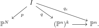
We consider the projection q ̄ : P N × ( P n ) k ( P n ) k . Then a point z P N × ( P n ) k belongs to the indeterminacy locus of ρ 1 if and only if q ̄ ( z ) L ̂ ( i ) for some 𝑖 with 1 i k . Since π R | I ( = π R Seg 1 | I ) coincides with Seg 2 ρ 1 | I , and since R I is the indeterminacy locus of π R | I , we have

R I = q 1 ( i = 1 k L ̂ ( i ) ) ,

where 𝑞 is equal to q ̄ | I : I ( P n ) k . In particular, since the dimension of the fibers of q | I 0 is constant, and since codim ( L ̂ ( i ) , ( P n ) k ) = m + 1 , it follows that codim ( R I 0 , I ) = m + 1 . Now, let { Q s } be the irreducible components of R I . Then codim ( Q s , I ) = m + 1 in the case Q s I 0 , i.e., Q s I I 0 . In order to consider the remaining case Q s I I 0 , we use the irreducible components { W j } of I I 0 . For ( a j , x j , 1 , , x j , k ) W j given in (2.3), since x j , i L ̂ , it follows W j R for any 𝑗.

If an irreducible component Q s of R I satisfies Q s I I 0 , then there is some 𝑗 such that Q s R W j W j I , and then codim ( Q s , I ) 2 . As a result, in any case, each irreducible component of R I is of codimension m + 1 or at least 2, which implies that codim ( R I , I ) 2 .

Now, let ( a , x 1 , , x k ) I I 0 satisfy a P β , where dim x 1 , , x k < k 1 for x i = v d ( x i ) as in Remark 7 (a) (note that we do not know a x 1 , , x k ). We regard ( a , x 1 , , x k ) as a point of P l 1 under the embedding I P l 1 .

If ( a , x 1 , , x k ) R , then

ρ 1 ( a , x 1 , , x k ) = ( a , y 1 , , y 1 )

is determined in ρ 1 ( I ) ̄ P N × ( P m ) k , where y i P m is the image of x i under P n P m . Since a P β ,

ρ 2 ( ρ 1 ( a , x 1 , , x k ) ) = ( a , y 1 , , y 1 )

is determined and is contained in I ( m ) . Then dim y 1 , , y k < k 1 for y i = v d ( y i ) P β , which means ( a , y 1 , , y 1 ) I ( m ) I ( m ) 0 .

Assume ( a , x 1 , , x k ) R . We consider the blowing-up P ̃ l 1 of P l 1 with respect to 𝑅, and the projections r 1 , r 2 in diagram (2.4). Note that, for the strict transformation S P ̃ l 1 of P N × ( P n ) k P l 1 , two composite morphisms

S r 1 | S P N × ( P n ) k P N and S r 2 | S P N × ( P m ) k P N

coincide since it holds on an open subset of 𝑆. Let E P ̃ l 1 be the exceptional divisor, and let I ̃ P ̃ l 1 be the strict transformation of I P l 1 . Then r 2 ( I ̃ ) = ρ 1 ( I ) ̄ . Let

E 1 = r 1 1 ( a , x 1 , , x k ) ( E I ̃ )

be the fiber of E I ̃ R I at ( a , x 1 , , x k ) . It follows from codim ( R I , I ) 2 that dim ( E 1 ) 1 . Since r 1 1 ( z ) r 2 ( r 1 1 ( z ) ) P l 2 for each z P l 1 , we have dim ( r 2 ( E 1 ) ) 1 . Since the image of r 2 ( E 1 ) under P N × ( P m ) k P N is { a } , there is C ( P m ) k of positive dimension such that r 2 ( E 1 ) = { a } × C P N × ( P m ) k . Since a P β and

ρ 2 ( r 2 ( E 1 ) ) ρ 2 ( r 2 ( I ̃ ) ) = ρ 2 ( ρ 1 ( I ) ) ̄ = I ( m ) ,

we have { a } × C = ρ 2 ( { a } × C ) I ( m ) . ∎

Lemma 10

Lemma 10 (Non-triviality of subsecant varieties)

For an 𝑚-plane L = P m P n , we have

σ k ( v d ( L ) ) σ k 1 ( v d ( P n ) ) σ k 1 ( v d ( L ) ) .

In particular, σ k ( v d ( L ) ) σ k 1 ( v d ( P n ) ) unless σ k 1 ( v d ( L ) ) = σ k ( v d ( L ) ) .

Proof

Let a σ k ( v d ( L ) ) σ k 1 ( v d ( P n ) ) (note that 𝑎 can be in the boundary of σ k 1 ( v d ( P n ) ) ). For a general point b 0 σ k 1 ( v d ( P n ) ) , we take an irreducible curve 𝐶 in σ k 1 ( v d ( P n ) ) such that a , b 0 C . Let π 2 : P N P β be the linear projection in Remark 8 (a), and let C = π 2 ( C ) ̄ P β . Since a P β , we have a = π 2 ( a ) C .

Since b 0 is general, for a general point b C , we have

b x 1 , , x k 1 with x 1 , , x k 1 v d ( P n ) .

Take x i P n with x i = v d ( x i ) . Setting y i = π 2 ( x i ) , we have y i = v d ( y i ) with y i L for each i = 1 , , k 1 as in Remark 8 (a). Then π 2 ( b ) y 1 , , y k 1 σ k 1 ( v d ( L ) ) . As a result, a C σ k 1 ( v d ( L ) ) and the assertion follows. ∎

Remark 11

We have some consequences of Lemma 10.

(a) (Border rank preserving pair) For any P m P n and for any k , d > 0 , by Lemma 10, we can derive

(2.5) σ k ( v d ( P n ) ) v d ( P m ) = σ k ( v d ( P m ) )

as a set. Since one inclusion is obvious, let us prove σ k ( v d ( P n ) ) v d ( P m ) σ k ( v d ( P m ) ) . Suppose that it does not hold. Then there exists a form f σ k ( v d ( P n ) ) v d ( P m ) with f σ k 0 ( v d ( P m ) ) σ k ( v d ( P m ) ) for some k 0 > k . Then f σ k 0 ( v d ( P m ) ) σ k 0 1 ( v d ( P n ) ) so that f σ k 0 1 ( v d ( P m ) ) by Lemma 10. Similarly, repeating the same “descent” argument, we have f σ k ( v d ( P m ) ) , which is a contradiction. Thus the equality in (2.5) is true.

In other words, for any 𝑑-th Veronese embedding X = v d ( P n ) and the linear span L = v d ( P m ) of any sub-Veronese variety v d ( P m ) , we showed that ( X , L ) is a border rank preserving pair for any k , d > 0 in the terminology of [22, Definition 5.7.3.1] (we would also like to note that [6, Theorem 1.1] can imply the same result for any d k in case of P m P n ).

(b) (Every Σ k , d ( m ) is closed) Recall that the symmetric subspace variety Sub m ( S d V ) (see [22, Section 7.1.3]) is defined as

{ f P S d V there exists W V such that dim W = m + 1 , f P S d W } .

Let n = dim P V . For any m n , we have Sub m ( S d V ) = P m P V v d ( P m ) . Now, we show that Σ k , d ( m ) is the intersection of the whole 𝑘-th secant σ k ( v d ( P V ) ) and the symmetric subspace variety Sub m ( S d V ) set-theoretically. See that

σ k ( v d ( P V ) ) Sub m ( S d V ) = σ k ( v d ( P V ) ) P m P V v d ( P m ) = P m P V ( σ k ( v d ( P V ) ) v d ( P m ) ) = P m P V σ k ( v d ( P m ) ) ( = Σ k , d ( m ) ) by ( 2.5 ) .

Therefore, we obtain that Σ k , d ( m ) = σ k ( v d ( P V ) ) Sub m ( S d V ) as a set and in particular every 𝑚-subsecant Σ k , d ( m ) is a Zariski-closed locus in σ k ( v d ( P V ) ) .

2.2 General secant fiber of a subsecant variety, entry locus, and its Veronese image

We take another incidence variety J P β × ( Z ) k for an 𝑚-dimensional projective variety Z P β to be the Zariski closure of

(2.6) J 0 = { ( a , x 1 , , x k ) a x 1 , , x k and dim x 1 , , x k = k 1 } ,

with the projections

p : J σ k ( Z ) P β , q i : J ( Z ) k Z ,

where ( Z ) k Z is the projection to the 𝑖-th factor for 1 i k . Then dim J = m k + k 1 for any k dim Z + 1 by considering general fibers of J ( Z ) k .

For a σ k ( Z ) , the scheme-theoretic image q i ( p 1 ( a ) ) in 𝑍 is called the (𝑘-th) entry locus of 𝑍 with respect to 𝑎 in the literature. It is known that, for a general a σ k ( Z ) , the locus q i ( p 1 ( a ) ) is equidimensional, and moreover, if 𝑍 is smooth and in the characteristic 0, then p 1 ( a ) is smooth so that q i ( p 1 ( a ) ) is reduced (see [29, Definition 1.4.5]).

Let Z , X P N be projective varieties of dimensions m , n . Let Z X and Z P β , where P β is a 𝛽-plane of P N (i.e., 𝑍 is degenerate in P N ). Now, a general point a Z does not have to be general in 𝑋 any longer. If β < k m + k 1 , then the projection 𝑝 has positive-dimensional fibers.

We begin with a consequence of Terracini’s lemma in our setting and add two more lemmas concerning “the entry locus” q i ( p 1 ( a ) ) .

Lemma 12

Assume that σ k ( Z ) Sing ( σ k ( X ) ) . Let 𝐹 be an irreducible component of p 1 ( a ) for a general point a σ k ( Z ) in incidence (2.6). Then, for a general point x q i ( F ) with 1 i k , we have T x ( X ) T a ( σ k ( X ) ) where T x ( X ) P N means the embedded tangent space to 𝑋 at 𝑥.

Proof

Since σ k ( Z ) Sing ( σ k ( X ) ) is non-empty open in σ k ( Z ) and 𝑎 is general, it is a smooth point of σ k ( X ) ; hence the embedded tangent space T a ( σ k ( X ) ) is defined. In addition, 𝑎 is contained in the ( k 1 ) -plane x 1 , , x k for general x 1 , , x k Z with x i = x . Then the assertion follows by Terracini’s lemma (cf. [29, Corollary 1.4.2], [30, Chapter II, 1.10, Chapter V, 1.4]). ∎

Lemma 13

For a projective variety 𝑍, let Z = P β and consider the incidence 𝐽 as (2.6) with k 2 . Suppose that the ( k 1 )-secant of 𝑍 is not defective and not equal to P β . Then, for a general point ( a , x 1 , , x k ) J and for any irreducible component 𝐹 of p 1 ( a ) containing ( a , x 1 , , x k ) , q i | F : F q i ( F ) is generically finite.

Proof

For simplicity, we set i = 1 . First, since ( a , x 1 , , x k ) is a general point of the incidence 𝐽, we may assume that 𝑎 is a general point of σ k ( Z ) and x 1 , , x k are 𝑘 general points on 𝑍.

Let π x 1 : P β P β 1 be the linear projection from x 1 . Since 𝑍 is non-degenerate in P β and σ k 1 ( Z ) P β , the map π x 1 | σ k 1 ( Z ) is generically finite onto its image (otherwise, a general point x 1 is contained in Vertex ( σ k 1 ( Z ) ) , a linear subvariety of σ k 1 ( Z ) , a contradiction).

Let J P β × ( Z ) k 1 be the incidence for the ( k 1 ) -secant of 𝑍, i.e., the closure of

{ ( b , x ̃ 2 , , x ̃ k ) b x ̃ 2 , , x ̃ k and dim x ̃ 2 , , x ̃ k = k 2 } .

Since σ k 1 ( Z ) is not secant defective, the first projection p J : J σ k 1 ( Z ) is generically finite. Hence the composite map

(2.7) ρ = π x 1 p J : J π x 1 ( σ k 1 ( Z ) )

is generically finite.

Let J 1 = q 1 1 ( x 1 ) J . Then

π x 1 p | J 1 : J 1 π x 1 ( σ k 1 ( Z ) )

is dominant (this is because, for general b σ k 1 ( Z ) , we take a general point c x 1 , b and k 1 points x ̃ 2 , , x ̃ k Z such that b x ̃ 2 , , x ̃ k ; then ( c , x 1 , x ̃ 2 , , x ̃ k ) J 1 , whose image under π x 1 p is π x 1 ( c ) = π x 1 ( b ) ). Since ( a , x 1 , , x k ) J 1 is general in 𝐽 and by the dominance of π x 1 p | J 1 , we may consider α = π x 1 ( a ) as a general point in π x 1 ( σ k 1 ( Z ) ) .

Let 𝐹 be an irreducible component of p 1 ( a ) containing ( a , x 1 , x 2 , , x k ) , and suppose that q 1 | F has general fibers of positive dimensions. Then the fiber of q 1 | F at x 1 q 1 ( F ) , F J 1 , is of positive dimension, which means that we have ( a , x 1 , x ̃ 2 , , x ̃ k ) F J 1 for fixed a , x 1 and moving ( x ̃ 2 , , x ̃ k ) with positive dimension.

For general ( a , x 1 , x ̃ 2 , , x ̃ k ) F J 1 , we have the intersection point b ( x ̃ 2 , , x ̃ k ) of the line a , x 1 and the hyperplane x ̃ 2 , , x ̃ k in x 1 , x ̃ 2 , , x ̃ k = P k 1 . Note that

π x 1 ( b ( x ̃ 2 , , x ̃ k ) ) = π x 1 ( a ) = α .

The 𝑘-tuple ( b ( x ̃ 2 , , x ̃ k ) , x ̃ 2 , , x ̃ k ) moves with positive dimension since so does ( k 1 )-tuple ( x ̃ 2 , , x ̃ k ) . In other words, the following locus is of positive dimension:

{ ( b ( x ̃ 2 , , x ̃ k ) , x ̃ 2 , , x ̃ k ) ( a , x 1 , x ̃ 2 , , x ̃ k ) F J 1 } ρ 1 ( α ) J ,

which contradicts that 𝜌, given in (2.7), is generally finite. ∎

Lemma 14

For a projective variety Z Z = P β , suppose that σ k 1 ( Z ) is a hypersurface in P β and σ k ( Z ) = P β . Then we have q i ( p 1 ( a ) ) = Z for a general point a σ k ( Z ) . In particular, there is an irreducible component 𝐹 of p 1 ( a ) such that q i ( F ) = Z .

Proof

Since p 1 ( a ) is invariant under permuting x i -factors, we set i = 1 for simplicity. Take a general a σ k ( Z ) = P β . Since Vertex ( σ k 1 ( Z ) ) is a linear subvariety of σ k 1 ( Z ) P β and 𝑍 is non-degenerate in P β , Vertex ( σ k 1 ( Z ) ) Z Z . This implies that, for general x Z , dim x , σ k 1 ( Z ) > dim ( σ k 1 ( Z ) ) so that x , σ k 1 ( Z ) = P β . Thus any given general point a P β sits on a line x , b for any general x Z and for some general b σ k 1 ( Z ) . Taking k 1 points x ̃ 2 , , x ̃ k Z such that b x ̃ 2 , , x ̃ k , we have ( a , x , x ̃ 2 , , x ̃ k ) p 1 ( a ) , which means q 1 ( p 1 ( a ) ) = Z . ∎

Now let us focus on the case

Z = v d ( P m ) P β = ( m + d m ) 1 ,

the image of the 𝑑-uple Veronese embedding of P m . Here we prove a very useful proposition, which is of independent interest itself. In Proposition 15, we consider the entry locus of a general point in 𝑍 and estimate the dimension of the linear span of its image under ( d 1 )-uple Veronese embedding v d 1 : P m P β d 1 = ( m + d 1 m ) 1 .

Proposition 15

Let Z = v d ( P m ) P β with d 3 , 2 m k 2 , and

β = ( m + d m ) 1 < k m + k 1 .

Assume dim ( σ k 1 ( Z ) ) = ( k 1 ) m + k 2 < β (in other words, the ( k 1 )-th secant of 𝑍 is not defective and not equal to P β ), where ( k 1 ) m + k ( m + d m ) . Let J P β × ( Z ) k be the Zariski closure of incidence (2.6), let ( a , x 1 , , x k ) J be a general point, and let F J be an irreducible component of p 1 ( a ) containing ( a , x 1 , , x k ) . Then the following holds.

  1. If ( k 1 ) m + k < ( m + d m ) , then we have

    dim v d 1 ( A ) k + ( k m + k 1 ) dim σ k ( Z )

    for the preimage A P m of q i ( F ) { x 1 , , x k } Z under v d : P m Z and for each 1 i k .

  2. If ( k 1 ) m + k = ( m + d m ) , then q i ( F ) = Z . In addition, if ( d , m ) ( 3 , 2 ) , then

    dim v d 1 ( P m ) k + m .

Remark 16

(a) Two inequalities

β = ( m + d m ) 1 < k m + k 1 and ( k 1 ) m + k ( m + d m )

are equivalent to

( m + d m ) m + 1 < k < ( m + d m ) m + 1 + 1 ;

this occurs if and only if

( m + d m ) m + 1 N and k = ( m + d m ) m + 1 .

(b) In Proposition 15 (ii), if ( d , m ) = ( 3 , 2 ) , then the condition ( k 1 ) m + k = ( m + d m ) gives k = 4 . In this case, q i ( F ) = Z is still true (e.g., by Lemma 13), but

dim v d 1 ( P m ) = dim v 2 ( P 2 ) = 5

is k + m 1 , not greater than or equal to k + m .

To prove Proposition 15, we settle two lemmas, Lemmas 17 and 19; the former one is technical and the latter geometric.

Lemma 17

Let d , m , k be integers such that d 3 and 2 m k 2 .

  1. If ( k 1 ) m + k < ( m + d m ) < k m + k , then ( m + d 1 m ) 1 2 m k 0 .

  2. If ( k 1 ) m + k = ( m + d m ) and ( d , m ) ( 3 , 2 ) , then ( m + d 1 m ) 1 m k 0 .

  3. If ( m + d m ) = k m + k , then ( m + d 1 m ) 1 m k 0 .

Note that Lemma 17 (iii) is applied in a discussion of the proof of Theorem 2 (ii), though it is not used in this section.

To show the lemma, we need some calculations as follows.

Remark 18

(a) Let m = 2 and k m + k > ( m + d m ) . Then ( k 1 ) m + k < ( m + d m ) does not occur. Otherwise, we have

3 k 2 < ( m + d m ) = ( d + 2 ) ( d + 1 ) 2 < 3 k ,

and then ( d + 2 ) ( d + 1 ) 2 = 3 k 1 . Considering the congruence modulo 3, we have

( d + 2 ) ( d + 1 ) 6 k 2 1 ( mod 3 ) .

Then the possible values of ( d + 2 ) ( d + 1 ) are

( d + 2 ) ( d + 1 ) { 2 1 2 ( d = 0 ) , 0 2 0 ( d = 1 ) , 1 0 0 ( d = 2 ) ,

modulo 3, which is absurd.

(b) For d = 3 , 4 , 5 , we calculate numbers 𝑚 satisfying the conditions

( m + d m ) m + 1 N , k = ( m + d m ) m + 1 , and ( k 1 ) m + k < ( m + d m ) .

For d = 3 , the smallest 𝑚 is 5. For d = 4 , the smallest 𝑚 is 3 and the next smallest 𝑚 is 7. For d = 5 , the smallest 𝑚 is 9. The explicit values of δ = ( m + d 1 m ) ( 1 + k + 2 m ) for them are obtained as follows:

( d , m , k , δ ) = ( 3 , 5 , 10 , 0 ) , ( 4 , 3 , 9 , 4 ) , ( 4 , 7 , 42 , 63 ) , ( 5 , 9 , 201 , 495 ) .

Proof of Lemma 17

(i) From Remark 18 (a), we may assume m 3 . Let

δ = ( m + d 1 m ) ( 1 + k + 2 m ) .

Since

( m + d 1 m ) = d m + d ( m + d m ) ,

using ( k 1 ) m + k + 1 ( m + d m ) , we have

δ = ( m + d 1 m ) ( 1 + k + 2 m ) 1 m + d ( d ( ( k 1 ) m + k + 1 ) ( m + d ) ( 1 + k + 2 m ) ) .

Setting k = m + a with a 2 , we have

(2.8) d ( ( k 1 ) m + k + 1 ) ( m + d ) ( 1 + k + 2 m ) = m ( k ( d 1 ) 3 d 1 2 m ) = m ( ( m + a ) ( d 1 ) 3 d 1 2 m ) m ( ( m + 2 ) ( d 1 ) 3 d 1 2 m ) = m ( d m 3 m d 3 ) = m ( ( d 3 ) ( m 1 ) 6 ) .

Then δ 0 holds in the following three cases: d 6 and m 3 ; d = 5 and m 4 ; or d = 4 and m 7 . In addition, in Remark 18 (b) (see also Remark 16 (a)), we explicitly check that δ 0 if d = 4 and m 6 , and that there is no 𝑘 in our range if d = 5 and m = 3 .

On the other hand, when d = 3 , (2.8) implies

d ( ( k 1 ) m + k + 1 ) ( m + d ) ( 1 + k + 2 m ) = m ( 2 ( m + a ) 10 2 m ) = m ( 2 a 10 ) .

Hence δ 0 holds if d = 3 and a 5 . For d = 3 and k = m + a with a = 2 , 3 , 4 , we have

δ = m 2 m 2 k 2 = m ( m 3 ) 2 a 2 > 0

if m 5 . In addition, in Remark 18 (b), we explicitly check that there is no 𝑘 in our range if d = 3 and m 4 .

(ii) Let δ = ( m + d 1 m ) ( 1 + k + m ) . As in (i), using ( k 1 ) m + k = ( m + d m ) , we have

δ = ( m + d 1 m ) ( 1 + k + m ) = 1 m + d ( d ( ( k 1 ) m + k ) ( m + d ) ( 1 + k + m ) ) ,

and

d ( ( k 1 ) m + k ) ( m + d ) ( 1 + k + m ) = k m ( d 1 ) 2 d m m m 2 d ( m + 2 ) m ( d 1 ) 2 d m m m 2 d = ( d 2 ) ( m 2 1 ) 2 3 m .

If d 3 and m 4 , then since ( d 2 ) ( m 2 1 ) 2 3 m m ( m 3 ) 3 1 , it holds δ 0 . If d 4 and m = 3 , then since ( d 2 ) ( m 2 1 ) 2 3 m 5 , it similarly holds δ 0 . On the other hand, if d = 3 and m = 3 , then ( k 1 ) m + k = ( m + d m ) implies

4 k 3 = ( d + 3 ) ( d + 2 ) ( d + 1 ) 3 ! = 20 ;

this case does not occur since 𝑘 cannot be an integer. If d 4 and m = 2 , then

3 k 2 = ( d + 2 ) ( d + 1 ) 2 .

In this case, δ = ( d + 1 ) d 2 k 3 0 , because of

3 ( ( d + 1 ) d 2 k 3 ) 3 ( d + 1 ) d 2 ( d + 2 ) ( d + 1 ) 2 11 = d 2 12 4 .

(iii) Next, we assume ( m + d m ) = k m + k . Then

δ = ( m + d 1 m ) ( 1 + k + m ) = 1 m + d ( d ( k m + k ) ( m + d ) ( 1 + k + m ) ) .

Using k = m + a = ( m + 1 ) + ( a 1 ) with a 2 , we have

d ( k m + k ) ( m + d ) ( 1 + k + m ) = ( d 1 ) k m ( m + d ) ( m + 1 ) = ( d 1 ) m ( m + 1 ) + ( d 1 ) m ( a 1 ) ( m + d ) ( m + 1 ) = ( m + 1 ) ( ( d 1 ) m ( m + d ) ) + ( d 1 ) m ( a 1 ) = ( m + 1 ) ( ( d 2 ) ( m 1 ) 2 ) + ( d 1 ) m ( a 1 ) .

If d 3 , m 2 , and ( d , m ) ( 3 , 2 ) , then we have δ 0 . If ( d , m ) = ( 3 , 2 ) , then since

( m + 1 ) ( ( d 2 ) ( m 1 ) 2 ) + ( d 1 ) m ( a 1 ) = 3 + 4 ( a 1 ) 1 ,

we also have δ 0 . ∎

The next lemma concerns a general fact on linear sections of Veronese varieties, which is of independent interest itself.

Lemma 19

Let k , m 2 . Let x 1 , , x k P m be 𝑘 general points, let

v e : P m P β e = ( m + e m ) 1

be the 𝑒-uple Veronese embedding of P m , and let M = v e ( x 1 ) , v e ( x 2 ) , , v e ( x k ) P β e . Then, for any 𝑘-plane R P β e containing the ( k 1 ) -plane 𝑀, the following holds.

  1. Assume k β e m , and assume that there is a curve C R v e ( P m ) passing through v e ( x 1 ) . Then it holds that

    (2.9) R v e ( x 2 ) , , v e ( x k ) , T v e ( x 1 ) v e ( P m ) .

  2. Assume e 3 and k β e 2 m . Then we have

    dim v e ( x 1 ) ( R v e ( P m ) ) = 0 ,

    where the left-hand side means dimension of component(s) passing through v e ( x 1 ) . In particular, the set of a point { v e ( x 1 ) } is an irreducible component of R v e ( P m ) .

  3. Assume e = 2 and k 1 β 2 2 m . Assume that there is a curve C R v 2 ( P m ) such that v 2 ( x 1 ) C . Then, for any irreducible subset D R v 2 ( P m ) , it holds that D v 2 ( x 1 , x l ) for some l = 2 , , k , where v 2 ( x 1 , x l ) is a conic curve in P β 2 given as the image of the line x 1 , x l P m ,

Proof

Let C R v e ( P m ) be a curve passing through v e ( x 1 ) . Let

π = π v e ( x 2 ) , , v e ( x k ) : P β e P β e k + 1

be the linear projection from the ( k 2 )-plane v e ( x 2 ) , , v e ( x k ) . If k β e m , then the generalized trisecant lemma [29, Proposition 1.4.3] implies

M v e ( P m ) = { v e ( x 1 ) , v e ( x 2 ) , , v e ( x k ) } .

In particular, dim ( M v e ( P m ) ) = 0 and C M . We have π ( v e ( x 1 ) ) π ( C ) ̄ P β e k + 1 because of v e ( x 1 ) C . If 𝐶 is contracted to a point under 𝜋, then π ( C ) ̄ = π ( v e ( x 1 ) ) , which means that C M , a contradiction. Hence π ( C ) ̄ must be a curve.

For the 𝑘-plane R P β e , which contains the ( k 2 )-dimensional center of 𝜋, the image π ( R ) ̄ is a line in P β e k + 1 . Thus π ( C ) ̄ = π ( R ) ̄ . Moreover, it follows

π ( C ) ̄ = π ( R ) ̄ = T π ( v e ( x 1 ) ) π ( R ) ̄ T π ( v e ( x 1 ) ) π ( v e ( P m ) ) ̄ ,

where, by generic smoothness, the right-hand side is equal to π ( T v e ( x 1 ) v e ( P m ) ) since x 1 P m is general. It follows that 𝑅 is contained in the preimage of π ( T v e ( x 1 ) v e ( P m ) ) , which implies inclusion (2.9) of (i).

The condition k β e m holds if 𝑘 or k 1 is at most β e 2 m . Next, we consider a tangential projection

π T v e ( x 1 ) v e ( P m ) : P β e P β e m 1

from the 𝑚-plane T v e ( x 1 ) v e ( P m ) P β e , and its restriction π ̃ = π T v e ( x 1 ) v e ( P m ) | v e ( P m ) on v e ( P m ) . Note that the Veronese variety v e ( P m ) and any embedded tangent space to v e ( P m ) intersect only at one point; in particular, v e ( P m ) T v e ( x 1 ) v e ( P m ) = { v e ( x 1 ) } . If R P β satisfies (2.9), we have

(2.10) π ̃ ( R v e ( P m ) ) π ̃ ( v e ( P m ) ) π ̃ ( v e ( x 2 ) ) , , π ̃ ( v e ( x k ) ) .

By Terracini’s lemma, for general z v e ( P m ) , the linear variety T v e ( x 1 ) v e ( P m ) , T z v e ( P m ) coincides with an embedded tangent space to σ 2 ( v e ( P m ) ) and is of dimension dim σ 2 ( v e ( P m ) ) . Then

π T v e ( x 1 ) v e ( P m ) ( T z v e ( P m ) ) = T π ̃ ( z ) π ̃ ( v e ( P m ) ) P β e m 1

is of dimension dim σ 2 ( v e ( P m ) ) m 1 . It follows

(2.11) dim π ̃ ( v e ( P m ) ) = dim σ 2 ( v e ( P m ) ) m 1 .

Let e 3 and k β e 2 m . Suppose that dim v e ( x 1 ) ( R v e ( P m ) ) > 0 , which means the existence of a curve 𝐶 satisfying condition (i). Since

codim ( π ̃ ( v e ( P m ) ) , P β e m 1 ) ( k 1 ) ( β e 2 m 1 ) ( k 1 ) 0 ,

again the trisecant lemma implies that the right-hand side in (2.10) is only the set of k 1 points π ̃ ( v e ( x 2 ) ) , , π ̃ ( v e ( x k ) ) . Thus each irreducible subset D R v e ( P m ) satisfies

(2.12) π ̃ ( D ) = π ̃ ( v e ( x l ) )

for some l = 2 , , k . (At least, taking D = C , we exactly have (2.12).) From e 3 , we have dim σ 2 ( v e ( P m ) ) = 2 m + 1 (i.e., non-defective). In this case, by (2.11), dim π ̃ ( v e ( P m ) ) = m , i.e., the map π ̃ must be generically finite. Then we reach a contradiction since v e ( x l ) is a general point. This implies that dim v e ( x 1 ) ( R v e ( P m ) ) = 0 .

Finally, we consider the case of e = 2 . Then dim σ 2 ( v 2 ( P m ) ) = 2 m for m 2 (i.e., defective), and by (2.11), dim π ̃ ( v 2 ( P m ) ) = m 1 . This means that the tangential projection π ̃ : v 2 ( P m ) π ̃ ( v 2 ( P m ) ) has fibers of dimension 1. Moreover, as in Remark 8 (a), we know that

π T v 2 ( x 1 ) v 2 ( P m ) : P β 2 = ( m + 2 ) ( m + 1 ) 2 1 P β 2 m 1 = ( m + 1 ) m 2 1

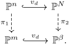
satisfies the commutative diagram

where π x 1 : P m P m 1 is the linear projection from x 1 , and v 2 : P m 1 P ( m + 1 ) m 2 1 is the Veronese embedding of P m 1 . Then

dim ( π ̃ ( v 2 ( P m ) ) ) = dim ( v 2 ( P m 1 ) ) = m 1 .

If k 1 β 2 2 m , then

codim ( π ̃ ( v 2 ( P m ) ) , P β 2 m 1 ) ( k 1 ) ( β 2 2 m ) ( k 1 ) 0 ;

hence the trisecant lemma implies π ̃ ( D ) = π ̃ ( v 2 ( x l ) ) for some l = 2 , , k as we discussed for (2.12).

In the diagram above, for any y x 1 , x l P m with y x 1 , we have

π ̃ ( v 2 ( y ) ) = v 2 ( π x 1 ( y ) ) = v 2 ( π x 1 ( x l ) ) = π ̃ ( v 2 ( x l ) ) ;

indeed,

π ̃ 1 ( π ̃ ( v 2 ( x l ) ) ) = v 2 ( x 1 , x l ) .

Since π ̃ ( D ) = π ̃ ( v 2 ( x l ) ) , we have D v 2 ( x 1 , x l ) . ∎

We give one calculation before proving Proposition 15.

Remark 20

For d = 3 and m 2 , if

μ 0 = ( m + d m ) m + 1 N and k = μ 0

(as under the conditions of Proposition 15 and Remark 16 (a)), then ( k m + k 1 ) β d 1 . The reason is as follows. First, we may write μ 0 = ( m + 3 ) ( m + 2 ) / 6 = M / 3 for some M N since ( m + 3 ) ( m + 2 ) is divisible by 2. In addition, dividing 𝑀 by 3 with remainder, we have M = 3 Q + R for a quotient 𝑄 and a remainder 𝑅. Since μ 0 = M / 3 N , 𝑅 must be 1 or 2. In this setting, k = M / 3 = Q + 1 . It follows that ( k m + k 1 ) β d is equal to

( k m + k ) ( m + 3 3 ) = ( m + 1 ) ( k ( m + 3 ) ( m + 2 ) 6 ) = ( m + 1 ) ( ( Q + 1 ) ( Q + R 3 ) ) = ( m + 1 ) 3 R 3 .

If ( k m + k 1 ) β d = 1 , then 3 = ( m + 1 ) ( 3 R ) . Since 3 R is 1 or 2 and m N , we get m = 2 .

Proof of Proposition 15

(i) For simplicity, we set i = 1 ; then

x 1 q 1 ( F ) Z = v d ( P m ) .

For s = dim σ k ( Z ) , an irreducible component 𝐹 of p 1 ( a ) is of dimension

dim J s = ( k m + k 1 ) s .

From Lemma 13, we have dim q 1 ( F ) = ( k m + k 1 ) s .

Let q 1 ( F ) P m be the preimage of q 1 ( F ) Z under v d : P m Z , and let

A = q 1 ( F ) { x 1 , , x k } P m .

Let v d 1 : P m P β d 1 be the ( d 1 )-uple Veronese embedding. Then the ( k 1 )-plane

v d 1 ( x 1 ) , , v d 1 ( x k ) P β d 1

is contained in the linear variety

v d 1 ( A ) = v d 1 ( q 1 ( F ) ) { v d 1 ( x 1 ) , , v d 1 ( x k ) }

and is of codimension c = dim v d 1 ( A ) ( k 1 ) . By Lemma 17 (i), β d 1 2 m k 0 . So, by the generalized trisecant lemma,

v d 1 ( P m ) v d 1 ( x 1 ) , , v d 1 ( x k ) = { v d 1 ( x 1 ) , , v d 1 ( x k ) } .

In particular,

v d 1 ( q 1 ( F ) ) v d 1 ( x 1 ) , , v d 1 ( x k ) { v d 1 ( x 1 ) , , v d 1 ( x k ) } .

Since dim q 1 ( F ) 1 , we may take a point y q 1 ( F ) such that

v d 1 ( y ) v d 1 ( x 1 ) , , v d 1 ( x k ) .

Assume d 4 . Applying Lemma 19 (ii) to

R = v d 1 ( x 1 ) , , v d 1 ( x k ) , v d 1 ( y ) v d 1 ( A ) ,

we have

dim v d 1 ( x 1 ) ( R v d 1 ( P m ) ) = 0 .

In particular, we have dim v d 1 ( x 1 ) ( R v d 1 ( q 1 ( F ) ) ) = 0 . Regarding it as an intersection of two irreducible subvarieties in v d 1 ( A ) , we deduce that every irreducible component of R v d 1 ( q 1 ( F ) ) is of dimension at least dim ( v d 1 ( q 1 ( F ) ) ) ( c 1 ) . Hence

dim ( v d 1 ( A ) ) k + dim ( v d 1 ( q 1 ( F ) ) ) = k + ( k m + k 1 ) s .

Next, let us consider the case of d = 3 . For l = 2 , , k , since v 2 ( x 1 , x l ) P β 2 is a conic, it follows that v 2 ( x 1 , x l ) is a 2-plane, which is equal to v 2 ( x 1 ) , v 2 ( x l ) , z for some z P β 2 . Then

v 2 ( x 1 ) , , v 2 ( x k ) , v 2 ( x 1 , x l ) = v 2 ( x 1 ) , , v 2 ( x k ) , z

is a linear subvariety of dimension at most 𝑘. Since v 2 ( q 1 ( F ) ) v 2 ( x 1 ) , , v 2 ( x k ) is empty or is a set of points, the intersection

v 2 ( q 1 ( F ) ) v 2 ( x 1 ) , , v 2 ( x k ) , v 2 ( x 1 , x l )

is of dimension at most 1. On the other hand, since m 2 by Remark 18 (a), we have

dim q 1 ( F ) = ( k m + k 1 ) β 2

as in Remark 20. For the union

W = l = 2 , , k v 2 ( q 1 ( F ) ) v 2 ( x 1 ) , , v 2 ( x k ) , v 2 ( x 1 , x l ) P β 2 ,

we see that q 1 ( F ) v 2 1 ( W ) and may take y q 1 ( F ) v 2 1 ( W ) .

Let R = v 2 ( x 1 ) , , v 2 ( x k ) , v 2 ( y ) v 2 ( A ) and suppose that

dim v 2 ( x 1 ) ( R v 2 ( q 1 ( F ) ) ) > 0 ,

that is to say, there is a curve C R v 2 ( q 1 ( F ) ) containing v 2 ( x 1 ) . Taking D = C and applying Lemma 19 (iii), we have C = v 2 ( x 1 , x l ) for some l > 1 . If

dim v 2 ( x 1 ) , , v 2 ( x k ) , v 2 ( x 1 , x l ) = k ,

then R = v 2 ( x 1 ) , , v 2 ( x k ) , v 2 ( x 1 , x l ) , contradicting the definition of 𝑊 and our choice of y . Else, if

dim v 2 ( x 1 ) , , v 2 ( x k ) , v 2 ( x 1 , x l ) = k 1 ,

then C = v 2 ( x 1 , x l ) v 2 ( q 1 ( F ) ) v 2 ( x 1 ) , , v 2 ( x k ) , also contradicting that the intersection is of dimension at most 0.

Hence dim v 2 ( x 1 ) ( R v 2 ( q 1 ( F ) ) ) = 0 . Then, in the same way as above, we have

dim ( v 2 ( A ) ) k + ( k m + k 1 ) s .

(ii) In the case when

( k 1 ) m + k = ( m + d m ) ,

we have k m + k 1 s m . It follows from Lemma 13 and P m Z that q i ( F ) = Z . From Lemma 17 (ii), if ( d , m ) ( 3 , 2 ) , then we have that P β d 1 = v d 1 ( P m ) is of dimension at least k + m . ∎

We end this subsection by making one more important remark on the case when

σ k ( v d ( P m ) ) P β d

is secant defective, which will be used in the proof of Theorem 3 (ii).

Remark 21

Remark 21 (Estimate in defective cases)

For four defective cases

( k , d , m ) = ( 7 , 3 , 4 ) , ( 5 , 4 , 2 ) , ( 9 , 4 , 3 ) , ( 14 , 4 , 4 ) ,

similarly to Proposition 15, we can have an estimation

dim v d 1 ( A ) k + δ ,

where A = v d 1 ( q 1 ( p 1 ( a ) ) ) P m , the preimage of the entry locus of 𝑎, and 𝛿 is the secant defect of σ k ( v d ( P m ) ) ; here 𝐴 is 𝛿-equidimensional, the 𝑘 general points x 1 , , x k P m are contained in 𝐴, and it is well known that δ = 2 when ( k , d , m ) = ( 9 , 4 , 3 ) and δ = 1 in all the other defective cases.

For three cases

( k , d , m ) = ( 5 , 4 , 2 ) , ( 9 , 4 , 3 ) , ( 14 , 4 , 4 ) ,

we see that β d 1 2 m k and

v d 1 ( A ) v d 1 ( x 1 ) , , v d 1 ( x k ) { v d 1 ( x 1 ) , , v d 1 ( x k ) }

by the trisecant lemma so that we may take y A such that

v d 1 ( y ) v d 1 ( x 1 ) , , v d 1 ( x k ) .

By Lemma 19 (ii), we get

dim v d 1 ( x 1 ) ( R v d 1 ( P m ) ) = 0 ,

where

R = v d 1 ( x 1 ) , , v d 1 ( x k ) , v d 1 ( y ) .

Thus, by the intersection argument in v d 1 ( A ) (similar to Proposition 15 (i)), we derive the estimation

dim v d 1 ( A ) dim R + dim v d 1 ( A ) = k + δ .

For the remaining case ( k , d , m ) = ( 7 , 3 , 4 ) , it holds β d 1 2 m = k 1 , and we still can claim that

dim ( v 2 ( A ) ) k + δ = 7 + 1 = 8

as follows. For the 6-dimensional subspace M = v 2 ( x 1 ) , , v 2 ( x 7 ) v 2 ( A ) , the trisecant lemma implies

M v 2 ( A ) M v 2 ( P 4 ) = { v 2 ( x 1 ) , , v 2 ( x 7 ) } ,

the 0-dimensional intersection. Then dim ( v 2 ( A ) ) 7 (otherwise, we get M = v 2 ( A ) so that M v 2 ( A ) = v 2 ( A ) , a contradiction). Suppose that

dim ( v 2 ( A ) ) = 7 ,

and set R = v 2 ( A ) . We take the irreducible components of the 1-equidimensional closed set 𝐴 as A = j = 1 s A j . Note that v 2 ( A j ) R v 2 ( P m ) . Since x 1 A , there is a curve A j 0 containing x 1 . Taking C = v 2 ( A j 0 ) and applying Lemma 19 (iii), for any 𝑗 with 1 j s , we have v 2 ( A j ) = v 2 ( x 1 , x l j ) for some l j = 2 , , k . This is equivalent to A j = x 1 , x l j , a line in P 4 ; in particular, x 1 A j . In the same way, A j must contain x 1 , , x 7 . But this is a contradiction, because these points are chosen as seven general points in P 4 . Thus it follows that dim ( v 2 ( A ) ) 8 .

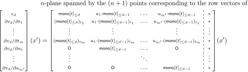
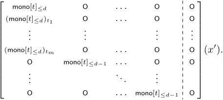
2.3 Estimate for the linear span of tangents moving along a subsecant variety

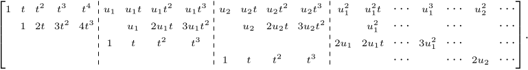
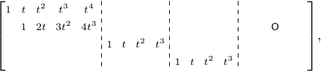
First, we give the following explicit description of the embedded tangent space T x v d ( P n ) P N to v d ( P n ) at a point 𝑥 in v d ( P n ) or v d ( P m ) . Note that it is related to computations of Gauss maps (see [12]).

Recall that mono [ t ] e denotes the set of monomials f C [ t 1 , , t m ] with deg f e . Then 1 mono [ t ] e as the monomial of degree 0. As mentioned in Remark 8, as changing homogeneous coordinates t 0 , t 1 , , t m , u 1 , u 2 , , u m on P n with m = n m , we may assume that P m is the zero set of u 1 , , u m . On the affine open subset { t 0 0 } , the Veronese embedding v d : P n P N is parameterized by monomials of C [ t 1 , , t m , u 1 , , u m ] of degree at most 𝑑. So it is expressed as

(2.13) [ mono [ t ] d : u 1 mono [ t ] d 1 : : u m mono [ t ] d 1 : ] ,

where u i mono [ t ] d 1 means

{ u i f f mono [ t ] d 1 } = ( u i : u i t 1 : u i t 2 : : u i t m d 1 ) ,

and “∗” means the remaining monomials.

Let x = v d ( x ) with x { t 0 0 } P n . Then T x v d ( P n ) P N coincides with the

(2.14)

using (2.13), where ( mono [ t ] e ) t i means { f / t i f mono [ t ] e } and 𝖮 is a zero matrix with suitable size.

In particular, in case of x P m = { u 1 = = u m = 0 } , we see that the matrix is of the form

(2.15)

As a consequence, we settle a key proposition which estimates a lower bound of the dimension of the linear span of moving embedded tangent spaces along a subset of a given P m .

Proposition 22

Let v d : P n P N be the 𝑑-uple Veronese embedding. For an 𝑚-plane P m P n , for a (possibly reducible) subset A P m , and for a linear variety Λ v d ( P m ) , the dimension of the linear variety

Λ x v d ( A ) T x ( v d ( P n ) ) P N

is greater than or equal to

(2.16) dim Λ v d ( A ) + ( n m ) { 1 + dim v d 1 , m ( A ) } ,

where v e , m : P m P ( m + e m ) 1 is the 𝑒-uple Veronese embedding of P m .

Proof

For a given A P m , we consider

B 0 = v d ( A ) , B 1 = ( v d / u 1 ) ( A ) , , B m = ( v d / u m ) ( A )

as subsets in P N , where B i is embedded by the parameterization of the ( m + 1 + i ) -th row of the matrix of (2.14) for 1 i m . Note that, for the homogeneous coordinates [ w 0 : : w N ] on P N corresponding to (2.13), v d ( P m ) = P β = ( m + d m ) 1 is the zero set of w β + 1 , , w N , and Λ B 0 is contained in the set.

Since A { u 1 = = u m = 0 } , it follows from (2.15) that the linear variety

(2.17) Λ B 0 , B 1 , , B m P N

is of dimension dim ( Λ B 0 ) + dim ( B 1 ) + + dim ( B m ) + m .

Again, by (2.15), we see that B 0 v d ( A ) and B i v d 1 , m ( A ) for 1 i m . As the linear variety (2.17) is contained in Λ x v d ( A ) T x ( v d ( P n ) ) , we have the assertion. ∎

3 Case of m = 1

3.1 Symmetric flattening and conormal space computation

For the proof of Theorem 1, we begin with some preliminaries on equations for secant varieties and conormal space computation via known sets of equations, whereas we mainly adopt the geometric viewpoint and techniques for the m 2 case in Section 4.

Let 𝑉 be an ( n + 1 ) -dimensional ℂ-vector space C x 0 , x 1 , , x n . Let f S d V be a homogeneous polynomial of degree 𝑑 (or 𝑑-form) and let [ f ] be the corresponding point in P S d V . In this paper, we frequently abuse notation, denoting both a 𝑑-form in S d V and the point in P S d V just by 𝑓. For the Veronese variety v d ( P V ) , we have a natural one-to-one correspondence between points of the ambient space v d ( P V ) and equivalent classes of degree 𝑑-forms in S = C [ x 0 , x 1 , , x n ] . First of all, let us recall some notions related to this correspondence.

Given a form 𝑓 of degree 𝑑, the minimum number of linear forms l i needed to write 𝑓 as a sum of 𝑑-th powers is the so-called (Waring) rank of 𝑓 and we denote it by rank ( f ) . Note that one can define rank ( [ f ] ) by rank ( f ) , because this rank is invariant under nonzero scaling. The (Waring) border rank is given by the same notion in the limiting sense. In other words, if there is a family { f ϵ ϵ > 0 } of polynomials with constant rank 𝑟 and lim ϵ 0 f ϵ = f , then we say that 𝑓 has border rank at most 𝑟. The minimum such 𝑟 is called the border rank of 𝑓 and we denote it again by rank ¯ ( f ) . Note that, by definition, σ k ( v d ( P V ) ) is the variety of homogeneous polynomials 𝑓 of degree 𝑑 with border rank rank ¯ ( f ) k .

Now, we recall that some part of defining equations for σ k ( v d ( P V ) ) comes from so-called symmetric flattenings. Consider the polynomial ring S = S V = C [ x 0 , , x n ] and consider another polynomial ring T = S V = C [ y 0 , , y n ] , where V is the dualℂ-vector space of 𝑉. Define the differential action of 𝑇 on 𝑆 as follows: for any g T d a , f S d , we set g f = g ( 0 , 1 , , n ) f S a , where i = / x i . Let us take bases for S a and T d a as

X I = 1 i 0 ! i n ! x 0 i 0 x n i n and Y J = y 0 j 0 y n j n ,

with | I | = i 0 + + i n = a , | J | = j 0 + + j n = d a . For a given f = | I | = d b I X I in S d , we have a linear map

ϕ d a , a ( f ) : T d a S a , g g f

for any 𝑎 with 1 a d 1 , which can be represented by the following ( a + n n ) × ( d a + n n ) -matrix:

( b I , J ) with b I , J = b I + J ,

in the bases defined above. We call this “the ( d a , a ) -symmetric flattening (or catalecticant) matrix” of 𝑓. It is easy to see that the transpose ϕ d a , a ( f ) T is equal to ϕ a , d a ( f ) .

It is obvious that if 𝑓 has (border) rank 1, then any symmetric flattening ϕ d a , a ( f ) has rank 1. By subadditivity of matrix rank, we also know that rank ϕ d a , a ( f ) r if rank ¯ ( f ) r . So we obtain a set of defining equations coming from ( k + 1 ) -minors of the matrix ϕ d a , a ( f ) for σ k ( v d ( P V ) ) . For some small values of 𝑘, it is known that these minors are sufficient to cut the variety σ k ( v d ( P V ) ) scheme-theoretically (see [24, Theorem 3.2.1]).

Let us recall some more basic terms and facts. Let Z P W be a (reduced and irreducible) variety and Z ̂ its affine cone in 𝑊. Consider a (closed) point p ̂ Z ̂ and call 𝑝 the corresponding point in P W . We denote the affine tangent space to 𝑍 at 𝑝 in 𝑊 by T ̂ p Z and we define the (affine) conormal space to 𝑍 at 𝑝, N ̂ p Z as the annihilator ( T ̂ p Z ) W . Since dim N ̂ p Z + dim T ̂ p Z = dim W and dim Z dim T ̂ p Z 1 , we get that

(3.1) dim N ̂ p Z codim ( Z , P W )

and the equality holds if and only if 𝑍 is smooth at 𝑝. This conormal space is quite useful to study the (embedded) tangent space T p Z .

For any given form f S d V , we call T t apolar to 𝑓 if the differentiation f gives zero (i.e., ker ϕ t , d t ( f ) ). And we define the apolar ideal f T as

f = { T f = 0 } .

It is straightforward to see that f is indeed an ideal of 𝑇. Moreover, it is well known that the quotient ring T f = T / f is an Artinian Gorenstein algebra with socle degree 𝑑 (see e.g. [19, Chapter 1]). In terms of this apolar ideal, we have a useful description of (a part of) conormal space as follows.

Proposition 23

Suppose that f S d V corresponds to a (closed) point [ f ] of

σ k ( v d ( P V ) ) σ k 1 ( v d ( P V ) ) .

Then, for any 𝑎 with 1 a d + 1 2 with rank ϕ d a , a ( f ) = k , we have

N ̂ [ f ] σ k ( v d ( P V ) ) ( f ) a ( f ) d a

as a subspace of T d = S d V .

Proof

Let X P W be any variety. For any linear embedding W A B and the induced embedding

X P W P ( A B ) ,

it is well known that, for any [ f ] σ k ( X ) P ( A B ) , considering σ k ( X ) as a subvariety of P ( A B ) , we have

N ̂ [ f ] σ k ( X ) ker ( f ) im ( f ) = N ̂ [ f ] σ p ( Seg ( P A × P B ) )

in A B provided that X σ p ( Seg ( P A × P B ) ) , X σ p 1 ( Seg ( P A × P B ) ) and 𝑓 has rank k p as a linear map in Hom ( A , B ) (see e.g. [24, Section 2.5]). Here Seg ( P A × P B ) means the Segre variety in P ( A B ) .

Further, since X P W P ( A B ) , then as a subvariety of P W , it holds that

N ̂ [ f ] σ k ( X ) π ( ker ( f ) im ( f ) ) = N ̂ [ f ] ( σ p ( Seg ( P A × P B ) ) P W ) ,

where π : A B W is the dual map of the given inclusion W A B .

The assertion is immediate when we apply this fact to a partial polarization

S d V S a V S d a V ,

because X = v d ( P V ) is contained in Seg ( P S a V × P S d a V ) P ( S a V S d a V ) (i.e., p = 1 case) and

rank ϕ d a , a ( f ) = k ,
ker ϕ d a , a ( f ) = ( f ) d a ,
im ( ϕ d a , a ( f ) ) = ( f ) a .

3.2 Proof of Theorem 1

Now we study singularity and non-singularity of the subsecant variety σ k ( v d ( P 1 ) ) σ k ( v d ( P n ) ) in each range of k , d as in Theorem 1.

Proof of Theorem 1

(i) Let 𝑓 be any form belonging to σ k ( v d ( P 1 ) ) σ k 1 ( v d ( P n ) ) . Set X = v d ( P n ) P N , the Veronese variety. Consider 𝑓 as a polynomial in C [ x 0 , x 1 ] as in Section 3.1. Then, by [19, Theorem 1.44], we know that T / f is an Artinian Gorenstein algebra with socle degree 𝑑 and that f is a complete intersection of two homogeneous polynomials F , G , each of degree 𝑎 and 𝑏 ( a b ) with a + b = d + 2 , as an ideal of C [ y 0 , y 1 ] , where the Hilbert function of T / f is

(3.2) ( 1 , 2 , , a 1 , a , , a , a 1 , , 2 , 1 ) .

We claim that rank ϕ k , d k ( f ) = k (i.e., a = k ). If a < k , then by shape (3.2), we see that rank ϕ t , d t ( f ) < k for all 𝑡. In particular, all 𝑘-minors of ϕ t , d t ( f ) vanish for any 𝑡. As the 𝑘-minors of catalecticant ϕ t , d t for each k 1 t d ( k 1 ) give the ideal of σ k 1 ( v d ( P 1 ) ) (e.g. [19, Theorem 1.45]), this implies f σ k 1 ( v d ( P 1 ) ) σ k 1 ( v d ( P n ) ) , which is a contradiction. Hence we have that f = ( F , G , y 2 , , y n ) as an ideal in T = C [ y 0 , y 1 , , y n ] for some polynomial 𝐹 of degree 𝑘 and 𝐺 of degree ( d k + 2 ) in C [ y 0 , y 1 ] .

Now, let us show that σ k ( X ) is smooth at 𝑓 by computing the dimension of conormal space. In general, by (3.1), we have

(3.3) ( n + d d ) k n k dim C N ̂ [ f ] σ k ( X ) ,

where the left-hand side is given by the expected codimension of the 𝑘-th secant variety. By Proposition 23, we also have

(3.4) dim C N ̂ [ f ] σ k ( X ) dim C ( f ) k ( f ) d k .

Thus 𝑓 is a smooth point of σ k ( X ) if the lower bound for the dimension of conormal space in (3.4) is equal to the expected codimension in (3.3).

Since k d + 1 2 by the assumption, note that d k k unless 𝑑 is odd and k = d + 1 2 , where d k = d 1 2 < k .

(a) If 𝑑 is odd and k = d + 1 2 , then we have

( f ) k ( f ) d k = ( F , y 2 , , y n ) k ( y 2 , , y n ) d k = ( { y i y j 2 i , j n } ) d ̇ F { y 2 , , y n } { y 0 d k 1 , y 0 d k 2 y 1 , , y 1 d k 1 } = C [ y 0 , y 1 , , y n ] d ( { y 0 d , y 0 d 1 y 1 , , y 1 d } ̇ { y 2 , , y n } { y 0 d 1 , , y 1 d 1 } ) ̇ F { y 2 , , y n } { y 0 d k 1 , y 0 d k 2 y 1 , , y 1 d k 1 } ,

where ̇ means the “disjoint union” of sets of forms of degree 𝑑.

So we obtain

dim N ̂ [ f ] σ k ( X ) dim C ( f ) k ( f ) d k = ( n + d d ) ( d + 1 ) d ( n 1 ) + ( n 1 ) ( d k ) ( note that k = d + 1 2 ) = ( n + d d ) k n k ,

which tells us that σ k ( X ) is smooth at 𝑓.

(b) When 𝑑 is odd and k < d + 1 2 or 𝑑 is even, we have k d k and

( f ) k ( f ) d k = ( F , y 2 , , y n ) k ( F , y 2 , , y n ) d k = ( { y i y j 2 i , j n } ) d ̇ F { y 2 , , y n } { y 0 d k 1 , y 0 d k 2 y 1 , , y 1 d k 1 } ̇ F 2 { y 0 d 2 k , y 0 d 2 k 1 y 1 , , y 1 d 2 k } .

Thus, by a dimension counting similar to case (a), we see that

dim N ̂ [ f ] σ k ( X ) ( n + d d ) ( d + 1 ) d ( n 1 ) + ( n 1 ) ( d k ) + ( d 2 k + 1 ) = ( n + d d ) k n k ,

which coincides with the expected codimension as desired. Thus 𝑓 is a smooth point of σ k ( X ) .

(ii) First note that dim σ k ( v d ( P 1 ) ) = min { 2 k 1 , d } and the incidence 𝐼 has dimension 2 k 1 . In the case d 2 k 2 , each fiber of p : I P d is of dimension at least 1, so for a general a σ k ( v d ( P 1 ) ) , it holds q i ( p 1 ( a ) ) = v d ( P 1 ) for some 𝑖 with 1 i k in incidence (2.6) in Section 2.2.

Now, let n 3 , k = 3 or n 2 , k 4 and d = 2 k 2 . Suppose

σ k ( v d ( P 1 ) ) Sing ( σ k ( v d ( P n ) ) ) .

Then a general point

a σ k ( v d ( P 1 ) ) = P d

is a smooth point of σ k ( v d ( P n ) ) . Since q i ( p 1 ( a ) ) = v d ( P 1 ) for some 𝑖, it follows from Lemma 12 that, for M = T a σ k ( v d ( P n ) ) , we have the inclusion T x ( v d ( P n ) ) M for a general x v d ( P 1 ) , and then the inclusion holds for any x v d ( P 1 ) . This is because, for the Gauss map γ : v d ( P n ) G ( n , P N ) sending γ ( z ) = T z ( v d ( P n ) ) (a morphism since v d ( P n ) is smooth), considering the closed set G M = { W G ( n , P N ) W M } , we have γ ( U ) G M for a certain non-empty open subset U v d ( P 1 ) , and then γ ( v d ( P 1 ) ) G M . Therefore,

(3.5) x v d ( P 1 ) T x ( v d ( P n ) ) T a σ k ( v d ( P n ) ) .

Taking m = 1 , Λ = , and A = P 1 in Proposition 22, the number (2.16), a lower bound for dimension of left-hand side of (3.5), is equal to d n . Thus we have

( 2 k 2 ) n = d n k ( n + 1 ) 1 ( = dim T a σ k ( v d ( P n ) ) ) ,

which is equivalent to the formula n ( k 1 ) / ( k 2 ) . It follows that n 2 if k = 3 , and n = 1 if k 4 , contrary to our assumption.

Finally, since

σ k 1 ( v d ( P 1 ) ) σ k ( v d ( P 1 ) ) when d 2 k 2

(note that dim σ k 1 ( v d ( P 1 ) ) = 2 k 3 < d ), the σ k ( v d ( P 1 ) ) is a non-trivial singular locus of σ k ( v d ( P n ) ) , which means that σ k ( v d ( P 1 ) ) σ k 1 ( v d ( P n ) ) , by Lemma 10.

(iii) By assumption, dim σ k 1 ( v d ( P 1 ) ) = min { 2 k 3 , d } = d , that is to say,

σ k 1 ( v d ( P 1 ) ) = σ k ( v d ( P 1 ) ) = v d ( P 1 ) = P d ;

hence the assertion follows.

(iv) For ( n , k ) = ( 2 , 3 ) , smoothness of all points in σ 3 ( v d ( P 1 ) ) σ 2 ( v d ( P 2 ) ) for d 4 was already proved in [16, Theorem 2.14]. This is included for completeness. ∎

Remark 24

Part (iv) is the exception to the trichotomy in Theorem 1. Under the condition ( k , d , m , n ) = ( 3 , 4 , 1 , 2 ) of (iv), the arithmetic deduced from the inclusion assumption (3.5) of moving tangents in the proof does not make any contradiction. The situation is similar in the other exceptional case to the trichotomy, ( k , d , m , n ) = ( 4 , 3 , 2 , 3 ) (Theorem 2 (iv)).

4 Proof of main results

In this section, we prove Theorems 2 and 3. We will first discuss the non-singularity result and then the results for the singular loci.

4.1 Generic smoothness

We begin with a lemma which deals with a secant fiber of a general point in an 𝑚-subsecant variety v d ( P m ) in v d ( P n ) P N .

Lemma 25

Assume

dim σ k ( v d ( P n ) ) = n k + k 1 and dim σ k ( v d ( P m ) ) = m k + k 1

(i.e., v d ( P n ) and v d ( P m ) are non-defective). Let k ( m + d 1 m ) . Fix L = P m P n to be an 𝑚-plane, and take a σ k ( v d ( L ) ) to be a general point. In the incidence I P N × ( P n ) k with the first projection p : I P N as in (2.1), we then have the following inclusion scheme-theoretically: p 1 ( a ) { a } × ( L ) k .

Proof

(i) Consider any ( a , x 1 , , x k ) p 1 ( a ) I . Let I ( m ) P N × ( L ) k be another incidence as in Lemma 9. Since a σ k ( v d ( L ) ) is general, it follows a σ k 1 ( v d ( L ) ) and a p ( I ( m ) I ( m ) 0 ) by Remark 7 (b). Since dim σ k ( v d ( L ) ) = m k + k 1 , the secant fiber of I ( m ) P N at 𝑎 also consists of finite points. So, by Lemma 9, we have ( a , x 1 , , x k ) I 0 . From Lemma 10, it is also true that a σ k 1 ( v d ( P n ) ) . Thus we may write

a = i = 1 k c i x i for some c i C ,

regarding 𝑎 and x i = v d ( x i ) as vectors in the affine space C N + 1 , where c i 0 for 1 i k .

As in Remark 8, set y i = [ x i , 0 : : x i , m : 0 : : 0 ] . For y i = v d ( y i ) , diagram (2.2) implies

a = i = 1 k c i y i , where y i 0 for 1 i k .

For the affine open subset V 0 = { t 0 0 } P n , we may assume x i V 0 for all 𝑖. Since v d : P n P N is parameterized on V 0 by mono [ t , u ] d , and a v d ( L ) , it holds that

0 = i = 1 k c i { ( u 1 mono [ t ] d 1 ) ( x i ) } = i = 1 k c i x i , m + 1 { mono [ t ] d 1 ( y i ) } ,

where for Mono = u 1 mono [ t ] d 1 , mono [ t ] d 1 and pt = x i , y i , the symbol { Mono ( pt ) } means the vector obtained by evaluating monomials in Mono at the value of pt .

Since k ( m + d 1 m ) , applying Remark 7 (b) to σ k ( v d ( L ) ) , we may assume

(4.1) dim v d 1 ( y 1 ) , , v d 1 ( y k ) = k 1 ,

which gives c i x i , m + 1 = 0 ; thus we have x i , m + 1 = 0 for all 1 i k (more precisely, the linear independence of (4.1) means a 𝑘-minor of the corresponding matrix is nonzero, and c i x i , m + 1 = 0 is obtained by multiplying the inverse of the k × k submatrix). Similarly, we can obtain x i , j = 0 for each j > m and for all 1 i k , which gives the linear defining equations for ( L ) k in ( P n ) k . Hence x 1 , , x k L .

(ii) Let U ( P n ) k be the open subset used in Remark 7, where I 0 is the P k 1 -bundle over 𝑈. We define a morphism Φ : P k 1 × U P N × U by

Φ ( ( c 1 : : c k ) , ( x 1 , , x k ) ) = ( i = 1 k c i v d ( x i ) , ( x 1 , , x k ) ) .

Note that, by the linear independence of v d ( x 1 ) , , v d ( x k ) for ( x 1 , , x k ) U ,

i = 1 k c i v d ( x i ) = i = 1 k c ̃ i v d ( x i ) P N

if and only if ( c 1 : : c k ) = ( c ̃ 1 : : c ̃ k ) P k 1 . Then Φ ( P k 1 × U ) = I 0 , and moreover, we have the isomorphism P k 1 × U I 0 under Φ.

Let U 0 = U ( V 0 ) k ( P n ) k , where ( V 0 ) k is an affine variety and its affine coordinates ring is A = C [ { x i , j } ] . In addition, for each 𝑘-minor 𝜉 of the matrix whose 𝑖-th column consists of monomials of 𝑚 variables x i , 1 , , x i , m of degrees at most d 1 , we set ( V 0 ) ξ k = { ξ 0 } , an open subset of ( V 0 ) k whose coordinates ring is A ξ . Let W { c 1 0 } P k 1 be the affine open subset such that all the coordinates c 1 , , c k are nonzero, where the coordinates ring of 𝑊 is C [ c 2 , , c k ] c 2 c k by regarding c 1 = 1 .

We may assume p 1 ( a ) I 0 ( { a } × ( V 0 ) k ) . To consider the scheme-theoretic structure of p 1 ( a ) , for the composite morphism Φ 1 = p Φ : P k 1 × U 0 P N , we take the fiber

Φ 1 1 ( a ) P k 1 × U 0 P k 1 × ( V 0 ) k .

Since a σ k 1 ( v d ( P n ) ) , Φ 1 1 ( a ) W × ( V 0 ) k . Since 𝑎 is general in σ k ( v d ( L ) ) , and by (4.1), Φ 1 1 ( a ) is contained in the union of affine open subsets W × ( V 0 ) ξ k with all 𝑘-minors 𝜉.

We take

F ξ = Φ 1 1 ( a ) ( W × ( V 0 ) ξ k )

for each 𝜉, and consider the ideal I ( F ξ ) in A ξ [ c 2 , , c k ] c 2 c k , the affine coordinates ring of W × ( V 0 ) ξ k . For β = ( m + d m ) 1 , we may write

a = ( 1 : a ( 1 ) : : a ( β ) : 0 : : 0 ) v d ( L ) P N

with a ( 1 ) , , a ( β ) C and a ( ) = 0 if > β . Then the expression a = i = 1 k c i v d ( x i ) means that

a ( ) i = 1 k c i v d ( x i ) ( 0 ) i = 1 k c i v d ( x i ) ( ) I ( F ξ ) for 1 N ,

where v d ( x i ) ( ) is the ℓ-th coordinate of v d ( x i ) P N . In particular,

i = 1 k c i v d ( x i ) ( ) I ( F ξ ) for > β .

Using the discussion of (i), we have x i , j I ( F ξ ) for all 1 i k and j > m , which means that I ( F ξ ) contains the defining ideal of ( P k 1 × ( L ) k ) ( W × ( V 0 ) ξ k ) . Thus, scheme-theoretically, it follows F ξ P k 1 × ( U 0 ( L ) k ) for any 𝜉, and hence

Φ 1 1 ( a ) P k 1 × ( U 0 ( L ) k ) .

Therefore, p 1 ( a ) { a } × ( L ) k . ∎

Remark 26

We recall some known results on the 𝑘-the secant variety and its incidence in terms of 𝑘-fold symmetric product of P n .

  1. It is known that Sym k ( P n ) is non-singular at ( x 1 , , x k ) if x i x j whenever i j . Thus the subset of all distinct 𝑘-points of P n is a smooth open subscheme of Sym k ( P n ) (see e.g. [4, Lemma 7.1.4]). Then we also consider the incidence variety in this setting as I ̃ P N × Sym k ( P n ) , where I ̃ corresponds to 𝐼 in (2.1) under the natural map P N × ( P n ) k P N × Sym k ( P n ) and p ̃ : I ̃ σ k ( v d ( P n ) ) P N is the first projection.

  2. Assume k ( n + 1 ) < ( n + d n ) . Then we know from [8, Theorem 1.1] that the projection p ̃ : I ̃ σ k ( v d ( P n ) ) is birational except for ( k , d , n ) = ( 9 , 6 , 2 ) , ( 8 , 4 , 3 ) , ( 9 , 3 , 5 ) , because it is a dominant and generically injective morphism.

Now, we are ready to prove Theorem 2 (i) and Theorem 3 (i).

Proof of Theorem 2 (i) and Theorem 3 (i)

For an 𝑚-plane P m P n with m 2 , we take the 𝑚-subsecant variety Z = σ k ( v d ( P m ) ) of Y = σ k ( v d ( P n ) ) . From [2], for d 3 , 𝑍 does not fill Z and is secant defective if and only if

( k , d , m ) = ( 7 , 3 , 4 ) , ( 5 , 4 , 2 ) , ( 9 , 4 , 3 ) , ( 14 , 4 , 4 ) .

Thus, by the assumptions of Theorems 2 and 3, we know that

dim Y = n k + k 1 , dim Z = m k + k 1 dim Z = ( m + d m ) 1 ,

that is, Y , Z are non-defective. In this case, Z = Z if and only if

k = ( m + d m ) m + 1 N .

In particular, under the assumption k < μ of Theorem 2 (i), we have Z Z .

If Z Z , then since ( k , d , m ) = ( 9 , 3 , 5 ) , ( 8 , 4 , 3 ) , ( 9 , 6 , 2 ) are excluded from Theorem 2 and Table 1 (i), it follows from [8, Theorem 1.1] that 𝑍 is generically identifiable. If Z = Z , then ( k , d , m ) = ( 5 , 3 , 3 ) , ( 7 , 5 , 2 ) of Table 1 (i) only occur, and in these cases, it follows from [14, Theorem 1] that 𝑍 is generically identifiable.

Let a Z be a general point and consider p ̃ : I ̃ Y . Note that k ( m + d 1 m ) for each ( k , d , m ) of our range, an assumption of Lemma 25. Applying Lemma 25, Remark 26 (b), and the generic identifiability of 𝑍, we may assume that the scheme-theoretic fiber p ̃ 1 ( a ) is one point x = ( a , x 1 , , x k ) I ̃ ( P N × Sym k ( L ) ) and 𝐱 is a non-singular point in I ̃ , because 𝐱 is contained in a smooth Zariski open subset of I ̃ (i.e., a projective bundle over a smooth open base; see Remarks 7 (a) and 26 (a)).

Now, we restrict the projective morphism p ̃ : I ̃ Y onto a non-empty affine open neighborhood a W = Spec A Y and another open subset x U = Spec B I ̃ , and take the injective ring homomorphism A B corresponding to p ̃ | U : U W . Also, let m a (resp. m x ) be the maximal ideal of 𝑎 in 𝐴 (resp. of 𝐱 in 𝐵). Note that we may take 𝑈 so that p ̃ | U : U W is a finite morphism (cf. [18, Chapter II, Example 3.22 (d)]).

Since A / m a = B / m x C and p ̃ 1 ( a ) Spec ( B A A / m a ) Spec ( B / m a B ) is isomorphic to one simple point Spec B / m x , we have m a B = m x in 𝐵. Let B m a = B A A m a , whose member can be expressed as b / s with b B , s A m a . We have m a B m a = m x B m a in B m a , and then

( A m a + m a B m a ) / m a B m a A m a / m a A m a B m a / m a B m a ,

which implies A m a + m a B m a = B m a + m a B m a = B m a as A m a -module. By the Nakayama lemma (see e.g. [26, Corollary of Theorem 2.2]), it follows A m a = B m a . In particular, B m a is a local ring, whose maximal ideal is m x B m a . Thus we have

A m a = B m a = ( B m a ) m x B m a = B m x ,

which implies that 𝑎 is a smooth point in 𝑌. ∎

We present an example which shows that one cannot extend this generic smoothness result to an arbitrary point in the locus σ k ( v d ( P m ) ) σ k 1 ( v d ( P n ) ) .

Example 27

Example 27 (Singularity can occur at a special point in Theorem 3 (i))

Let

V = C x , y , z , w W = C x , y , z

and let f = x 2 y 2 + z 4 be a form of degree 4. Then 𝑓 represents a point in

σ 4 ( v 4 ( P W ) ) σ 3 ( v 4 ( P V ) ) .

Note that rank ϕ 2 , 2 ( f ) = 4 > 3 , where ϕ a , d a : S d V S a V S d a V is the symmetric flattening. Theorem 3 (i) shows that a general form in σ 4 ( v 4 ( P W ) ) σ 3 ( v 4 ( P V ) ) is a smooth point. But here we show that 𝑓 is a singular point of σ 4 ( v 4 ( P V ) ) . We know that the form f D = x 2 y 2 has Waring rank 3 so that f D = 1 4 + 2 4 + 3 4 for some i C [ x , y ] 1 . By [16, Theorem 2.1], f D is also a singular point of σ 3 ( v 4 ( P V ) ) . Since f f D , z 4 , by Terracini’s lemma, we see that T z 4 v 4 ( P V ) T f σ 4 ( v 4 ( P V ) ) and T i v 4 ( P V ) T f σ 4 ( v 4 ( P V ) ) for any 𝑖. Further, because σ 3 ( v 4 ( P 1 ) ) = v 4 ( P 1 ) and f D has 1-dimensional secant fiber in its incidence, one can move i along this P 1 . Thus we have

(4.2) T f σ 4 ( v 4 ( P V ) ) i P 1 T i 4 v 4 ( P V ) , T z 4 v 4 ( P V ) .

Note that, using parameterization (2.13), we can estimate the dimension of the right-hand side of (4.2). Take an affine open subset { [ 1 : t : u 1 : u 2 ] } of P 3 and (with a change of coordinates) let z 4 be [ 1 : 0 : 1 : 1 ] and let i P 1 be represented by [ 1 : t : 0 : 0 ] for t C . Then, by (2.14), the embedded tangent space to v 4 ( P V ) at [ 1 : t : u 1 : u 2 ] is given as the row span of

On [ 1 : t : 0 : 0 ] (for all t C ), this matrix turns into the shape

and at [ 1 : 0 : 1 : 1 ] , it is equal to

which shows that dim i P 1 T i 4 v 4 ( P V ) 12 , dim T z 4 v 4 ( P V ) = 3 , and

i P 1 T i 4 v 4 ( P V ) T z 4 v 4 ( P V ) = .

Thus, by (4.2), we obtain dim T f σ 4 ( v 4 ( P V ) ) 16 = 12 + 3 + 1 , greater than the expected dimension. Hence 𝑓 is a singular point of σ 4 ( v 4 ( P V ) ) , whereas σ 4 ( v 4 ( P V ) ) is smooth at a general point of σ 4 ( v 4 ( P W ) ) .

4.2 Singularity

In this subsection, we will prove parts (ii) and (iii) both in Theorem 2 and Theorem 3, which show the singularity of the 𝑚-subsecant loci Σ k , d ( m ) in the 𝑘-th secant variety σ k ( v d ( P n ) ) . As Σ k , d ( m ) is the union of all the 𝑚-subsecant varieties σ k ( v d ( P m ) ) in σ k ( v d ( P n ) ) as (1.3), it is enough to prove the statements for any σ k ( v d ( P m ) ) σ k ( v d ( P n ) ) .

Proof of Theorem 2 (ii) and Theorem 3 (ii)

As we noted above, it is enough here to show that σ k ( v d ( P m ) ) Sing ( σ k ( v d ( P n ) ) ) and σ k ( v d ( P m ) ) σ k 1 ( v d ( P n ) ) for each 𝑚-subsecant variety σ k ( v d ( P m ) ) σ k ( v d ( P n ) ) .

We will first prove that σ k ( v d ( P m ) ) Sing ( σ k ( v d ( P n ) ) ) under the condition in Theorem 2 with

( m + d m ) m + 1 N ,

next for Theorem 3 with ( k , d , m ) ( 9 , 3 , 5 ) , ( 8 , 4 , 3 ) , ( 9 , 6 , 2 ) , and finally for

( m + d m ) m + 1 N

or ( k , d , m ) = ( 9 , 3 , 5 ) , ( 8 , 4 , 3 ) , ( 9 , 6 , 2 ) . Basically, we use the same idea for the proof, but a detailed way of estimation will be slightly different according to each case (due to secant defectivity and non-identifiability). The non-triviality of the singular locus, i.e.,

σ k ( v d ( P m ) ) σ k 1 ( v d ( P n ) ) ,

can be directly obtained at the end by Lemma 10.

Take a general point ( a , x 1 , , x k ) in the incidence 𝐽 as (2.6) for Z = v d ( P m ) P β and take an irreducible component 𝐹 of p 1 ( a ) containing ( a , x 1 , , x k ) . Then it follows that a σ k ( v d ( P m ) ) is a general (so smooth) point in σ k ( v d ( P m ) ) .

Suppose σ k ( v d ( P m ) ) Sing ( σ k ( v d ( P n ) ) ) . Then we may assume that 𝑎 is also a smooth point in σ k ( v d ( P n ) ) . In particular, we have

T a ( σ k ( v d ( P m ) ) ) T a ( σ k ( v d ( P n ) ) ) .

Terracini’s lemma implies T x i v d ( P n ) T a σ k ( v d ( P n ) ) for i = 1 , , k , and Lemma 12 implies T x ( v d ( P n ) ) T a ( σ k ( v d ( P n ) ) ) for a general point x q i ( F ) . Thus we have

(4.3) T a ( σ k ( v d ( P m ) ) ) x q i ( F ) { x 1 , , x k } T x ( v d ( P n ) ) T a ( σ k ( v d ( P n ) ) ) .

First of all, let us consider Theorem 2 (ii) with

( m + d m ) m + 1 N .

Set

k = ( m + d m ) m + 1 .

Then

β = ( m + d m ) 1 < k m + k 1 and ( k 1 ) m + k ( m + d m )

as in Remark 16. We have P β = T a ( σ k ( v d ( P m ) ) ) since σ k ( v d ( P m ) ) fills up the whole P β . It is enough to discuss the following three cases:

  1. ( k 1 ) m + k < ( m + d m ) ,

  2. ( k 1 ) m + k = ( m + d m ) and ( d , m ) ( 3 , 2 ) ,

  3. ( k 1 ) m + k = ( m + d m ) and ( d , m ) = ( 3 , 2 ) .

For case (a1) (i.e., ( k 1 ) m + k < ( m + d m ) ), we take A = v d 1 ( q i ( F ) { x 1 , , x k } ) in P m and Λ = P β . From Proposition 15 (i), we get dim v d 1 , m ( A ) k + ( k m + k 1 ) β for the ( d 1 )-uple Veronese embedding v d 1 , m of P m . From Proposition 22, the dimension of the left-hand side in (4.3) is greater than or equal to the number (2.16), which is

dim Λ v d ( A ) + ( n m ) { 1 + dim v d 1 , m ( A ) } β + ( n m ) ( 1 + k + ( k m + k 1 ) β ) .

From inclusion (4.3), we obtain

β + ( n m ) ( 1 + k + ( k m + k 1 ) β ) k n + k 1 ,

which implies ( n m ) ( 1 + ( k m + k 1 ) β ) ( k m + k 1 ) β . This is a contradiction, because n > m and ( k m + k 1 ) β > 0 .

Now, assume ( k 1 ) m + k = ( m + d m ) (equivalently, k m + k 1 β = m ). Then, in the same way as above, using Proposition 15 (ii) and taking

A = P m = v d 1 ( Z ) and Λ = v d ( P m ) = P β ,

we have

(4.4) β + ( n m ) ( 1 + dim v d 1 , m ( P m ) ) k n + k 1 .

For ( d , m ) ( 3 , 2 ) (i.e., case (a2)), Proposition 15 implies that dim v d 1 , m ( P m ) k + m . Then ( n m ) ( m + 1 ) k m + k 1 β = m , contrary to n > m .

For ( d , m ) = ( 3 , 2 ) (i.e., case (a3)), we get β = 9 , dim v d 1 , m ( P m ) = 5 , and

k = ( m + d m ) m + 1 = 4 .

The condition ( k , d , n ) ( 4 , 3 , 3 ) implies n 4 . Then we also have a contradiction since (4.4) does not hold. Hence we show that σ k ( v d ( P m ) ) Sing ( σ k ( v d ( P n ) ) ) .

Secondly, let us regard Theorem 3 (ii). For ( k , d , m ) = ( 10 , 3 , 5 ) , ( 10 , 6 , 2 ) , we have the same result as Theorem 2 since σ k ( v d ( P m ) ) = P β and it satisfies (a1), (a2) respectively. Then, except for ( k , d , m ) = ( 9 , 3 , 5 ) , ( 8 , 4 , 3 ) , ( 9 , 6 , 2 ) , the remaining part of Theorem 3 (ii) consists of the following two cases:

  1. ( k , d , m ) = ( 7 , 3 , 4 ) , ( 5 , 4 , 2 ) , ( 9 , 4 , 3 ) , ( 14 , 4 , 4 ) (i.e., the case of σ k ( v d ( P m ) ) being defective),

  2. ( k , d , m ) = ( 8 , 3 , 4 ) , ( 6 , 4 , 2 ) , ( 10 , 4 , 3 ) , ( 15 , 4 , 4 ) (i.e., just after the defective case).

By the same reason, we also have inclusion (4.3) for these cases provided that

σ k ( v d ( P m ) ) Sing ( σ k ( v d ( P n ) ) ) .

For case (b1), i.e., the defective case, it is known that all the σ k ( v d ( P m ) ) are hypersurfaces in P β (see [2]). So, taking A = v d 1 ( q i ( p 1 ( a ) ) ) P m corresponding to the entry locus of 𝑎, by Proposition 22, an inclusion of the same kind as (4.3) implies

(4.5) β 1 + ( n m ) ( 1 + dim v d 1 ( A ) ) k n + k 1 ,

where 𝛽 is equal to k m + k δ and 𝛿 is the secant defect of σ k ( v d ( P m ) ) . Inequality (4.5) is equivalent to

n m δ 1 + dim v d 1 ( A ) k δ 1 + δ < 1 ,

which contradicts n m 1 , because dim v d 1 ( A ) k + δ by Remark 21.

For case (b2), i.e., just after the defective case (b1), the 𝑘-th secant variety σ k ( v d ( P m ) ) fills up P β , and hence T a ( σ k ( v d ( P m ) ) ) = P β . Then we can also get a contradiction in a similar way, as follows. Since the ( k 1 ) -secant variety σ k 1 ( v d ( P m ) ) is a hypersurface in P β , by Lemma 14, we have q i ( F ) = v d ( P m ) for an irreducible component 𝐹 of p 1 ( a ) for general a P β so that we can take A = P m . By Proposition 22, inclusion (4.3) implies

β + ( n m ) ( 1 + dim v d 1 ( P m ) ) = ( m + d m ) 1 + ( n m ) ( m + d 1 m ) k n + k 1 ,

which fails to hold in (b2); more precisely, for

( k , d , m ) = ( 8 , 3 , 4 ) , ( 6 , 4 , 2 ) , ( 10 , 4 , 3 ) , ( 15 , 4 , 4 ) ,

the value ( m + d m ) 1 + ( n m ) ( m + d 1 m ) ( k n + k 1 ) is equal to

7 n 33 ,  4 n 11 ,  10 n 35 ,  20 n 85 ,

respectively, which must be greater than 0 because of the condition n m + 1 . Thus we obtain σ k ( v d ( P m ) ) Sing ( σ k ( v d ( P n ) ) ) .

Now, we discuss the following two cases:

  1. k = ( m + d m ) / ( m + 1 ) N of Theorem 2; since we exclude ( k , d , m ) = ( 5 , 3 , 3 ) , ( 7 , 5 , 2 ) , a general point a P β = σ k ( v d ( P m ) ) is not 𝑘-identifiable and the secant fiber p 1 ( a ) consists of two or more points (see [14, Theorem 1]);

  2. ( k , d , m ) = ( 9 , 3 , 5 ) , ( 8 , 4 , 3 ) , ( 9 , 6 , 2 ) of Theorem 3; then a general point

    a σ k ( v d ( P m ) ) P β

    is not 𝑘-identifiable and p 1 ( a ) consists of two points (see [8, Theorem 1.1]).

In these cases, even though they do not have positive-dimensional secant fibers, we can still get a proof by contradiction using a different estimate, as follows.

Similarly, suppose that

σ k ( v d ( P m ) ) Sing ( σ k ( v d ( P n ) ) )

and take a general point a σ k ( v d ( P m ) ) so that 𝑎 is a smooth point in both σ k ( v d ( P m ) ) and σ k ( v d ( P n ) ) . We take 𝑘 general points x 1 , , x k v d ( P m ) with a x 1 , , x k . By the non-identifiability, we have another set of 𝑘 points y 1 , , y k v d ( P m ) with a y 1 , , y k such that ( a , x 1 , , x k ) and ( a , y 1 , , y k ) are distinct in the secant fiber

p 1 ( a ) I P β × ( v d ( P m ) ) k

(modulo permutation on ( v d ( P m ) ) k ). Let x i P m (resp. y j ) be the preimage of x i , that is, v d ( x i ) = x i (resp. of y j with v d ( y j ) = y j ).

Setting A = { x 1 , , x k , y 1 , , y k } , we have an inclusion, similar to (4.3),

(4.6) T a ( σ k ( v d ( P m ) ) ) x v d ( A ) T x ( v d ( P n ) ) T a ( σ k ( v d ( P n ) ) ) .

For the ( d 1 ) -uple Veronese embedding

v d 1 = v d 1 , m : P m P β d 1 with β d 1 = ( m + d 1 m ) 1 ,

dim v d 1 ( x 1 ) , , v d 1 ( x k ) = k 1 since x 1 , , x k are general in P m . The ( k 1 ) -plane v d 1 ( x 1 ) , , v d 1 ( x k ) is contained in v d 1 , m ( A ) . On the other hand, the codimension of v d 1 ( P m ) P β d 1 , that is, ( m + d 1 m ) 1 m , is greater than or equal to 𝑘; this follows from Lemma 17 (iii) in case (c1), and from explicit calculations in case (c2).

Then we have dim v d 1 , m ( A ) k , as follows. Otherwise, dim v d 1 , m ( A ) k 1 implies v d 1 , m ( A ) = v d 1 ( x 1 ) , , v d 1 ( x k ) . Since y 1 , , y k A P m , it follows

v d 1 ( y 1 ) , , v d 1 ( y k ) v d 1 ( x 1 ) , , v d 1 ( x k ) v d 1 ( P m ) ,

where the right-hand side must be { v d 1 ( x 1 ) , , v d 1 ( x k ) } because of the generalized trisecant lemma [29, Proposition 1.4.3], which gives a contradiction.

Again by (4.6) and Proposition 22, we get

k n + k 1 dim T a σ k ( v d ( P m ) ) v d ( A ) + ( n m ) { 1 + dim v d 1 , m ( A ) } dim T a σ k ( v d ( P m ) ) + ( n m ) ( 1 + k ) = k m + k 1 + ( n m ) ( 1 + k ) = k n + k + ( n m 1 ) ,

which is a contradiction since n m 1 0 . Thus, in these generic non-identifiable cases, it also holds that σ k ( v d ( P m ) ) Sing ( σ k ( v d ( P n ) ) ) .

Note that, for

( k , d , m ) = ( 10 , 3 , 5 ) , ( 9 , 4 , 3 ) , ( 10 , 6 , 2 ) ,

i.e., just after the non-identifiable case (c2), the singularity is already shown in the second part of this proof, where ( k , d , m ) = ( 9 , 4 , 3 ) is also in the defective case (b1). The case ( k , d , m ) = ( 5 , 3 , 3 ) , ( 7 , 5 , 2 ) , which is excluded from (c1), belongs to Theorem 3 (i); in this sense, the non-trivial singularity does not appear for ( d , m ) = ( 3 , 3 ) , ( 5 , 2 ) .

Finally, since σ k 1 ( v d ( P m ) ) σ k ( v d ( P m ) ) for the 𝑘 of the range in this part (ii), σ k ( v d ( P m ) ) is a non-trivial singular locus, which means σ k ( v d ( P m ) ) σ k 1 ( v d ( P n ) ) , by Lemma 10. ∎

We finish this section by proving Theorems 2 (iii) and 3 (iii) and Theorem 2 (iv).

Proof of Theorem 2 (iii) and Theorem 3 (iii)

By the conditions in part (iii) of these two theorems, we see that

k 1 ( m + d m ) m + 1

if σ k ( v d ( P m ) ) is never defective, or

k 1 ( m + d m ) m + 1 + 1

if ( d , m ) { ( 3 , 4 ) , ( 4 , 2 ) , ( 4 , 3 ) , ( 4 , 4 ) } , the defective list of Alexander–Hirschowitz. In any case, we have σ k 1 ( v d ( P m ) ) = v d ( P m ) . Hence

σ k ( v d ( P m ) ) = σ k 1 ( v d ( P m ) ) σ k 1 ( v d ( P n ) )

and the assertion follows. ∎

Proof of Theorem 2 (iv)

This is shown in [11] by explicitly giving the defining equations of σ 4 ( v 3 ( P 3 ) ) . ∎

5 Case of fourth secant variety of Veronese embedding

In this section, we aim to prove Theorem 5 as an investigation of the singular loci of the fourth secant variety (i.e., k = 4 ) of any Veronese variety. This theorem consists of one part dealing with the (non-)singularity of points in full-secant loci (i.e., m = 3 ) and the other part for points in the maximum subsecant loci Σ 4 , d ( min { k 1 , n } 1 ) . So we will obtain Theorem 5 by proving Theorem 29 (Theorem 5 (i)) and Corollary 30 (Theorem 5 (ii) and (iii)).

5.1 Equations by Young flattening

In [24], another source of equations for secant varieties of Veronese varieties was introduced via the so-called Young flattening. Here we briefly review the construction of a certain type of Young flattening and use it to compute the conormal space of a given form.

Let V = C n + 1 and d = d 1 + d 2 + 1 . For 1 a n , we consider a map

YF d 1 , d 2 , n a : S d V S d 1 V S d 2 V a V a + 1 V

which is obtained by first embedding S d V S d 1 V S d 2 V V via co-multiplication, then tensoring with Id a V a V , and finally skew-symmetrizing and permuting.

For any f S d V , we identify YF d 1 , d 2 , n a ( f ) S d 1 V S d 2 V a V a + 1 V as a linear map

(5.1) S d 1 V a V S d 2 V a + 1 V .

Let α 1 , , α ( n + 1 a ) give a basis of a V . For a decomposable w d S d V , YF d 1 , d 2 , n a maps as

w d d ! d 1 ! d 2 ! w d 1 w d 2 ( I α I ( α I w ) ) ,

and if we take z 0 , , z n , a basis of 𝑉 (now, we have that w = c j z j V for some c j and α I = z i 1 z i a for some distinct i 1 , , i a ), then we have

YF d 1 , d 2 , n a ( w d ) = d ! d 1 ! d 2 ! j = 0 n c j i 1 , , i a j w d 1 w d 2 ( z i 1 z i a ) ( z i 1 z i a z j ) ,

which shows YF d 1 , d 2 , n a ( w d ) has rank ( n a ) as the linear map (note that the rank does not depend on the choice of 𝑤 and just consider the case w = z 0 ). Further, for k ( n + d d ) with d = min { d 1 , d 2 } , it is also immediate to see that rank ( YF d 1 , d 2 , n a ( f ) ) = k ( n a ) for a general 𝑘 sum of 𝑑-th power f = i = 1 k w i d .

Thus, from k ( n a ) + 1 minors of the matrix YF d 1 , d 2 , n a ( f ) , we obtain a set of equations for σ k ( v d ( P V ) ) for this range of 𝑘 (for some values of k , d , d , a , it is known that these minors cut σ k ( v d ( P V ) ) as an irreducible component (see [24, Theorem 1.2.3])).

We can also use this Young flattening to compute conormal space of secant varieties of Veronese.

Proposition 28

Let V = C n + 1 and let 𝑓 be any (closed) point of

σ k ( v d ( P V ) ) σ k 1 ( v d ( P V ) )

in P S d V . Suppose YF d 1 , d 2 , n a ( f ) has rank k ( n a ) as a linear map in

Hom ( S d 1 V a V , S d 2 V a + 1 V ) .

Then we have

N ̂ [ f ] σ k ( v d ( P V ) ) ( ker YF d 1 , d 2 , n a ( f ) ) ( im YF d 1 , d 2 , n a ( f ) ) ,

where the right-hand side is to be understood as the image of the multiplication

S d 1 V a V S d 2 V a + 1 V S d V .

Proof

This proposition follows directly from the same idea as Proposition 23 by applying it to a linear embedding

S d V S d 1 V a V S d 2 V a + 1 V .

Since rank YF d 1 , d 2 , n a ( f ) = k ( n a ) and, as observed before, v d ( P V ) is contained in

σ ( n a ) ( Seg ( P ( S d 1 V a V ) × P ( S d 2 V a + 1 V ) ) ) P ( S d 1 V a V S d 2 V a + 1 V )

and not in the previous secants of the same Segre variety, this is straightforward from the proof of Proposition 23 (i.e., the case p = ( n a ) ). ∎

5.2 Singularity and non-singularity

Using Proposition 28, we have the non-singularity of σ 4 ( v d ( P n ) ) at any point outside Σ 4 , d ( 2 ) σ 3 ( v d ( P n ) ) .

Theorem 29

Theorem 29 (From full-secant locus)

Let v d : P n P N be the 𝑑-uple Veronese embedding with n 3 , d 3 , and N = ( n + d d ) 1 . Suppose that f σ 4 ( v d ( P n ) ) σ 3 ( v d ( P n ) ) and 𝑓 does not belong to any 2-subsecant σ 4 ( v d ( P 2 ) ) of σ 4 ( v d ( P n ) ) . Then σ 4 ( v d ( P n ) ) is smooth at every such 𝑓.

Proof

First, note that, for every 𝑓 in the statement, there exists a unique 4-dimensional subspace 𝑈 such that f σ 4 ( v d ( P U ) ) , which is determined by the kernel of the symmetric flattening ϕ 1 , d 1 . This gives a fibration as

π : σ 4 ( v d ( P n ) ) ( Σ 4 , d ( 2 ; P n ) σ 3 ( v d ( P n ) ) ) Gr ( 3 , P n )

whose fibers π 1 ( P U ) are all isomorphic to σ 4 ( v d ( P U ) ) ( Σ 4 , d ( 2 ; P U ) σ 3 ( v d ( P U ) ) ) , recalling that Σ 4 , d ( 2 ; P n ) σ 4 ( v d ( P n ) ) is the maximum subsecant locus, i.e., the union of all σ 4 ( v d ( P 1 ) ) and σ 4 ( v d ( P 2 ) ) in σ 4 ( v d ( P n ) ) . So we can reduce the proof of theorem to the case of n = 3 .

In case of n = 3 , there is a list of normal forms in

σ 4 ( v d ( P 3 ) ) ( Σ 4 , d ( min { k 1 , n } 1 ) σ 3 ( v d ( P 3 ) ) )

due to Landsberg–Teitler (see [22, Theorem 10.9.3.1] or [25, Theorem 10.4]) such as

  1. f 1 = x 0 d + x 1 d + x 2 d + x 3 d ,

  2. f 2 = x 0 d 1 x 1 + x 2 d + x 3 d ,

  3. f 3 = x 0 d 1 x 1 + x 2 d 1 x 3 ,

  4. f 4 = x 0 d 2 x 1 2 + x 0 d 1 x 2 + x 3 d ,

  5. f 5 = x 0 d 3 x 1 3 + x 0 d 2 x 1 x 2 + x 0 d 1 x 3 .

Case (i) f 1 = x 0 d + x 1 d + x 2 d + x 3 d (Fermat-type). It is well known that this Fermat-type f 1 belongs to an almost transitive SL 4 ( C ) -orbit, which corresponds to a general point of σ 4 ( v d ( P 3 ) ) . Hence f 1 is a smooth point of σ 4 ( v d ( P 3 ) ) .

Case (ii) f 2 = x 0 d 1 x 1 + x 2 d + x 3 d . Say U = C x 0 , x 1 , x 2 , x 3 . Consider the Young flattening

YF d 2 , 1 , 3 1 ( f 2 ) S d 2 U U U 2 U Hom ( S d 2 U U , U 2 U )

defined in (5.1). For simplicity, we will denote this type of Young flattening by 𝜙 throughout the proof. Then ϕ ( f 2 ) is

α x 0 d 2 x 0 ( j = 0 3 y j x j x 1 ) + β x 0 d 3 x 1 x 0 ( j = 0 3 y j x j x 0 ) + γ x 0 d 2 x 1 ( j = 0 3 y j x j x 0 ) + δ x 2 d 2 x 2 ( j = 0 3 y j x j x 2 ) + ϵ x 3 d 2 x 3 ( j = 0 3 y j x j x 3 )

for some nonzero α , β , γ , δ , ϵ C . Note that, as a linear map S d 2 U U U 2 U , rank ϕ ( x 0 5 ) = 3 and rank ϕ ( f 2 ) = 4 3 = 12 . By Proposition 28, ( ker ϕ ( f 2 ) ) ( im ϕ ( f 2 ) ) thus produces a subspace of N ̂ [ f 2 ] σ 4 ( v d ( P 3 ) ) .

For d = 3 , the expected dimension of N ̂ [ f 2 ] σ 4 ( v 3 ( P 3 ) ) for the smoothness is

( 3 + 3 3 ) 16 = 4

and the corresponding four points can be chosen as y 0 y 2 y 3 , y 1 2 y 2 , y 1 y 2 y 3 , y 1 2 y 3 in S 3 U , which are given by the product of { y 1 x 0 , y 2 x 2 , y 3 x 3 } in ker ϕ ( f 2 ) U U and

(5.2) { y 0 y 2 y 3 , y 1 y 1 y 2 , y 1 y 1 y 3 , y 1 y 2 y 3 , y 2 y 0 y 1 , y 2 y 0 y 3 , y 2 y 1 y 3 , y 3 y 0 y 1 , y 3 y 0 y 2 , y 3 y 1 y 2 }

in im ϕ ( f 2 ) U 2 U . So σ 4 is non-singular at f 2 .

For any d 4 , in ker ϕ ( f 2 ) S d 2 U U , one can find a subspace generated by

{ F x i F J d 2 , i = 0 , , 3 } ,

where

J = y 0 y 2 , y 0 y 3 , y 1 2 , y 1 y 2 , y 1 y 3 , y 2 y 3

is an ideal in S U . Also, in im ϕ ( f 2 ) U 2 U , there exists the same subspace as in (5.2). In this case, our ( ker ϕ ( f 2 ) ) ( im ϕ ( f 2 ) ) contains the subspace of S d U generated by

{ y 0 2 y 2 2 , y 0 2 y 2 y 3 , y 0 2 y 3 2 } { y 0 y 1 2 y 2 , , y 0 y 1 y 3 2 } { y 0 y 2 2 y 3 , y 0 y 2 y 3 2 } { y 1 4 , , y 1 2 y 3 2 } { y 1 y 2 2 y 3 , y 1 y 2 y 3 2 , y 2 2 y 3 2 }

for d = 4 and by

{ y 0 d 2 y 2 2 , y 0 d 2 y 2 y 3 , y 0 d 2 y 3 2 } { y 0 d 3 y 1 2 y 2 , y 0 d 3 y 1 2 y 3 , , y 0 d 3 y 3 3 } { y 0 d 4 y 1 4 , y 0 d 4 y 1 3 y 2 , , y 0 d 4 y 3 4 } { y 0 2 y 1 d 2 , y 0 2 y 1 d 3 y 2 , , y 0 2 y 3 d 2 } { y 0 y 1 d 1 , y 0 y 1 d 2 y 2 , , y 0 y 1 y 2 d 2 } { y 0 y 2 d 2 y 3 , , y 0 y 2 y 3 d 2 } { y 1 d , , y 1 2 y 2 d 2 , , y 1 2 y 3 d 2 } { y 1 y 2 d 2 y 3 , , y 1 y 2 y 3 d 2 } { y 2 d 2 y 3 2 , , y 2 2 y 3 d 2 }

for any d > 4 (note that the terms above are listed in the lexicographical order). In both cases, these monomial generators can be also represented as

( { y 0 d , y 0 d 1 y 1 , , y 0 y 3 d 1 } { y 0 d , y 0 d 1 y 1 , y 0 d 1 y 2 , y 0 d 1 y 3 , y 0 d 2 y 1 2 , y 0 d 2 y 1 y 2 , y 0 d 2 y 1 y 3 , y 0 d 3 y 1 3 , y 0 y 2 d 1 , y 0 y 3 d 1 } ) ( { y 1 d , y 1 d 1 y 2 , , y 3 d } { y 1 y 2 d 1 , y 1 y 3 d 1 , y 2 d , y 2 d 1 y 3 , y 2 y 3 d 1 , y 3 d } ) ,

which implies that, by Proposition 28,

dim N ̂ [ f 2 ] σ 4 ( v d ( P 3 ) ) dim ( ker ϕ ( f 2 ) ) ( im ϕ ( f 2 ) ) { ( d 1 + 3 3 ) 10 + ( d + 2 2 ) 6 } = ( d + 3 3 ) 16 .

Hence f 2 is a smooth point of σ 4 .

Case (iii) f 3 = x 0 d 1 x 1 + x 2 d 1 x 3 . Then ϕ ( f 3 ) is

α x 0 d 2 x 0 ( y j x j x 1 ) + β x 0 d 3 x 1 x 0 ( y j x j x 0 ) + γ x 0 d 2 x 1 ( y j x j x 0 ) + δ x 2 d 2 x 2 ( y j x j x 3 ) + ϵ x 2 d 3 x 3 x 2 ( y j x j x 2 ) + η x 2 d 2 x 3 ( y j x j x 2 )

for some nonzero α , β , γ , δ , ϵ , η C so that rank ϕ ( f 3 ) = 12 . For d = 3 , a subspace

y 1 x 0 , y 3 x 2

in ker ϕ ( f 3 ) U U and another subspace in im ϕ ( f 3 ) U 2 U ,

(5.3) y 0 y 2 y 3 , y 1 y 1 y 2 , y 1 y 1 y 3 , y 1 y 2 y 3 , y 2 y 0 y 1 , y 3 y 0 y 1 , y 3 y 0 y 3 , y 3 y 1 y 3 ,

produce a desired 4-dimensional subspace y 0 y 3 2 , y 1 2 y 2 , y 1 2 y 3 , y 1 y 3 2 in S 3 U , which says that σ 4 is non-singular at f 3 .

Similarly, for the case of d 4 , ( ker ϕ ( f 3 ) ) ( im ϕ ( f 3 ) ) contains a subspace of

N ̂ [ f 3 ] σ 4 ( v d ( P 3 ) ) S d U

which is generated by

( { y 0 d , y 0 d 1 y 1 , , y 0 y 3 d 1 } { y 0 d , y 0 d 1 y 1 , y 0 d 1 y 2 , y 0 d 1 y 3 , y 0 d 2 y 1 2 , y 0 d 2 y 1 y 2 , y 0 d 2 y 1 y 3 , y 0 d 3 y 1 3 , y 0 y 2 d 1 , y 0 y 2 d 2 y 3 } ) ( { y 1 d , y 1 d 1 y 2 , , y 3 d } { y 1 y 2 d 1 , y 1 y 2 d 2 y 3 , y 2 d , y 2 d 1 y 3 , y 2 d 2 y 3 2 , y 2 d 3 y 3 3 } ) ,

using a subspace { F x i F J d 2 , i = 0 , , 3 } in ker ϕ ( f 3 ) , where 𝐽 is an ideal generated by { y 0 y 2 , y 0 y 3 , y 1 2 , y 1 y 2 , y 1 y 3 , y 3 2 } in S U , and the same subspace in im ϕ ( f 3 ) as (5.3). Thus

dim N ̂ [ f 3 ] σ 4 ( v d ( P 3 ) ) ( d + 3 3 ) 16 ,

which means that f 3 is also smooth.

Case (iv) f 4 = x 0 d 2 x 1 2 + x 0 d 1 x 2 + x 3 d . For d = 3 , we have

ϕ ( f 4 ) = 2 x 0 x 1 ( y j x j x 1 ) + 2 x 1 x 0 ( y j x j x 1 ) + 2 x 1 x 1 ( y j x j x 0 ) + 2 x 0 x 0 ( y j x j x 2 ) + 2 x 0 x 2 ( y j x j x 0 ) + 2 x 2 x 0 ( y j x j x 0 ) + 6 x 3 x 3 ( y j x j x 3 )

and rank ϕ ( f 4 ) = 12 . Then N ̂ [ f 4 ] σ 4 ( v 3 ( P 3 ) ) contains a 4-dimensional subspace corresponding to y 0 y 2 y 3 + y 1 2 y 3 , y 1 y 2 y 3 , y 2 3 , y 2 2 y 3 which can be spanned by { y 2 x 0 , y 3 x 3 } in ker ϕ ( f 4 ) U U and

{ y 3 y 0 y 1 , y 3 y 0 y 2 , y 1 y 1 y 2 + y 2 y 0 y 2 , y 0 y 2 y 3 + y 1 y 1 y 3 }

in im ϕ ( f 4 ) U 2 U . So σ 4 is non-singular at f 4 .

For d 4 , it holds that

ϕ ( f 4 ) = 2 x 0 d 2 x 1 ( y j x j x 1 )
+ 2 ( d 2 ) x 0 d 3 x 1 x 0 ( y j x j x 1 )
+ 2 ( d 2 ) x 0 d 3 x 1 x 1 ( y j x j x 0 )
+ ( d 2 ) ( d 3 ) x 0 d 4 x 1 2 x 0 ( y j x j x 0 )
+ ( d 1 ) x 0 d 2 x 0 ( y j x j x 2 )
+ ( d 1 ) x 0 d 2 x 2 ( y j x j x 0 )
+ ( d 1 ) ( d 2 ) x 0 d 3 x 2 x 0 ( y j x j x 0 )
+ d ( d 1 ) x 3 d 2 x 3 ( y j x j x 3 ) .
In this case, rank ϕ ( f 4 ) is also 12 and ker ϕ ( f 4 ) has a subspace A 1 which is generated by

{ y 0 y 3 , y 1 y 2 , y 1 y 3 , y 2 2 , y 2 y 3 d 2 x i ( i = 0 , , 3 ) , y 0 y 2 d 2 x 0 , y 1 2 d 2 x 0 , y 3 2 d 2 x 3 , 2 y 0 y 2 + ( d 1 ) y 1 2 d 2 x 2 }

and im ϕ ( f 4 ) has a subspace B 1 spanned by

{ y 2 y 1 y 2 , y 2 y 1 y 3 , y 2 y 2 y 3 , y 3 y 0 y 1 , y 3 y 0 y 2 , y 3 y 1 y 2 , ( d 1 ) y 1 y 1 y 2 + 2 y 2 y 0 y 2 , 2 y 0 y 2 y 3 + ( d 1 ) y 1 y 1 y 3 } .

Then one can check that A 1 B 1 produces a subspace of N ̂ [ f 4 ] σ 4 ( v 3 ( P 3 ) ) in S d U which is the degree-𝑑 part of an ideal I 1 generated by 19 quartics

{ 4 y 0 2 y 2 2 ¯ + ( 4 d 4 ) y 0 y 1 2 y 2 ( d 1 ) 2 y 1 4 , 2 y 0 2 y 2 y 3 ¯ + ( d 1 ) y 0 y 1 2 y 3 , y 0 2 y 3 2 ¯ , 2 y 0 y 1 y 2 2 ¯ + ( d 1 ) y 1 3 y 2 , 2 y 0 y 1 y 2 y 3 ¯ + 3 y 1 3 y 3 , y 0 y 1 y 3 2 ¯ , 2 y 0 y 2 3 ¯ + ( d 1 ) y 1 2 y 2 2 , 2 y 0 y 2 2 y 3 ¯ + ( d 1 ) y 1 2 y 2 y 3 , 2 y 0 y 2 y 3 2 ¯ + ( d 1 ) y 1 2 y 3 2 , y 1 3 y 3 ¯ , y 1 2 y 2 2 ¯ , y 1 2 y 2 y 3 ¯ , y 1 2 y 3 2 ¯ , y 1 y 2 3 ¯ , y 1 y 2 2 y 3 ¯ , y 1 y 2 y 3 2 ¯ , y 2 4 ¯ , y 2 3 y 3 ¯ , y 2 2 y 3 2 ¯ }

(here, the underline means the leading term with respect to the lexicographic order). Say T = S U . Then I 1 has a minimal free resolution as

(5.4) 0 T ( 7 ) 4 T ( 6 ) 22 T ( 5 ) 36 T ( 4 ) 19 I 0 ,

which shows that the Hilbert function of 𝐼 can be computed as

H ( I , d ) = 19 ( d 4 + 3 3 ) 36 ( d 5 + 3 3 ) + 22 ( d 6 + 3 3 ) 4 ( d 7 + 3 3 ) = ( d + 3 3 ) 16 ( d 4 ) .

This implies that

( d + 3 3 ) 16 dim N ̂ [ f 4 ] σ 4 ( v d ( P 3 ) ) H ( I , d ) = ( d + 3 3 ) 16 ,

which means that σ 4 is also smooth at f 4 .

Case (v) The final form f 5 = x 0 d 3 x 1 3 + x 0 d 2 x 1 x 2 + x 0 d 1 x 3 . We begin with d = 3 . We have

ϕ ( f 5 ) = 6 x 1 x 1 ( y j x j x 1 ) + x 2 x 0 ( y j x j x 1 )
+ x 2 x 1 ( y j x j x 0 ) + x 1 x 0 ( y j x j x 2 )
+ x 1 x 2 ( y j x j x 0 ) + x 0 x 1 ( y j x j x 2 )
+ x 0 x 2 ( y j x j x 1 ) + 2 x 3 x 0 ( y j x j x 0 )
+ 2 x 0 x 0 ( y j x j x 3 ) + 2 x 0 x 3 ( y j x j x 0 )
and rank ϕ ( f 5 ) = 12 . The conormal space N ̂ [ f 5 ] σ 4 ( v 3 ( P 3 ) ) contains a 4-dimensional subspace corresponding to y 0 y 3 2 + 4 y 1 y 2 y 3 24 y 2 3 , y 1 y 3 2 + 12 y 2 2 y 3 , y 2 y 3 2 , y 3 3 which can be spanned by { y 3 x 0 , 2 y 1 x 0 + 12 y 2 x 1 + y 3 x 2 } in ker ϕ ( f 5 ) U U and

{ y 3 y 1 y 2 , 2 y 2 y 1 y 2 + y 3 y 0 y 2 , 2 y 1 y 2 y 3 + y 3 y 0 y 3 }

in im ϕ ( f 5 ) U 2 U . So σ 4 is non-singular at f 5 .

For each d 4 , the Young flattening is of the form

ϕ ( f 5 ) = 6 x 0 d 3 x 1 x 1 ( y j x j x 1 )
+ 3 ( d 3 ) x 0 d 4 x 1 2 x 0 ( y j x j x 1 )
+ 3 ( d 3 ) x 0 d 4 x 1 2 x 1 ( y j x j x 0 )
+ ( d 3 ) ( d 4 ) x 0 d 5 x 1 3 x 0 ( y j x j x 0 )
+ ( d 2 ) ( d 3 ) x 0 d 4 x 1 x 2 x 0 ( y j x j x 0 )
+ ( d 2 ) x 0 d 3 x 2 x 0 ( y j x j x 1 )
+ ( d 2 ) x 0 d 3 x 2 x 1 ( y j x j x 0 )
+ ( d 2 ) x 0 d 3 x 1 x 0 ( y j x j x 2 )
+ ( d 2 ) x 0 d 3 x 1 x 2 ( y j x j x 0 )
+ x 0 d 2 x 1 ( y j x j x 2 )
+ x 0 d 2 x 2 ( y j x j x 1 )
+ ( d 1 ) ( d 2 ) x 0 d 3 x 3 x 0 ( y j x j x 0 )
+ ( d 1 ) x 0 d 2 x 0 ( y j x j x 3 )
+ ( d 1 ) x 0 d 2 x 3 ( y j x j x 0 )
and rank ϕ ( f 5 ) is also 12. Now, ker ϕ ( f 5 ) contains a subspace A 2 which is generated by

{ y 1 y 3 , y 2 2 , y 2 y 3 , y 3 2 d 2 x i ( i = 0 , , 3 ) , 6 y 0 y 2 + ( d 2 ) y 1 2 d 2 x 3 , y 0 y 3 + ( d 1 ) y 1 y 2 d 2 x 3 }

and im ϕ ( f 5 ) has a subspace B 2 spanned by

{ y 2 y 2 y 3 , y 3 y 1 y 2 , y 3 y 1 y 3 , y 3 y 2 y 3 , y 1 y 2 y 3 + y 2 y 1 y 3 , ( d 1 ) y 2 y 1 y 2 + y 3 y 0 y 2 , ( d 1 ) y 1 y 2 y 3 + y 3 y 0 y 3 , y 0 y 1 y 2 + y 1 y 0 y 2 y 2 y 0 y 1 , y 0 y 1 y 3 + y 1 y 0 y 3 y 3 y 0 y 1 , 6 y 0 y 2 y 3 + ( d 2 ) y 1 y 1 y 3 6 ( d 1 ) y 2 y 1 y 2 } .

Then one can check that A 2 B 2 produces a subspace of N ̂ [ f 5 ] σ 4 ( v 3 ( P 3 ) ) in S d U which is the degree-𝑑 part of an ideal I 2 generated by 19 quartics

{ 36 y 0 2 y 2 2 12 ( d 2 ) y 0 y 1 2 y 2 + ( d 2 ) 2 y 1 4 , 6 y 0 2 y 2 y 3 ( d 2 ) y 0 y 1 2 y 3 6 ( d 1 ) y 0 y 1 y 2 2 + ( d 1 ) ( d 2 ) y 1 3 y 2 , y 0 2 y 3 2 + 2 ( d 1 ) y 0 y 1 y 2 y 3 ( d 1 ) 2 y 1 2 y 2 2 , 6 y 0 y 1 y 2 y 3 + ( d 2 ) y 1 3 y 3 , y 0 y 1 y 3 2 + ( d 1 ) y 1 2 y 2 y 3 , 6 y 0 y 2 3 + ( d 2 ) y 1 2 y 2 2 , y 0 y 2 2 y 3 ( d 1 ) y 1 y 2 3 , y 0 y 2 y 3 2 ( d 1 ) y 1 y 2 2 y 3 , y 0 y 3 3 ( d 1 ) y 1 y 2 y 3 2 , ( d 2 ) y 1 2 y 2 y 3 6 ( d 1 ) y 1 y 2 3 , y 1 2 y 3 2 , y 1 y 2 2 y 3 , y 1 y 2 y 3 2 , y 1 y 3 3 , y 2 4 , y 2 3 y 3 , y 2 2 y 3 2 , y 2 y 3 3 , y 3 4 } .

Note that I 2 has the same minimal free resolution as I 1 in (5.4). Therefore, by the same argument, we conclude that f 5 is also a smooth point when d 4 . ∎

As a direct consequence of the main results in the paper, we also obtain the following corollary on the (non-)singularity of subsecant loci in the fourth secant variety.

Corollary 30

Corollary 30 (From subsecant loci)

Let v d : P n P N be the 𝑑-uple Veronese embedding with n 3 , d 3 , and N = ( n + d d ) 1 . Then the following holds.

  1. A general point in σ 4 ( v d ( P 2 ) ) σ 3 ( v d ( P n ) ) is smooth for d 4 . For d = 3 , σ 4 ( v 3 ( P 2 ) ) is a non-trivial singular locus for any n 4 , while all points in σ 4 ( v 3 ( P 2 ) ) σ 3 ( v 3 ( P 3 ) ) are smooth for n = 3 .

  2. σ 4 ( v d ( P n ) ) is smooth at each point in σ 4 ( v d ( P 1 ) ) σ 3 ( v d ( P n ) ) if d 7 . Moreover, σ 4 ( v d ( P 1 ) ) is a non-trivial singular locus when d = 6 and σ 4 ( v d ( P 1 ) ) σ 3 ( v d ( P n ) ) in case of d 5 .

Proof

As k = 4 and n 3 , the relevant range for an 𝑚-subsecant locus in σ 4 ( v d ( P n ) ) is 1 m 2 .

(i) For m = 2 , Theorem 2 (ii) says that σ 4 ( v d ( P m ) ) is a non-trivial singular locus in σ 4 ( v d ( P n ) ) if d = 3 , n 4 . The case ( d , n ) = ( 3 , 3 ) is also discussed in Theorem 2 (iv). When d = 4 , 5, and 6, we can say that a general point in σ 4 ( v d ( P 2 ) ) σ 3 ( v d ( P n ) ) is smooth by Theorem 3 (i). For any d 7 , the same conclusion follows from Theorem 2 (i).

(ii) This is given by Theorem 1 for the case k = 4 , m = 1 . ∎

We add some remarks on Corollary 30.

Remark 31

(a) For d = 2 , a subsecant variety σ 4 ( v d ( P 2 ) ) in σ 4 ( v d ( P n ) ) is a trivial singular locus, because σ 4 ( v d ( P 2 ) ) = σ 3 ( v d ( P 2 ) ) σ 3 ( v d ( P n ) ) .

(b) As pointed out in Example 27, a singularity can occur at a special point in

σ 4 ( v d ( P 2 ) ) σ 3 ( v d ( P n ) )

even for d 4 .

Finally, we end this section by listing cases in which the same nice description for the singular locus of σ k ( v d ( P n ) ) as in Example 6 can be made.

Corollary 32

Let 𝑉 be an ( n + 1 ) -dimensional complex vector space ( n 1 ) and let v d ( P V ) P N be the image of the 𝑑-uple ( d 2 ) Veronese embedding of P V . Assume that ( k , d , n ) satisfies one of the following conditions:

  1. d = 2 and n k 1 ,

  2. k = 2 , d 2 , and n 1 ,

  3. k = 3 , d = 3 , and n 2 , or k = 3 , d = 4 , and n 3 ,

  4. k = 4 , d = 3 , and n 4 .

Then the singular locus of σ k ( v d ( P V ) ) is given exactly as

{ f P S d V f is any form which can be expressed using at most k 1 variables } ,

which is an irreducible locus of dimension

( k 1 ) ( n k + 2 ) + ( d + k 2 d ) 1

and is equal to the maximum subsecant locus Σ k , d ( min { k 1 , n } 1 ; P V ) .

Proof

For case (i), the assertion is immediate since it corresponds to symmetric matrices. In case (ii), we draw the conclusion from the fact that Sing ( σ 2 ( v d ( P V ) ) ) = v d ( P V ) for every d , n (see [20]).

For the remaining cases, we first claim that, for any 3 k n + 1 , it holds

(5.5) σ k 1 ( v d ( P V ) ) P k 2 P V v d ( P k 2 ) .

We note that the right-hand side of (5.5) is an irreducible and closed subvariety of σ k ( v d ( P V ) ) , since it coincides with a subvariety Λ Im Φ Λ , where a map

Φ : G ( k 2 , n ) G ( ( d + k 2 d ) 1 , N )

sending each subspace 𝐿 of dimension k 2 to the linear span v d ( L ) in P N is regular (see e.g. [17, Example 6.10, Proposition 6.13]). Then, because a general element of the left-hand side is of the form 1 d + + k 1 d for some linear forms i , it belongs to v d ( P k 2 ) for some P k 2 P V so that the closure is also contained in the subvariety P k 2 P V v d ( P k 2 ) .

For case (iii), by [16, Theorem 2.1, Remark 2.4 (a), and Corollary 2.11] and Theorem 1, and for case (iv), by Theorem 5, we know that

Sing ( σ k ( v d ( P V ) ) ) = σ k 1 ( v d ( P V ) ) { P k 2 P V σ k ( v d ( P k 2 ) ) } ,

which can also be written as

σ k 1 ( v d ( P V ) ) Σ k , d ( min { k 1 , n } 1 ; P V ) .

In both cases (iii) and (iv), we have σ k ( v d ( P k 2 ) ) = v d ( P k 2 ) . Thus, by the above claim, the singular locus is equal to

P k 2 P V v d ( P k 2 ) = Σ k , d ( min { k 1 , n } 1 ; P V ) ,

which is irreducible and can be described as written in the statement. The formula for the dimension is immediate from dimension counting. ∎

6 Concluding remark

So far, we have reported results on singular loci of σ k ( v d ( P n ) ) coming from the subsecant loci. To the best of our knowledge, there is no general idea or clear consensus on the singular locus of an arbitrary higher secant variety of any Veronese variety yet. From this point of view, the present paper contributes by providing a more visible picture on the singular locus via showing a generic smoothness of the subsecant loci for relatively low 𝑘 and confirming the singularity of the same loci for other 𝑘.

As we mentioned in the introduction, each point p σ k ( v d ( P n ) ) σ k 1 ( v d ( P n ) ) is located in σ k ( v d ( P m ) ) σ k 1 ( v d ( P n ) ) for some 1 m min { k 1 , n } . To make the picture more complete, we have two future issues: (i) on the subsecant loci (i.e., m < min { k 1 , n } ), one needs to check the (non-)singularity not only at a general point but also at every point, and (ii) points in the full-secant locus (i.e., m = min { k 1 , n } ) should be treated.

Issue (i) is expected to be very complicated because, at some special point, a singularity can also occur even for a low 𝑘 as shown in Example 27 (in fact, we can generate more examples using a similar idea). For the points in the subsecant loci, in general, one could not hope to find some nice “normal forms” and the situation is expected to be wild (in other words, the subsecant loci may not be covered with finitely many nice families of SL -orbits). But still, we can push on our viewpoint a bit further and, along the same spirit, we can refine a main result of this paper in the following manner. Based on the singularity results in Theorems 1, 2, and 3 and using an estimation similar to Section 2.3, more generally, we have the following.

Theorem 33

Suppose that m = 1 and k , d satisfy Theorem 1 (ii) or (iii), or suppose that k , d , m satisfy Theorem 2 (ii) or (iii) or Theorem 3 (ii) or (iii); in other words, the 𝑚-subsecant variety σ k ( v d ( P m ) ) is a singular locus in σ k ( v d ( P n ) ) . Let 1 m n 1 and r n m . Then, unless σ k + r ( v d ( P n ) ) fills up the ambient space P N , the following holds:

(6.1) J ( σ k ( v d ( P m ) ) , σ r ( v d ( P n ) ) ) Sing ( σ k + r ( v d ( P n ) ) ) ,

where J ( X , Y ) denotes the “(embedded) join” of two subvarieties X , Y in their ambient space.

Proof

Suppose that inclusion (6.1) does not hold. Then, taking x 1 , , x k to be general points of v d ( P m ) and x k + 1 , , x k + r to be general points of v d ( P n ) , we may assume that x Sing ( σ k + r ( v d ( P n ) ) ) for a general x x 1 , , x k + r . By Terracini’s lemma, we have

L 1 = T x 1 v d ( P n ) , , T x k v d ( P n ) T x σ k + r ( v d ( P n ) ) ,

and by the assumption on 𝑘, we know that dim L 1 > k n + k 1 .

On the other hand, since x k + 1 , , x k + r are general points of v d ( P n ) ,

L 2 = T x k + 1 v d ( P n ) , , T x k + r v d ( P n ) T x σ k + r ( v d ( P n ) )

and L 2 has dimension at least r n + r 1 .

Moreover, we may assume L 1 L 2 = as follows. Taking P n m 1 P n such that

x k + 1 , , x k + r P r 1 P n m 1 and P m P n m 1 = ,

and changing coordinates t 0 , , t m , u 1 , , u m on P n as in Section 2.3, we may say that P n m 1 is the zero set of t 0 = = t m = 0 and P m is the zero set of u 1 = = u m = 0 . For a point x P m , using parameterization (2.13), the tangent space T v d ( x ) v d ( P n ) is spanned by the rows of the matrix of the form [ : O ] as (2.15). On the other hand, for a point x ′′ P n m 1 and for an affine open set containing x ′′ , we may take u m = 1 instead of t 0 = 1 . Then the only part on the parameterization of v d which contributes T v d ( x ′′ ) v d ( P n ) is

t 0 mono [ u ] d 1 , , t m mono [ u ] d 1 , mono [ u ] d

which corresponds to the tailing “∗” part in (2.13) (recall that mono [ u ] e is the set of monomials of C [ u 1 , , u m ] of degree at most 𝑒). Thus a similar matrix whose rows span the other tangent space T v d ( x ′′ ) v d ( P n ) has a form [ O : ] . This implies L 1 L 2 = . Hence

dim L 1 , L 2 > ( k + r ) n + ( k + r ) 1 ,

which is contrary to L 1 , L 2 T x σ k + r ( v d ( P n ) ) . ∎

Remark 34

Remark 34 (Partial subsecant locus)

This new singular locus

J ( σ k ( v d ( P m ) ) , σ r ( v d ( P n ) ) )

in (6.1) can be seen as a “partial version” of subsecant locus in this paper. In particular, it contains the 𝑚-subsecant variety σ k + r ( v d ( P m ) ) = J ( σ k ( v d ( P m ) ) , σ r ( v d ( P m ) ) ) . So let us call such a locus a partial subsecant locus of σ k + r ( v d ( P n ) ) . We note that the singularity of a specific form f = x 2 y 2 + z 4 in Example 27 can be explained using this notion; 𝑓 is a point of Σ 4 , 4 ( 2 ; P 3 ) where only a generic smoothness is known by Theorems 3 (i), but 𝑓 also belongs to a partial subsecant locus J ( σ 3 ( v 4 ( P 1 ) ) , σ 1 ( v 4 ( P 3 ) ) ) which is singular by Theorem 33.

Therefore, one proper question on the singular locus of σ k ( v d ( P n ) ) here is probably such as the following.

Question 35

Let k 1 n and let 𝒟 be the union of all possible (partial) subsecant loci of σ k ( v d ( P n ) ) . Are the points of σ k ( v d ( P n ) ) ( D σ k 1 ( v d ( P n ) ) ) all smooth in σ k ( v d ( P n ) ) ?

Note that the answer to Question 35 is affirmative in cases of k = 2 classically and k = 3 (by [16]) and k = 4 (by Theorem 29). For a large value 𝑘 compared to 𝑛 (e.g. n < k 1 ), Question 35 may be answered negatively as in the following example.

Example 36

Let us consider σ 14 ( v 8 ( P 2 ) ) , the 14-th secant variety of the Veronese variety v 8 ( P 2 ) . Take 14 general points on v 8 ( P 2 ) . In [3, Remark 4.10], the authors presented a concrete point in the linear span of the 14 points which is a non-normal point to σ 14 ( v 8 ( P 2 ) ) . Note that one can also check this singular point does not belong to 𝒟, the locus of all partial subsecants.

Remark 37

Finally, we would like to remark that the approach based on the same spirit of trichotomy pattern of (non-)singularity on subsecant loci still can be applied to the study of singular loci of higher secant varieties of other classical varieties such as Segre embeddings, Segre–Veronese varieties and Grassmannians. For instance, we can have a conjectural result like the following.

Conjecture

For n = ( n 1 , n 2 , , n r ) , let 𝑋 be the Segre embedding

P n 1 × P n 2 × × P n r P ( n i + 1 ) 1 = : P β ( n )

and denote σ k ( X ) by σ k ( n ) , the expected dimension of σ k ( n ) by s k ( n ) . Besides a few exceptional cases, for every m = ( m 1 , m 2 , , m r ) with 0 m i min { k 1 , n i 1 } , we have that the following holds:

  1. σ k ( n ) is smooth at a general point in σ k ( m ) σ k 1 ( n ) if β ( m ) > s k ( m ) ,

  2. σ k ( m ) is singular in σ k ( n ) , but σ k ( m ) σ k 1 ( n ) (i.e., non-trivial singular locus) if s k 1 ( m ) < β ( m ) s k ( m ) ,

  3. σ k ( m ) σ k 1 ( n ) if β ( m ) s k 1 ( m ) .

This can recover the result on the singular locus of the secant varieties of Segre embeddings [28, Corollary 7.17] for k = 2 . Note that if we assume that everything is non-defective, then the ranges above can be computed as

(i) k < i = 1 r ( m i + 1 ) i = 1 r ( m i + 1 ) ( r 1 ) , (ii) i = 1 r ( m i + 1 ) i = 1 r ( m i + 1 ) ( r 1 ) k < i = 1 r ( m i + 1 ) i = 1 r ( m i + 1 ) ( r 1 ) + 1 , (iii) k i = 1 r ( m i + 1 ) i = 1 r ( m i + 1 ) ( r 1 ) + 1 .

We plan to deal with these cases in a forthcoming paper.

Award Identifier / Grant number: 22K03236

Award Identifier / Grant number: 2017R1E1A1A03070765

Award Identifier / Grant number: 2021R1F1A104818611

Funding statement: The first named author was supported by JSPS KAKENHI Grant Number 22K03236. The second named author was supported by a National Research Foundation of Korea (NRF) grant funded by the Korean government (MSIT, No. 2017R1E1A1A03070765 and No. 2021R1F1A104818611).

Acknowledgements

The authors would like to give thank to the Korea Institute for Advanced Study (KIAS) for inviting them and giving a chance to start the project. We are grateful to Giorgio Ottaviani for a helpful comment on Example 6 and to Luca Chiantini and Jarek Buczyński for related discussions as well. The first author also wishes to express his gratitude to Hajime Kaji and Hiromichi Takagi for useful discussions. The computer algebra package Macaulay2 [15] was quite useful for many computations. Finally, we would like to thank the anonymous referees very much for their careful reading, pointing out some error in the first version, and many suggestions which helped us to improve the final exposition of the paper.

References

[1] H. Abo, G. Ottaviani and C. Peterson, Non-defectivity of Grassmannians of planes, J. Algebraic Geom. 21 (2012), no. 1, 1–20. Search in Google Scholar

[2] J. Alexander and A. Hirschowitz, Polynomial interpolation in several variables, J. Algebraic Geom. 4 (1995), no. 2, 201–222. Search in Google Scholar

[3] E. Angelini and L. Chiantini, On the identifiability of ternary forms, Linear Algebra Appl. 599 (2020), 36–65. Search in Google Scholar

[4] M. Brion and S. Kumar, Frobenius splitting methods in geometry and representation theory, Progr. Math. 231, Birkhäuser, Boston 2005. Search in Google Scholar

[5] W. Buczyńska and J. Buczyński, Secant varieties to high degree Veronese reembeddings, catalecticant matrices and smoothable Gorenstein schemes, J. Algebraic Geom. 23 (2014), no. 1, 63–90. Search in Google Scholar

[6] J. Buczyński, A. Ginensky and J. M. Landsberg, Determinantal equations for secant varieties and the Eisenbud–Koh–Stillman conjecture, J. Lond. Math. Soc. (2) 88 (2013), no. 1, 1–24. Search in Google Scholar

[7] L. Chiantini, G. Ottaviani and N. Vannieuwenhoven, An algorithm for generic and low-rank specific identifiability of complex tensors, SIAM J. Matrix Anal. Appl. 35 (2014), no. 4, 1265–1287. Search in Google Scholar

[8] L. Chiantini, G. Ottaviani and N. Vannieuwenhoven, On generic identifiability of symmetric tensors of subgeneric rank, Trans. Amer. Math. Soc. 369 (2017), no. 6, 4021–4042. Search in Google Scholar

[9] J. Choe and S. Kwak, A matryoshka structure of higher secant varieties and the generalized Bronowski’s conjecture, Adv. Math. 406 (2022), Article ID 108526. Search in Google Scholar

[10] C. Ciliberto and F. Russo, Varieties with minimal secant degree and linear systems of maximaldimension on surfaces, Adv. Math. 200 (2006), no. 1, 1–50. Search in Google Scholar

[11] K. Furukawa and K. Han, On the prime ideals of higher secant varieties of Veronese embeddings of small degrees, preprint (2024), https://arxiv.org/abs/2410.00652. Search in Google Scholar

[12] K. Furukawa and A. Ito, Gauss maps of toric varieties, Tohoku Math. J. (2) 69 (2017), no. 3, 431–454. Search in Google Scholar

[13] V. Galgano and R. Staffolani, Identifiability and singular locus of secant varieties to Grassmannians, Collect. Math. (2024), 10.1007/s13348-023-00429-1. 10.1007/s13348-023-00429-1Search in Google Scholar

[14] F. Galuppi and M. Mella, Identifiability of homogeneous polynomials and Cremona transformations, J. reine angew. Math. 757 (2019), 279–308. Search in Google Scholar

[15] D. R. Grayson and M. E. Stillman, Macaulay 2, a software system for research in algebraic geometry, http://www.math.uiuc.edu/Macaulay2/. Search in Google Scholar

[16] K. Han, On singularities of third secant varieties of Veronese embeddings, Linear Algebra Appl. 544 (2018), 391–406. Search in Google Scholar

[17] J. Harris, Algebraic geometry, Grad. Texts in Math. 133, Springer, New York 1992. Search in Google Scholar

[18] R. Hartshorne, Algebraic geometry, Grad. Texts in Math. 52, Springer, New York 1977. Search in Google Scholar

[19] A. Iarrobino and V. Kanev, Power sums, Gorenstein algebras, and determinantal loci, Lecture Notes in Math. 1721, Springer, Berlin 1999. Search in Google Scholar

[20] V. Kanev, Chordal varieties of Veronese varieties and catalecticant matrices, Algebr. Geom. 9 (1999), 1114–1125. Search in Google Scholar

[21] M. A. Khadam, M. Michałek and P. Zwiernik, Secant varieties of toric varieties arising from simplicial complexes, Linear Algebra Appl. 588 (2020), 428–457. Search in Google Scholar

[22] J. M. Landsberg, Tensors: Geometry and applications, Grad. Stud. Math. 128, American Mathematical Society, Providence 2012. Search in Google Scholar

[23] J. M. Landsberg, Geometry and complexity theory, Cambridge Stud. Adv. Math. 169, Cambridge University, Cambridge 2017. Search in Google Scholar

[24] J. M. Landsberg and G. Ottaviani, Equations for secant varieties of Veronese and other varieties, Ann. Mat. Pura Appl. (4) 192 (2013), no. 4, 569–606. Search in Google Scholar

[25] J. M. Landsberg and Z. Teitler, On the ranks and border ranks of symmetric tensors, Found. Comput. Math. 10 (2010), no. 3, 339–366. Search in Google Scholar

[26] H. Matsumura, Commutative ring theory, 2nd ed., Cambridge Stud. Adv. Math. 8, Cambridge University, Cambridge 1989. Search in Google Scholar

[27] M. Mella, Singularities of linear systems and the Waring problem, Trans. Amer. Math. Soc. 358 (2006), no. 12, 5523–5538. Search in Google Scholar

[28] M. Michałek, L. Oeding and P. Zwiernik, Secant cumulants and toric geometry, Int. Math. Res. Not. IMRN 2015 (2015), no. 12, 4019–4063. Search in Google Scholar

[29] F. Russo, On the geometry of some special projective varieties, Lect. Notes Unione Mat. Ital. 18, Springer, Cham 2016. Search in Google Scholar

[30] F. L. Zak, Tangents and secants of algebraic varieties, Transl. Math. Monogr. 127, American Mathematical Society, Providence 1993. Search in Google Scholar

Received: 2024-04-03
Revised: 2025-02-21
Published Online: 2025-04-30
Published in Print: 2025-07-01

© 2025 the author(s), published by De Gruyter

This work is licensed under the Creative Commons Attribution 4.0 International License.

Downloaded on 22.10.2025 from https://www.degruyterbrill.com/document/doi/10.1515/crelle-2025-0027/html
Scroll to top button