
Analysis on Regional Income Gap and Spatial Convergence in China’s Rural Collective Economy
-
Xueyuan Chen

Abstract
This paper empirically demonstrates a significant correlation between rural collective economic development, farmers’ income and urban-rural relative income gap. With 2009–2018 descriptive statistics on growth characteristics and regional development of rural collective economy in China, the regional disparity, source structure and development profile of collective economic income are measured, and an analysis on the spatial convergence of rural collective economy is conducted from multiple dimensions. It finds that: Firstly, while China witnesses rural collective economic income rapidly grows, regional disparities have been failing to be moderated. Secondly, rural collective economic income gap in China has not significantly narrowed over a decade. It is mainly due to the inter-group differences in geographical locations. The income gap is further widening in the eastern region and shrinking in the central and western regions. Thirdly, capital accumulation prominently contributes to the convergence of collective economy in the eastern region, while technical indicators such as information computerization play significant role to the convergence of other regions. From rate and period of convergence, it takes about 22—30 years for backward provinces to catch up with leading provinces. After variables, such as capital accumulation and information computerization, are controlled, the period of convergence shortens to 20—24 years. Fourthly, rural collective economic income in China has already showed a spatial club convergence of low-level equilibrium trap.
1 Introduction: Observations on Correlation between Collective Economy and Common Prosperity
Rural collective economy is an important form of China’s socialist public ownership economy. It is characterized by public ownership, community, comprehensiveness and stability, as well as unique comparative advantages such as internalization of social costs, economization of transaction costs, localization of benefits, multi-dimensional development and socialization of property rights. It is the governance foundation of CPC in rural China, the material guarantee and a natural subject for the rural revitalization strategy, and is of practical significance for narrowing urban-rural as well as regional income gaps.
“Developing the collective economy is important to lead farmers to common prosperity”.[1] As the important form of China’s socialist public ownership economy and the governance foundation of CPC in rural areas, rural collective economic organizations are the material guarantee and natural subjects for the rural revitalization strategy. Economists have already systematically studied regional disparity in rural areas from a macro perspective (Zhang, 1992; Zhang, 1998; Wei, 1996; Bai et al., 1993) and there are many micro-level studies on village income gap (Huang, 2005; Wu and Song, 2008; Chen, 2016). Systematic studies, however, on the regional disparity of rural collective economic income in China are rare. From multi-aspects this paper analyses the issue. First, it empirically demonstrates a significant correlation between the rural collective economic development and the narrowing of urban-rural and regional disparities. Second, it analyses the trend and sources of collective economic income gap among the eastern, central, western and northeastern regions. Finally, spatial econometric analysis is applied to analyze the characteristics of convergence, influencing factors and mechanism of rural collective economic development in China.
By observing the correlation between the rural collective economic development and the urban-rural income gap and the per capita disposable income of rural residents in provinces, we find that collective economy is important in leading farmers to common prosperity. The data we use is a mixed sample with 30 provinces (excluding Xizang and Taiwan) in China from 2010 to 2019. A pooled cross-sectional database is constructed, and scatter plots and trend lines are drawn by Lowess regession fitting.
Figure 1 shows a negative relationship between per-household collective economic income and urban-rural income gap index: the higher the per-household collective economic income, the smaller the urban-rural income gap index. Figure 2 shows the positive relationship between per-household collective economic income and per capita disposable income of rural residents: the higher the per-household collective economic income, the higher the per capita disposable income of rural residents. It explains that collective economic development influences the absolute and relative income level of individual farmers. Developing and expanding the collective economy facilitates narrowing urban-rural and regional income gaps.
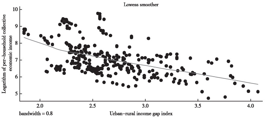
Lawess Smoother of Per-Household Collective Economic Income and Urban-Rural Income Gap Index (2010–2019)
Source: China Rural Business Management Statistics Annual Report (2011–2018), China Rural Policy and Reform Statistics Annual Report 2019, China Rural Cooperative Economy Statistics Annual Report 2019, China Statistics Yearbook (2011–2020).

Lawess Smoother of Per-Household Collective Economic Income and Per Capita Disposable Income of Rural Residents (2010–2019)
Sources: China Rural Business Management Statistics Annual Report (2011–2018), China Rural Policy and Reform Statistics Annual Report 2019, China Rural Cooperative Economy Statistics Annual Report 2019, China Statistics Yearbook (2011–2020).
2 Overview of China’s Rural Collective Economic Development: Sustained Growth and Spatial Differentiation
This paper first describes the growth of rural collective economic income in 2009– 2018 and then growth characteristics and geographic distribution differences of annual collective economic income from the respect of time and space with per-household collective economic income are aralyzed. Afterwards, the paper studies the distribution characteristics and growth trend of collective economic income in the eastern, central, western and northeastern region.[1]
2.1 China’s Rural Collective Economic Income Growth in 2009–2018
The total collective economic income measures the general scale of collective economic development, and per-household collective economic income is the total collective economic income divided by the total number of households. Because of different household numbers in each province, per-household collective economic income can measure the collective economic development in different regions more objectively. Figure 3 shows the developments of total collective economic income (national average) and per-household collective economic income (national average) of 30 provinces (autonomous regions or municipalities)[2] in China from 2009 to 2018. Both grew evidently, with the former growing by 79.73% and the latter 81.18% in a decade. That is, China’s collective economy operates at a good state, as the overall scale and average level of the collective economy continue to grow, and the collective economic benefits are enlarging on a yearly basis.

Developments of Total Collective Economic Income and Per-Household Collective Economic Income in Rural China (2009–2018)
2.2 Spatial Distribution of China’s Rural Collective Economic Income (Mean) in 2009–2018
Regional disparities are observed by averaging the per-household collective economic income of each province (autonomous region or municipality) in 2009– 2018. Generally, the per-household collective economic income was “high in the east and low in the west”. Specifically, Beijing, Tianjin, Shandong, Zhejiang, Jiangsu and Guangdong have the highest per-household collective economic income, and Inner Mongolia, Gansu, Qinghai, Sichuan, Chongqing, Guizhou, Guangxi and Anhui registered the lowest. It reveals that collective economic development is closely related with factors such as regional economic foundation, market resources and location.
2.3 Regional Growth of Per-Household Collective Economic Income in 2009–2018
According to the criteria for geographical division published by the National Bureau of Statistics (NBS) in 2005, 30 provinces (autonomous regions or municipalities) in China can be classified into the eastern, the central, the western and the northeastern region respectively. The eastern region covers Beijing, Tianjin, Hebei, Shanghai, Jiangsu, Zhejiang, Fujian, Shandong, Guangdong and Hainan. The central region covers Shanxi, Anhui, Jiangxi, Henan, Hubei and Hunan. The western region covers Chongqing, Sichuan, Guizhou, Yunnan, Shaanxi, Gansu, Qinghai, Ningxia, Xinjiang, Inner Mongolia and Guangxi. The northeastern region has Liaoning, Jilin and Heilongjiang. As shown in Table 1, the western and eastern regions have the most provinces (autonomous regions or municipalities), 36.67% and 33.33% respectively, and 20% and 10% in the central and the northeastern respectively.
Mean, Relative Mean and 10-Year Regional Growth Rate of Per-Household Collective Economic Income in China (2009–2018) Unit: yuan, %
| Region | Percentage of provinces (autonomous regions or municipalities) under jurisdiction | Year | Per-household collective economic income (mean) | Per-household collective economic income (relative mean) | Growth rate in 2009–2018 |
|---|---|---|---|---|---|
| 2009 | 3123.4523 | 2.2425 | |||
| Eastern region | 0.3333 | 81.95 | |||
| 2018 | 5683.2230 | 2.2522 | |||
| 2009 | 759.4778 | 0.5453 | |||
| Central region | 0.2000 | 57.72% | |||
| 2018 | 1197.8773 | 0.4747 | |||
| 2009 | 381.8737 | 0.2742 | |||
| Western region | 0.3667 | 126.07% | |||
| 2018 | 863.2856 | 0.3421 | |||
| Northeastern region | 0.1000 | 2009 2018 |
597.4983 729.2555 |
0.4290 0.2890 |
22.05% |
The eastern region was much higher than other regions in respect of the mean and relative mean (regional/national average) of per-household collective economic income. In 2008, the mean of per-household collective economic income in the east was more than four times that of the central, more than eight times that of the west, and more than five times that of the northeast. As of 2018, the regional income gap in collective economy had not been narrowing. The relative mean of per-household collective economic income in the eastern region was 4.7, 6.6 and 7.6 times higher than that in the central, western and northeastern respectively.
From the growth rate of per-household collective economic income (mean), the collective economy in the western and eastern regions grew the fastest at 126.07% and 81.95% respectively, and the central region was at 57.72%, while the northeast region grew the slowest at 22.05%. By 2018, the per-household collective economic income (mean) of the western region had exceeded that of the northeast to catch up with that in the central region. It shows that despite a weak foundation for developing the collective economy, the western region is strong in momentum of development so that its collective economic income has grown rapidly.
Figure 4 shows developments of per-household collective economic income in the eastern, central, western and northeastern regions in 2009–2018. In general, over the past decade the per-household collective economic income was growing, but regional disparities were evident. Specifically, the east surged ahead in the collective economic income, whereas the northeast grew the slowest, even left behind by the west since 2015.

Regional Growth of Per-Household Collective Economic Income in 2009–2018
Figure 5 shows the four regions’ share of collective economic income in 2009 (left) and 2018 (right). The eastern region’s share of collective economic income was as high as 75% in 2009. As of 2018, regional disparities in collective economic income had not been reduced, where the share of the eastern region remained the same, those of the northeastern and central regions further decreased, and that in the western region enlarged.

Four Regions’ Share of Collective Economic Income in 2009 (Left) and 2018 (Right)
With a study on China’s rural collective economic development it is concluded: a. China’s rural collective economy grows relatively rapidly, with the total collective economic income and per-household collective economic income increasing on a yearly basis. b. Regional disparities in collective economic income in rural China are serious. The eastern region takes a large lead in driving the collective economy, the western has grown its collective economic income the fastest with a good development momentum, and the central and northeastern regions have developed weakly.
3 Measuring the Regional Disparity of Rural Collective Economic Income in China
To accurately understand regional disparity of rural collective economic income in China, the Gini coefficient, Theil index, Atkinson index and other empirical approaches are applied to measure the sizes, types, and trends and characteristics of the disparity of per-household collective economic income in the four regions and nationwide in 2009–2018.
3.1 Approaches for Measuring Collective Economic Income Gap
This paper measures and decomposes regional disparity in per-household collective economic income in rural China with Gini coefficient, Theil index and Atkinson index, and reveals the size and source of regional disparity.
3.1.1 Gini Coefficient
Gini coefficient is the most common measure of income gap, and the calculation formula is:
where n is the total number of provinces (30), INCi is the per-household collective economic income of the i-th province, and E(INC) is the mean of per-household collective economic income of all provinces.
3.1.2 Theil Index
Theil index is another common indicator measuring regional income gap. Compared with Gini coefficient, it has two improvements. First, Gini coefficient is particularly sensitive to changes in the median value and fails to respond significantly to changes in the high- and low-income level, but Theil index has no such problems. Second, Theil index decomposes disparity into intra-group and inter-group types, making clearer the source of disparity.
First of all, China has four parts: the eastern, central, western and northeastern regions, according to NBS classification. Secondly, the Theil index that measures collective economic income is further divided into inter-group (different regions) and intra-group (different provinces in the same region) disparities in the form of:
TI represents Theil index of the overall disparity of per-household collective economic income in China, which can be divided into intra-group (different provinces in the same region) and inter-group (different regions) disparities. TW is intra-group
Theil index which measures the per-household collective economic income gap of different provinces in the same region; TB is inter-group Theil index that measures the per-household collective economic income gap among regions. In the formulas n is the total number of provinces (30), m is the number of regions (4), and nk represents the number of provinces included in the k-th region; INCi is per-household collective economic income of the i-th province, E(INC) is the mean of per-household collective economic income of all provinces, and E(INC)k is the mean of per-household collective economic income of the k-th region.
3.1.3 Atkinson Index
Theil index is derived from the entropy method in physics, while Atkinson index is from welfare economics. Therefore, Atkinson index has obvious social welfare implications in measuring the unequal distribution of income.
Atkinson index first calculates an equivalent sensitive equal income ye (defined as the total social welfare when everyone enjoys such an equivalent sensitive income). ye is calculated with the following formula:
When ye is defined, Atkinson index is expressed as:
In the formula, u is the mean and ye is the equivalent sensitive income (average). The more equitable the social income distribution is, the closer ye is to u, the smaller Atkinson index is. In calculating ye, INCi represents per-household collective economic income in different provinces; f (INCi) is the density function of the proportion of per-household collective economic income in different provinces; e is a self-selected index which reveals social acceptance of disparity, i.e., the relative sensitivity of income when it is transferred at different levels, and the range is from 0 to positive infinity. With the increase of e, the society expands the weight of transferring from the low-income level to the middle. Generally speaking, the common values of e are 0.5, 1 and 2, and 1 is selected for this paper.
Like Theil index, Atkinson index can be decomposed into intra-group and intergroup disparities, but with residuals, the sum of two parts after decomposition is not exactly equal to the Atkinson index.
3.2 Measurement Results
3.2.1 China’s Rural Collective Economic Income Gap Slightly Narrowed in 2009– 2018
As shown in Figure 6, the rural collective economic income gap changed not significantly in 2009–2018, with a slight decline. The downward trend of Gini coefficient and Atkinson index was evident, but Theil index even had a slight growth in 2011–2016. The reason may be that Theil index is most sensitive to changes of extreme values.

Measure of China’s Per-Household Collective Economic Income Gap in 2009–2018
Generally, China’s rural collective economic income gap has been narrowed by a small margin, and regional imbalances of collective economic income in a decade were not well solved.
3.2.2 Collective Economic Income Gap in Central and Western Regions Fell Remarkably in 2009–2018
(1) Gini coefficient. As shown in Figure 7, the Gini coefficient fell remarkably and the regional inter-provincial income gap gradually decreased in central and western regions in 2009–2018. The income gap among three northeastern provinces was small and the Gini coefficient fell slightly. However, the eastern region’s income gap was large and has not been significantly improved for a long term.

Changes in Gini Coefficient of Collective Economy in Different Regions of China in 2009–2018
(2) Theil index. As shown in Figure 8, the Theil index declined largely in the central and western regions in 2009–2018, representing a gradual narrowing in the inter-provincial income gap. The Theil index of the northeastern region is very small, with little obvious income gap. However, the eastern region is rather imbalanced in development, with a slight increase in Theil index.

Changes in Theil Index of Collective Economy in Different Regions of China in 2009–2018
(3) Atkinson index. As shown in Figure 9, Atkinson index is similar to Theil index in the results. In 2009–2018, the inter-provincial income gap in central and western regions gradually decreased. Three northeastern provinces had little obvious differences. However, the eastern region faced imbalanced growth—large inter-provincial disparities in collective economic income have been evident.

Changes in Atkinson Index of Per-Household Collective Economy in Different Regions of China in 2009–2018
3.2.3 China’s Inter-Region (Different Regions) Disparities in Collective Economic Income Were Large in 2009–2018
As shown in Table 2 and 3, the intra-group inequality and inter-group inequality after the decomposition by Theil index and Atkinson index are marked. It indicates that rural China has both intra-group (different provinces in the same region) and inter-group (different regions) inequalities in collective economic income, with the latter larger than the former, at more than 50% of the total. It means that spatial and geographical factors have great influence on the collective economic development.
Theil Index Decomposition of Per-Household Collective Economic Income Gap in 2009–2018
| Year | Total disparities | Intra-group disparities | Inter-group disparities | ||
|---|---|---|---|---|---|
| Disparity | Contribution (%) | Disparity | Contribution (%) | ||
| 2009 | 0.6394 | 0.2682 | 41.95 | 0.3712 | 58.05 |
| 2010 | 0.6175 | 0.2607 | 42.22 | 0.3568 | 57.78 |
| 2011 | 0.5797 | 0.2297 | 39.62 | 0.3440 | 59.34 |
| 2012 | 0.5915 | 0.2405 | 40.66 | 0.3510 | 59.34 |
| 2013 | 0.5946 | 0.2411 | 40.55 | 0.3534 | 59.43 |
| 2014 | 0.6036 | 0.2411 | 39.94 | 0.3626 | 60.07 |
| 2015 | 0.6090 | 0.2441 | 40.08 | 0.3649 | 59.92 |
| 2016 | 0.6355 | 0.2559 | 40.27% | 0.3796 | 59.73% |
| 2017 | 0.6304 | 0.2586 | 41.02% | 0.3719 | 58.99% |
| 2018 | 0.6220 | 0.2537 | 40.79% | 0.3683 | 59.21% |
Atkinson Index Decomposition of Per-Household Collective Economic Income Gap in 2009–2018
| Year | Total disparities | Intra-group disparities | Inter-group disparities |
|---|---|---|---|
| 2009 | 0.4726 | 0.2480 | 0.2987 |
| 2010 | 0.4512 | 0.2493 | 0.2689 |
| 2011 | 0.4361 | 0.2118 | 0.2845 |
| 2012 | 0.4258 | 0.2164 | 0.2672 |
| 2013 | 0.4238 | 0.2164 | 0.2646 |
| 2014 | 0.4264 | 0.2169 | 0.2676 |
| 2015 | 0.4264 | 0.2208 | 0.2639 |
| 2016 | 0.4347 | 0.2341 | 0.2620 |
| 2017 | 0.4290 | 0.2324 | 0.2561 |
| 2018 | 0.4248 | 0.2287 | 0.2542 |
After the four regions’ income gap of collective economy is measured, it is concluded: a. China’s rural collective economic income gap is evident with a featured imbalance, and has not been largely reduced for as long as a decade. b. From the income gap of different regions, while the eastern region far exceeded others in the collective economic income, it had an income gap that was marked and widened over the decade. The collective economic income gap in the northeast region is small, and that in the central and western regions has been narrowing. c. As for the source of disparities, more than 50% belongs to inter-group disparities (caused by different regions), which indicates the crucial impact of geographical location on collective economic income.
4 Spatial Convergence Analysis of China’s Rural Collective Economy
In this section, the spatial convergence model is applied to find out the changes in rural collective economic income, the impact of spatial location on collective economic income, and characteristics of β convergence and “club convergence” of rural collective economic income.
4.1 Data and Variables Selected for Spatial Convergence of Collective Economic Income
This paper uses panel data of 30 provinces (autonomous regions or municipalities) in the China’s Rural Business Management Statistical Annual Report 2009–2018 to study the spatial convergence of collective economic income. Definitions and descriptive statistics of the selected variables are shown in Table 4.
Introduction, Definition and Descriptive Statistics of Selected Variables
| Variable type | Variable dimension | Variable name | Variable definition | Mean | Standard deviation | |
|---|---|---|---|---|---|---|
| Dependent variable | Collective economic income growth | growth Logarithmic rate of per-household collective economic income | 0.0757 | 0.1314 | ||
| Core explanatory variable | Collective economic income | ln (INCi t , ) | Logarithm of per-household collective economic income | 6.941 | 1.0057 | |
| Control variable | Capital accumulation | ln K | Logarithm of per-household collective assets | 8.5705 | 1.3277 | |
| Technical progress | Information computerization | Aomputerized | Proportion of villages information with computerization | 0.5647 | 0.3231 | |
| Financial disclosure | Disclosure | Proportion of villages with financial disclosure | 0.9576 | 0.0670 | ||
| Government integrity | Administration | Proportion of violation amount of money of collective economic organizations to audited amount (negative indicator) | 0.0055 | 0.0608 | ||
4.2 Spatial β Convergence Analysis of Collective Economic Income
4.2.1 β Convergence: Definition and Model Introduction
According to Barro and Sala-i-Martin (1992), the β convergence of collective economic income means a province initially with low collective economic income has higher growth rate than that initially with high collective economic income. After a period of time, provinces with backward collective economy will catch up with leading provinces, and their collective economic income will converge to the same steady state.
β convergence is divided into absolute β convergence and conditional β convergence. Absolute β convergence is unconditional and can be reached without controlling any factors. Conditional β convergence holds that convergence depends on development-involved conditions, and only when factors, such as capital accumulation and technological progress, which influence collective economic growth, are controlled, there be will convergence.
During convergence, the collective economic development of geographically adjacent provinces may influence each other. Therefore, spatial factors are included in the analysis framework and a convergence model containing spatial factors is constructed. The form of spatial β absolute convergence model is as follows:
ln (INCi,t+1/INCi,t) represents the growth rate of per-household collective economic income in the i-th province during the t-period. ρWln (INCi,t+1/INCi,t) is the spatial lag term of the growth rate of explained variables, and ρ is the estimated coefficient, which indicates that the growth rate is spatially dependent when it is not 0. λWui,t is the spatial lag term of the perturbation term, of which λ is the estimated coefficient, indicating the perturbation term is spatially dependent when it is not 0. W is the spatial weight matrix. It is noted that ρ and λ are keys to distinguishing the spatial panel model from general panels, specifically:
When ρ≠0 and λ≠0, it is a spatial autocorrelation model (SAC).
When ρ≠0 and λ = 0, it is a spatial autoregressive model (SAR).
When ρ = 0 and λ≠0, it is a spatial error model (SEM).
The final applicable spatial model is identified by the spatial dependence test results of the dependent variable growth rate and the perturbation term in the empirical process.
β is the parameter to be estimated. If β<0 and the coefficient is significant, the collective economic income converges, otherwise it diverges. When convergence is reached, the rate of convergence ω and the period of convergence τ can be calculated with the formula:
The per capita output (Y/L) growth in Solow model results from per capita capital stock and technological progress and only technological progress will permanently increase per capita output. In absolute β convergence model, capital and technology factors influencing collective economic income are added to construct a spatial β conditional convergence model, the specific form of which is as follows:
lnK and As in (9) are control variables added, where lnK is capital accumulation, represented by the logarithm of per-household collective assets. As is technological progress, represented by villages with information computerization, financial disclosure openness and government integrity. Meanings and descriptive statistics of indicators are shown in Table 4.
4.2.2 β Convergence: Spatial Regression Results
The spatial β absolute convergence and conditional β convergence of collective economic income are tested. Firstly, Moran’s I reveals the applicability of the spatial model. In 2009–2018, the spatial correlation Moran’s I of per-household collective economic income of 30 provinces (autonomous regions or municipalities) is 0.216 and passes the significance test. There is a global positive correlation, indicating that the spatial econometric analysis is reasonable to use. Secondly, Hausman test significantly rejected the original assumption that there was no individual fixed effect, indicating the spatial fixed effect model was applicable. In choosing the specific forms of spatial model, three models are regressed. As shown in Table 5 and Table 6, the SAC is the most applicable—the explained variable and error item are spatially dependent.
Spatial β Absolute Convergence Regression Results of Rural Collective Economic Income in China
| SAC | SAR | SEM | |
|---|---|---|---|
| Convergence coefficient | −0.2438*** | −0.1849*** | −0.2015*** |
| β | (0.0388) | (0.0288) | (0.0328) |
| Spatial lag coefficient ρ(rho) | −0.3040** (0.1461) |
0.0140 (0.0896) |
— |
| Lag coefficient of error term λ (lambda) | 0.3639*** (0.1211) |
— | 0.1382* (0.0857) |
| Variance of error term | 0.0134*** | 0.0128*** | 0.0126*** |
| σ2 | (0.0011) | (0.0011) | (0.0011) |
| Maximum Log-likelihood l | 208.6191 | 205.6838 | 206.6961 |
| Rate of convergence ω | 3.105% | 2.272% | 2.500% |
| Period of convergence τ | 22 | 30 | 28 |
Note: ***, **, and * are significant at the statistical levels of 1%, 5%, and 10%, respectively.
Spatial β Conditional Convergence Regression Results of Rural Collective Economic Income in China
| SAC | SAR | SEM | |
|---|---|---|---|
| Convergence coefficient | −0.2678*** | −0.2316*** | −0.2458*** |
| β | (0.0388) | (0.0347) | (0.0368) |
| Capital accumulation | 0.0311* | 0.0254* | 0.0282* |
| lnK | (0.1873) | (0.0154) | (0.0172) |
| Information computerization | 0.0752* | 0.1125* | 0.1082* |
| Aomputerized | (0.0387) | (0.0703) | (0.0694) |
| Financial disclosure | 0.2730* | 0.2970 | 0.2998 |
| Disclosure | (0.1671) | (0.2744) | (0.2717) |
| Government integrity (Negative Indicator) Administration | −0.0748 (0.1266) |
−0.0880 (0.1295) |
−0.0858 (0.1288) |
| Spatial lag coefficient ρ (rho) | −0.2355* (0.1504) |
0.0417 (0.0896) |
— |
| Lag coefficient of error term λ (lambda) | 0.3134** (0.1345) |
— | 0.1354* (0.0792) |
| Variance of error term | 0.0134*** | 0.0124*** | 0.0124*** |
| σ2 | (0.0011) | (0.0011) | (0.0011) |
| Maximum Log-likelihood l | 210.9464 | 208.9820 | 209.9162 |
| Rate of convergence ω | 3.463% | 2.927% | 3.134% |
| Period of convergence τ | 20 | 24 | 22 |
Note: ***,**, and * are significant at the statistical levels of 1%, 5%, and 10%, respectively.
Firstly, observing the absolute convergence regression results in Table 5, three models all show that there is absolute spatial convergence in the growth of rural collective economic income. The convergence coefficient β is significantly negative in three models, revealing that every province has absolute β convergence in the collective economic income growth. Provinces with low collective economic income will catch up with leading provinces with the passage of time. Secondly, SAC shows the fastest rate of convergence, with 22 years for backward provinces catching up with leading provinces, followed by SEM, and SAR shows it takes 30 years to achieve convergence. To such point, provinces with backward collective economic income in rural areas still need a long time of effort and development to surpass leading provinces.
As shown as the conditional convergence regression results in Table 6, three models all reveal the spatial conditional convergence in China’s collective economic income growth. As factors such as capital accumulation and technological progress are controlled, the convergence coefficient β in the first row of Table 6 is significantly negative in three models, indicating the conditional β convergence exists in the growth of collective economic income in all provinces of China. Besides, the rate of conditional convergence is evidently faster than that of absolute convergence. When the capital and technical factors related to economic development are controlled, inter-provincial collective economy can present a faster convergance rate and a largely shortened period of convergence. When conditions influencing the collective economic income growth are controlled, three models are more similar in convergence results—the fastest is 20 years and the slowest is 24 years. Finally, capital accumulation, information computerization and financial diclosure produce relatively significant positive impact on the collective economic income growth. Violations (negative indicator) in the government integrity show a negative impact in three models, though they are insignificant. Generally, the growth of collective economic income is influenced by capital accumulation and technological progress. When these factors are controlled, the collective economy will converge faster.
4.3 Spatial Club Convergence Analysis of Collective Economic Income
Baumol (1986) put forward the theory of club convergence based on β convergence. Countries are divided into three types according to their income: rich, middle and poor, and are studied on the convergence of income levels. The results show that the convergence rate of rich countries is the fastest, and that of middle-income countries is much weaker, while that of poor countries is not significant. It is believed areas of higher economic development level are stronger in technology and diffusion capabilities. The theoretical implication of club convergence is that countries or regions with similar economic foundation will converge to the same local stable state. Therefore, based on their initial conditions, different regions will form different clubs in development and regions with similar conditions within the same club will converge in development.
On studying the club convergence of collective economic income, 30 provinces (autonomous regions or municipalities) are divided into three clubs according to three criteria—geographical location, economic development and spatial cluster. Then existence of club convergence is verified respectively.
4.3.1 Geographical Club Division and Spatial Convergence Model
Based on geographical locations, 30 provinces (autonomous regions or municipalities) are divided into the eastern, central, western and northeastern clubs. Clubs and their respective provinces are shown in Table 7. Assuming that the initial conditions of collective economic development in the four clubs are different, the collective economic development of provinces with similar internal conditions in a club will reach convergence.
Geographical Club Division and Provinces in Each Club
| Geographic club | Eastern region | Central region | Western region | Northeastern region |
|---|---|---|---|---|
| Provinces (autonomous regions or municipalities) | Beijing, Tianjin, Shanghai, Shandong, Guangdong, Jiangsu, Hebei, Zhejiang, Hainan, Fujian | Anhui, Shanxi, Jiangxi, Henan, Hubei, Hunan | Yunnan, Inner Mongolia, Sichuan, Ningxia, Guangxi, Xinjiang, Gansu, Guizhou, Chongqing, Shaanxi, Qinghai | Heilongjiang, Jilin, Liaoning |
Table 8 reports the SAC regression results for the geographical club. Firstly, the spatial lag term coefficient and the spatial error term coefficient are of poor significance, because the spatial model mainly relies on geographical differences to introduce spatial factors for regression. After all provinces are geographically divided into clubs, spatial locations of the provinces in each club are similar, which means eliminating the spatial differences. Therefore, the coefficients of spatial lag term and spatial error term are no longer significant, and the convergence coefficient and regression results of control variables are basically similar to the panel fixed effect regression.
Spatial Regression Results of Geographical Club Convergence for Rural Collective Economic Income in China
| Eastern region | Central region | Western region | Northeastern region | |
|---|---|---|---|---|
| Convergence coefficient | −0.3059*** | −0.2621*** | −0.2860*** | −0.5852*** |
| β | (0.0683) | (0.0779) | (0.0707) | (0.1478) |
| Capital accumulation | 0.0652* | 0.0205 | 0.0180 | 0.0532 |
| lnK | (0.0390) | (0.0340) | (0.0172) | (0.0474) |
| Information computerization | 0.2172 | 0.3109* | 0.2483* | 0.4401** |
| Aomputerized | (0.2113) | (0.1720) | (0.1515) | (0.2073) |
| Financial disclosure | 1.0306 | 1.2450 | 1.0293** | 9.6925 |
| Disclosure | (0.6059) | (1.2819) | (0.4270) | (7.2635) |
| Government integrity (negative indicator) Administration | 0.1674 (0.1688) |
−3.4294 (4.5450) |
4.2241 (6.3150) |
−21.2199* (12.2309) |
| Spatial lag coefficient | −0.0291 | 0.2574 | 0.1158 | −0.2409 |
| ρ(rho) | (0.1579) | (0.2317) | (0.3471) | (0.2497) |
| Lag coefficient of error term | 0.1743 | 0.1357 | −0.1477* | −0.0462 |
| λ (lambda) | (0.1548) | (0.3029) | (0.3877) | (0.3289) |
| Variance of error term | 0.0130*** | 0.0085*** | 0.0163*** | 0.0048*** |
| σ2 | (0.0018) | (0.0015) | (0.0022) | (0.0012) |
| Maximum Log-likelihood l | 72.3351 | 53.6218 | 68.7870 | 34.8861 |
| Rate of convergence ω | 4.057% | 3.377% | 3.734% | 9.777% |
| Period of convergence τ | 17 | 21 | 19 | 7 |
| obs | 90 | 54 | 99 | 27 |
Note: ***, **, and * are significant at the statistical levels of 1%, 5%, and 10%, respectively.
Secondly, the convergence coefficient β is significantly negative in four clubs, which means that the collective economic income has converged in different geographical clubs. Further, the rate of convergence is the fastest and the period is the shortest in the northeast region. The equilibrium is quickly reached because the differences in three northeastern provinces’ collective economic development are small. The rate of convergence in the eastern and western regions is moderate. It is predicted that the convergence may be achieved in 17 and 19 years. The central region registers the slowest rate and it may take 21 years to achieve convergence. The results are in line with the previous section in the measurement results of regional growth and disparities of collective economic income. As northeastern provinces have light income disparities, the eastern region has a high-level collective economic income development, and the western takes on a strong growth momentum for collective economic income, they can reach convergence faster than the central region.
Finally, capital accumulation, a control variable, is crucial to the eastern region, while technical indicators like information computerization are significant in the central, western and northeastern regions. It reveals the development of collective economic income in the eastern region has been ertered the stage of capital operation to a great extent, while the central, western and northeastern regions, which are relatively underdeveloped, need support from technological progress such as information infrastructure.
4.3.2 Economic Club Division and Spatial Convergence Model
Club convergence was first proposed based on the economic level. Then 30 provinces (autonomous regions or municipalities) are divided into the developed, developing and underdeveloped clubs, according to their collective economic development (per-household collective economic income), as shown in Table 9. Assuming that the initial conditions of the three clubs are different, the collective economic development of provinces with similar conditions in each club will converge.
Economic Club Division and Provinces in Each Club
| Economic clubs | Developed | Developing | Underdeveloped |
|---|---|---|---|
| Provinces (autonomous regions or municipalities) | Beijing, Tianjin, Shanghai, Shandong, Shanxi, Guangdong, Jiangsu, Zhejiang, Hainan, Hubei | Jilin, Yunnan, Xinjiang, Jiangxi, Hebei, Henan, Hunan, Fujian, Liaoning, Shaanxi | Inner Mongolia, Sichuan, Ningxia, Anhui, Guangxi, Gansu, Guizhou, Chongqing, Qinghai, Heilongjiang |
Table 10 reports the SAC regression results of three economic clubs. Firstly, the spatial lag term coefficient and spatial error term coefficient of developed and developing clubs are significant and those of the underdeveloped club are not. It may be that in underdeveloped club, geographical locations are similar and are no longer important for collective economic development. The differential locations in developed and developing regions present evident impact.
Spatial Regression Results of Economic Club Convergence for Rural Collective Economic Income in China
| Underdeveloped | Developing | Developed | |
|---|---|---|---|
| Convergence coefficient | −0.2353*** | −0.3020*** | −0.3786*** |
| β | (0.0663) | (0.0687) | (0.0685) |
| Capital accumulation | 0.0035 | 0.0327* | 0.0539* |
| lnK | (0.0267) | (0.0207) | (0.0341) |
| Information computerization | 0.1040* | 0.0579 | 0.1379 |
| Aomputerized | (0.0617) | (0.1557) | (0.1830) |
| Financial disclosure | 0.7785* | −0.4888 | 1.5343** |
| Disdosure | (0.4201) | (0.8487) | (0.6443) |
| Government integrity (Negative Indicator) Administration | 0.9896 (6.7786) |
−2.5187 (4.6850) |
0.2888 (0.1790) |
| Spatial lag coefficient | 0.0211 | −0.4753*** | −0.0329* |
| ρ (rho) | (0.3146) | (0.1021) | (0.1753) |
| Lag coefficient of error term | −0.0551 | 0.5737*** | 0.2681* |
| λ (lambda) | (0.3294) | (0.0963) | (0.1573) |
| Variance of error term | 0.0173*** | 0.0085*** | 0.0138*** |
| σ2 | (0.0023) | (0.0015) | (0.0019) |
| Maximum Log-likelihood l | 60.2388 | 97.2240 | 69.5617 |
| Rate of convergence ω | 5.286% | 3.995% | 2.981% |
| Period of convergence τ | 23 | 17 | 13 |
| obs | 90 | 90 | 90 |
Note: ***, **, and * are significant at the statistical levels of 1%, 5%, and 10%, respectively.
Secondly, the convergence coefficient β is significantly negative in three clubs, which means that collective economic income has converged in different economic clubs. Further, the developed region shows the fastest rate and the shortest period of convergence, and the convergence is expected to reach within 13 year, followed by the developing region, with convergence to be achieved in 17 years. The underdeveloped region has the slowest convergence which can take 23 years to reach. It reveals that regions with higher levels of economic development have good foundation, high technological level and strong diffusion capacity.
Finally, the control variable, capital accumulation, is significant for the developed and developing regions, while the indicators, such as information computerization and financial disclosure, are more significant in the underdeveloped region. It means that developed and developing regions relies more on capital strength in growing their collective economic income, while the underdeveloped needs more support from technological progress.
4.3.3 Spatial Club Division and Spatial Convergence Model
Spatial clubs are divided by Moran’s I scatterplot drawn with per-household collective economic income (mean) in 2009–2018. The distribution is shown in Figure 10. The Moran’s I scatterplot divides 30 provinces (autonomous regions or municipalities) into clusters, including H-H (high-high), L-H (low-high), L-L (low-low) and H-L (high-low). Specifically, the H-H (high-high) cluster is in the first quadrant, where the provinces have a high level of development and so do the neighboring provinces. The L-H (low-high) cluster is in the second quadrant, where the development level of these provinces is low but that of the neighboring provinces is high. The L-L (low-low) cluster is in the third quadrant, where the development level of these provinces is low and so is that of the neighboring provinces. The H-L (high-low) cluster is in the fourth quadrant, where the development level of these provinces is high and that of the neighboring provinces is low. The Moran’s I value of collective economic development is greater than 0, with 22 provinces in H-H (high-high) and L-L (low-low) clusters, 73.33%. It means that the spatial spillover effect of collective economic development in China is relatively obvious, with spatial positive correlation in most provinces.

Moran’s I Scatterplot of Per-Household Collective Economic Income (Mean) of Each Province in 2008–2019
The 30 provinces (autonomous regions or municipalities) belong to four clubs, based on the spatial clusters divided by Moran’s I. Each club and its provinces are shown in Table 11. Assuming that the initial conditions of these clubs are different, the collective economic development of provinces with similar club internal conditions will converge.
Spatial Club Division and Provinces in Each Club
| Spatial clubs | H-H (high-high) | L-H (low-high) | L-L (low-low) | H-L (high-low) |
|---|---|---|---|---|
| Provinces (autonomous regions or municipalities) | Beijing, Tianjin, Shanghai, Zhejiang, Jiangsu | Hebei, Anhui, Jiangxi, Guangxi, Hainan, Fujian | Shanxi, Henan, Jilin, Liaoning, Heilongjiang, Hubei, Hunan, Inner Mongolia, Sichuan, Yunnan, Xinjiang, Guizhou, Chongqing, Shaanxi, Ningxia, Qinghai, Gansu | Shandong, Guangdong |
Table 12 reports the SAC regression results of spatial clubs. Firstly, the spatial lag coefficient and spatial error coefficient of H-H (high-high) and L-L (low-low) clubs are significant, while those of the L-H (low-high) club are insignificant, because the spatial spillover effect in spatially positively correlated areas is more obvious, while the H-L (high-low) club cannot report both coefficients as a result of the small number of samples.
Regression Results of Spatial Club Convergence for Rural Collective Economic Income in China
| H-H | L-H | L-L | H-L | |
|---|---|---|---|---|
| Convergence coefficient | −0.3061*** | −0.2801*** | −0.2892*** | −0.2567*** |
| β | (0.0728) | (0.0840) | (0.0539) | (0.0959) |
| capital accumulation | 0.0583* | 0.0395 | 0.0218 | 0.0262* |
| lnK | (0.0368) | (0.0458) | (0.0263) | (0.0139) |
| Information computerization | −0.0892 | 0.1791* | 0.0715 | 0.0521 |
| Aomputerized | (0.0639) | (0.1032) | (0.1173) | (0.0676) |
| Financial disslosure | 0.0186 | −0.2810 | 0.7096** | 0.0970 |
| Disclosure | (0.3023) | (0.6925) | (0.3706) | (0.3934) |
| Administrative Integrity (Negative Indicator) Administration | 0.0996 (0.6566) |
0.0330 (0.2088) |
−0.8939 (3.7410) |
−27.0886 (40.2704) |
| Spatial lag coefficient | −0.7464*** | −0.1505 | −0.3416* | —— |
| ρ (rho) | (0.0622) | (0.2703) | (0.2153) | |
| Lag coefficient of error term | 0.8158*** | 0.1716 | −0.3759* | —— |
| λ (lambda) | (0.0414) | (0.3046) | (0.2082) | |
| Variance of error term | 0.0006*** | 0.0251*** | 0.0128*** | 0.0007*** |
| σ2 | (0.0002) | (0.0043) | (0.0016) | (0.0002) |
| Maximum Log-likelihood l | 76.4741 | 25.8408 | 120.0310 | 40.5008 |
| Rate of convergence ω | 4.060% | 3.652% | 3.793% | 3.296% |
| Period of convergence τ | 17 | 19 | 18 | 21 |
| obs | 45 | 54 | 153 | 18 |
Note: ***, **, and * are significant at the statistical levels of 1%, 5%, and 10%, respectively.
Secondly, convergence coefficient β is significantly negative in four clubs, indicating that different economic clubs will achieve convergence. The rate of convergence is the fastest and the period is the shortest in the H-H (high-high) club, whose convergence is to reach in 17 years. The L-H (low-high) and L-L (low-low) clubs will converge in 19 years and 18 years respectively, while the H-L (high-low) club is the slowest and it will take 21 years to converge. In general, except for the H-L (high-low) club, which includes only two provinces, Shandong and Guangdong, with slow rate in convergence, the rate and period of convergence in other spatial clubs are not significantly different. It may mean that the spatial division based on Moran’s I enables different types of clubs to converge in a similar time period.
Finally, the control variable, capital accumulation, shows a significant impact in the H-H (high-high) and H-L (high-low) clubs, while information computerization is significant in the L-H (low-high) club and financial disclosure in the L-L (low-low) club. It may reveal that clubs of high-level development rely more on capital strength, while those of low-level development need more support from technological progress.
5 Conclusions and Recommendations
The paper demonstrates the importance of rural collective economic organizations in growing farmers’ income and narrowing the relative urban-rural income gap. Based on the 2009–2018 data of rural collective economic development of 30 provinces (autonomous regions or municipalities), this paper describes and measures regional disparities and evolution of rural collective economic income in China, and with the spatial econometric model, summarizes typical facts of convergence in rural collective economic income, and explains primary influencing factors for different types of regional development.
The main findings as follows. a. Geographical location is the main factor influencing rural collective economic income in China. The growth of collective economic income in the eastern region surges ahead, and that in the western region is the fastest, while that in the central and northeastern regions is relatively weak. The income gap around eastern region is obvious. The collective economic income gap in the northeast region is relatively small. The income gap in the central and western regions has been narrowing. More than 50% of the disparities in China’s collective economic income come from inter-group differences in different geographical locations. b. Collective economic income has absolute convergence and conditional convergence. It will take 22–30 years for backward provinces to catch up with leading provinces. When technical indicators such as capital accumulation and information computerization are controlled, the rate of convergence is shortened to 20–24 years, i.e. there is conditional convergence, and capital accumulation, information computerization and financial disclosure have a relatively significant positive effect on the collective economic income growth, and government integrity shows a positive impact in three models. c. Spatial club convergence is evident. Four clubs are distinguished based on geographic locations, with convergence to be achieved in 17 and 19 years for the eastern and western regions, respectively, and 21 years for the central region. Capital accumulation influences significantly in the eastern region, and technical indicators such as information computerization are significant in the central, western and northeastern regions. Three clubs are distinguished by the development level, and the convergence is expected by 13 years in the developed region, 17 years in the developing region and 23 years in the underdeveloped region. The control variable, capital accumulation, is more significant for developed and developing regions, while indicators such as information computerization and financial disclosure are more significant in the underdeveloped region. Based on the spatial correlation, four clubs are distinguished, and the spatial spillover effect of collective economic income is relatively obvious and there is a spatial positive correlation in most provinces.
The collective economic income gap among regions must be reduced to drive the rural revitalization strategy for the balanced, coordinated development between urban and rural areas and among regions. a. A central structural guiding fund for collective economic development shall be set up. Support must be differential in the four regions, referred to Moran’s I, for the convergence of the income gap will reach within a similar time period. For spatially L-L provinces, financial investment must be stepped up to break the low-level equilibrium trap of spatial club convergence. b. Different ways of investing shall be applied for different regions. For the eastern region, strategies of “building a county with capital” and “building a town with capital” will be taken to activate the financial market and revonate old villages, factories and towns. For the western region, efforts will be to speed up constructing information infrastructure for collective economic organizations. c. The governance mechanism for rural collective economic and governance performance of collective economic organizations must be improved from the aspects of Party leadership, special corporation governance structure, community governance and administrative supervision.
References
Bai, Z., Wang, Q., & Lai, G. (1993). Analysis on Trends and Factors of Rural Residents’ Inter-Region Income Differences in China. Issues in Agricultural Economy (Nongye Jingji Wenti), 10, 30−35.Search in Google Scholar
Huang, Z., Wang, M., & Song, Y. (2005). Study of Income Gap of Rural Residents: An Analysis Framework Based on Micro-Perspective of Villages. Management World (Guanli Shijie), 3, 75−84.Search in Google Scholar
Sala-i-Martin, X. (1996). The Classical Approach to Convergence Analysis. Economic Journal, 106(437), 1019−1036.10.2307/2235375Search in Google Scholar
Shorrocks, A. (1984). Inequality Decomposition by Population Subgroup, Econometrica, 52(6), 1369−1386.10.2307/1913511Search in Google Scholar
Wei, H., (1996). China’s Rural Income Differences and the Decomposition. Economic Research Journal (Jingji Yanjiu), 11, 66−73.Search in Google Scholar
Wu, Z., & Song, H. (2007), Empirical Analysis of Gap in China’s Inter-Village Gross Social Product: Based on a Survey of 309 Villages in China. Management World (Guanli Shijie), 11, 54−62. See Rural Economy Center of Ministry of Agriculture (2008), Report on Rural China 2007. China Financial and Economic Publishing House. (in China)Search in Google Scholar
Zhang, P. (1992). Income Distribution Among Rural Residents in China. Economic Research Journal (Jingji Yanjiu), 2, 62−69.Search in Google Scholar
Zhang, P. (1998). Regional Income Inequality of Rural Residents and Non-Agricultural Employment in China. Economic Research Journal (Jingji Yanjiu), 8, 59−60.Search in Google Scholar
© 2022 Xueyuan Chen et al., published by De Gruyter
This work is licensed under the Creative Commons Attribution 4.0 International License.
Articles in the same Issue
- Frontmatter
- The Impacts of the Growth of the Three Industries and Industrial Price Structural Changes on China’s Economic Growth between 1952 and 2019
- Sub-Provincial Fiscal Expenditure Decentralization Structure: A Case in China
- Analysis on Regional Income Gap and Spatial Convergence in China’s Rural Collective Economy
- Nonlinear Shock Effect of China’s Fiscal Policy on Total Factor Productivity—Based on the Dual Perspective of Aggregate and Structure
- Does Internet Use Improve the Income of Residents? —Empirical Evidence from CGSS2017
- Promoting the Integration of China’s Tourism Industry into the New Development Pattern with Dual Circulation