
Impact of Technological Progress and Industrial Structure Distortion on Energy Intensity in China
-
Xiaobo Shen


Abstract
The paper measures the industrial structure distortion (ISD) index by region in China from 1978 to 2016 using data on employment and output shares of the three industries. It also analyzes the impact of ISDs by region on energy intensity using a spatial panel model. The results show that since the reform and opening up, the ISD index by region has declined significantly, with the lowest index in the eastern region, the medium one in the central region and the highest in the western region. The estimated results of the spatial econometric model indicate that there is a significant inter-regional dependence of energy intensity in China; there is a significant indirect effect of ISD, despite no significant direct effect on energy intensity; in terms of total effect, ISD is an important factor inhibiting the decline of energy intensity. The results also unveil that higher energy prices and foreign trade are positive factors declining energy intensity, while FDI worsens energy intensity and R&D spending has no significant positive impact on curbing energy intensity. In order to reduce energy intensity, China should work to eliminate the micro cause of ISDs, promote the transfer of agricultural labor, establish a market-oriented mechanism for energy price formation, and enhance the efficiency of R&D spending.
1 Introduction
Over the past 40 years of reform and opening up, China has seen its total energy consumption increase rapidly, but the total energy intensity (PTEI) and the energy intensity by industry have been declining in most years. During the same period, China has also witnessed significant changes in industrial structure, with the share of agricultural output declining markedly, that of the secondary industry dropping slowly and that of the tertiary industry rising steadily (see Figure 1). According to the literature examining changes in China’s energy intensity through decomposition analysis, the decline in China’s energy intensity is attributed primarily to that in energy intensity within each industry (i.e., technical effect), while structural changes make little or no contribution to the decline in China’s energy intensity (Liao et al., 2007; Ma and Stern, 2008; Wu, 2012; Tan and Lin, 2018). Regionally, the change in industrial structure makes a negative contribution to the descending energy intensity (Wu, 2012).
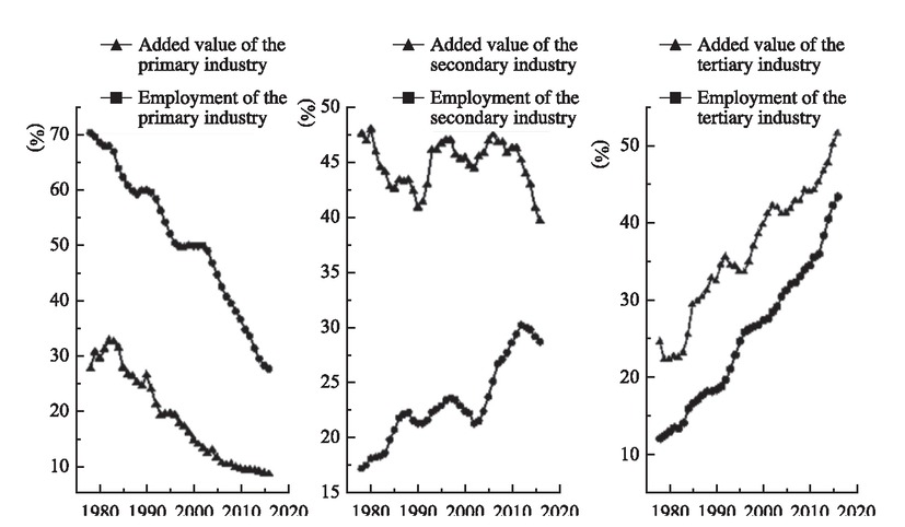
Shares of Added Value and Employment across Three Industries
The change of industrial structure means the intersectoral shift in output and employment share. Based on a frictionless general equilibrium model, Ando and Nassar (2017) demonstrated that labor productivity is equal across all sectors under the normal condition that labor may freely enter and exit the labor market. The equalization of sectoral labor productivity means that, for any sector, the shares of output and employment are also necessarily equal. The share of output in one sector of the economy deviates from its share of employment, signaling a reverse deviation in the other sectors. There are ISDs in relative equilibrium. Although the changes in the output and employment shares of China’s three major industrial sectors since the reform and opening up have been aligned with the general trend manifested by developed countries, evident gaps could be found between the output and employment shares by industry (see Figure 1). This implies that structural distortions are marked in the change of industrial structure in China. Such structural distortions inevitably have a negative impact on the allocation efficiency of resources (including energy), which may hinder the due reduction in energy intensity.
Based on the method by Ando and Nassar (2017), the paper aims to measure the trends of ISDs in China over the past 40 years by region and assess the impact of ISDs on energy intensity using a spatial econometric model. The contribution of this paper covers the following two aspects. First, we analyze the impact of exogenous technological progress on changes of industrial structure based on the model of Nunn and Qian (2011). Second, unlike the existing literature for studying the impact of industrial structure changes on energy efficiency, this paper is meant to analyze the impact of distorted industrial structure on energy intensity. The outcome demonstrates that distorted industrial structure is generally an important factor affecting energy intensity in China.
The paper is composed of the following parts. Section 2 explores theoretically the impact of exogenous technological progress on inter-sectoral shifts of output and employment shares based on the model of Nunn and Qian (2011). Section 3 presents Ando and Nassar (2017) approach to measuring ISDs based on the deviation of industry shares from employment shares. Section 4 discusses the model setup, variable selection and data. Section 5 estimates the impact of ISDs on energy intensity in China using a spatial econometric model. Section 6 summarizes the conclusions and makes policy recommendations.
2 Technological Progress and Industrial Structure Changes
Although no general economic theory exists to date to explain structural changes, productivity improvement stemming from innovation and technological change is perceived as one of the main drivers of structural changes. For example, Kuznets (1971) argued that rapid changes in the structure of production are inevitable given different effects of technological innovation on production sectors. Nunn and Qian (2011) proposed a simple two-sector model to examine the impact of labor productivity improvement from exogenous technological progress in the agricultural sector on population size and urbanization. We note that the model can be used to examine the impact of technological progress on industrial structural changes. The paper would explain how technological progress affects the industrial structure through the model.
We suppose an economy consisting of agriculture and manufacturing sectors, with individuals opting to work in one of them. LF and LW represent the number of farmers engaged in the agricultural sector and that of workers employed in the manufacturing sector, respectively. The total workforce is normalized to 1. Each worker in the manufacturing sector always makes one unit of manufactured goods, while each farmer generally produces e unit of agricultural products. It is assumed that the preferences of workers and farmers for two commodities are the same, and they are determined by the utility function
If the price of manufactured goods is normalized to 1, then the price of agricultural products is p.
Farmers maximize utility subject to their budget constraints, that is:
The constraint is expressed as
Similarly, the problem of maximizing the utility of manufacturing workers is expressed as:
The constraint is denoted as
From the first-order conditions of the maximization problem of farmers and workers, we can get:
The free flow of factors and the clearing of labor market require no difference between individuals working in the two sectors, i.e., the labor productivity of the two sectors is equal, thus pe = 1.
Requirements for clearing the agricultural product market are expressed as follows:
We take equation (3) into (4) and use pe = 1, obtain labor forces (also the labor share) of the agricultural sector in equilibrium.
Correspondingly, the labor of the manufacturing sector (also the labor share) in equilibrium is denoted as:
The revenue of agricultural sector is equivalent to its workforce multiplied by the labor productivity and then by the price of agricultural products, that is:
Similarly, the total revenue of the manufacturing sector is expressed as:
Thus, the total revenue of the economy can be denoted as:
The revenue share of the agricultural sector is expressed as:
Correspondingly, the revenue share of the manufacturing sector is denoted as:
It can be seen from equations (5) and (10) that, in equilibrium, the labor and revenue shares of the agricultural sector are equal; similarly, equations (6) and (11) indicate that the shares of labor and output in the manufacturing sector are equal in equilibrium. Therefore, an important conclusion of the above model is that, for an economy with a free flow of labor, the share of employment in any sector is always equal to that of revenue in equilibrium. The conclusion is consistent with that reached by Ando and Nassar (2017).
In the following, we examine how exogenous technological progress affects changes in industrial structure based on the above model. First, we assume that exogenous technological progress in the agricultural sector results in an increase in the labor productivity of agricultural sector. What is the impact of productivity gains resulting from exogenous technological progress on employment and output shares of the sector? We find the derivative of equation (5) with respect to productivity e as follows:
Obviously,
According to Nunn and Qian (2011), σ was used to measure the inverse
Second, what is the outcome if there is exogenous technological progress in the manufacturing sector? After the increased labor productivity in manufacturing, maintaining the conditions of labor market clearing in both sectors is required to either enhance the agricultural labor productivity e by the same margin or increase agricultural prices p by the same amount. In the absence of technological progress in the agricultural sector, transferring agricultural labor to the industrial sector is the only way to increase agricultural productivity or the price of agricultural products. Such an approach can lead to an equal decline in the share of employment and output in the agricultural sector and a correspondingly equal increase in the share of employment and revenue in the manufacturing sector. As a result, although employment and output, after technological progress in manufacturing, may shift between sectors, the share of employment in any sector is still equal to that of revenue.
Finally, if technological progress can be made in both sectors simultaneously. In this case, either the rate of technological progress is the same in both sectors, or the rate is relatively faster in any sector. In either case, it can still prove that the share of employment and revenue in either sector remain ultimately the same. Combining the three above scenarios, it is known that, under conditions of free labor mobility, technological progress leads to changes in the industrial structure and inter-sectoral shifts in the shares of output and employment, but the shares of employment and output remain equal in any sector. The finding provides a theoretical basis for measuring distortions in industrial structure and identifying the effects of structural distortions and technological progress on energy intensity.
3 ISDs and Energy Intensity
3.1 ISDs and Their Measurements
The above theoretical models suggest that, in a market economy with free entry and exit of labors and perfect competition, the quest to maximize the interests of economic entities will ensure the efficient allocation of productive resources such as labor for various purposes, resulting in equal labor productivity across sectors. However, when the free flow of factors is impeded, intersectoral differences in labor productivity emerge arise, resulting in distortions and imperfections in the economy. So, how should we measure the distortion in the economy? According to the studies of Nunn and Qian (2011) and Ando and Nassar (2017), equilibrium, under a free flow of factors, requires that labor productivity be equal across sectors, with the result that the shares of output and employment are necessarily equal in any sector. Based on the finding, Ando and Nassar (2017) proposed a method to measure ISDs using the Euclidean distance between employment and output shares.
In supposing a country has N sectors, we let VAi and Li represent the added value and employment of sector i, respectively. The number of employed persons Li refers to the total one of employers, employees and self-employed persons in sector i. Ando and Nassar (2017) defined the Euclidean distance between added value and employment shares as:
di is the distance between shares of employment and output for sector i, and d is the Euclidean distance between shares of added value and employment in the economy as a whole. Obviously, if the distance d is equal to zero, it implies equalization of sectoral labor productivity:
Pi is the sector i’s labor productivity, while P is the labor productivity of the economy as a whole.
Under the condition that labor may freely enter and exit the labor market, people have an incentive to move from sectors with low labor productivity to those with high labor productivity, which can be expected as d→0, unless there is some barriers preventing the convergence of labor productivity. In this sense, d represents the overall distortion or ISD in an economy. The bigger d gets, the more distorted the economy turns. Also, di is used to measure the distortion of the sector i. di > 0 indicates that too many labor forces are involved in sector i, and vice versa.
In section 2, the findings of the theoretical analysis unveil {d,di}, an important property of the distortion index, meaning the index only reflects ISD due to market imperfections and policy distortions, and is not affected by technological progress. The results imply that the ISD index is exogenous to technological progress. It makes it possible for section 5 to identify the effects of ISD and technological progress (captured by R&D expenditure, FDI and foreign trade) on energy intensity.
3.2 Industrial Structure Distortion and Energy Intensity
Theoretically, any distortion leads to low-efficiency or zero-efficiency allocation of resources. In this sense, the distorted industrial structure necessarily increases energy intensity. The research of Nunn and Qian (2011) and Ando and Nassar (2017) demonstrated that the distorted industrial structure means the heterogeneity of sectoral labor productivity. In comparison to the equalization of labor productivity across sectors, labor is over-inputted relative to the size of its output in sectors with lower labor productivity, while it is under-inputted relative to the size of its output in sectors with higher labor productivity. This misallocation of labor resources at the industrial level essentially stems from that of resources at the micro level. The misallocation of micro-level resources often arises from distortions of product and factor markets. Product market distortions are commonly found in government regulations over energy prices. Currently, prices of energy products such as electricity and oil are strictly regulated by the Chinese government, while natural gas is priced under the guidance of the government. Energy prices do not adequately reflect the scarcity of energy and the externality of the environment. As a result, there is some price distortion of energy products in China (Hang and Tu, 2007; Ju et al., 2017). Evidently, the distortion must reduce the overall energy efficiency.
Distortions in factor markets affect the relative prices of labor and capital, which can lead to misallocation of resources. Take China’s restrictions on rural labor moving into cities and towns (such as hukou restrictions) as an example. This restriction keeps a large number of labor in the agricultural sector where labor productivity is already low. The surplus labor supply depresses the relative price of labor and capital. Farmers, governed by the cost minimization motive, would substitute labor for capital. In the agricultural sector, energy and capital (agricultural machinery) are usually complementary. The substitution of labor for capital also means the relative decline of energy utilization in agricultural production. The result is a relative decline in energy intensity of the agricultural sector. In the industrial sector, regulation of labor migration raises the relative price of labor. For a given output, a producer can substitute capital for labor in order to reduce the cost of production. In most cases, such practice would lead to an increase in energy use, thus enhancing energy intensity of the industrial sector. With a much higher share of output in the industrial sector than in the agricultural sector, the PTEI derived from a weighted average (the weight is sectoral output share) of energy intensity across sectors is bound to deteriorate. Such restrictions widen the gap in labor productivity between the agricultural sector and the industrial sector, compared to the situation where there is no regulation of rural labor migration. They reflect the fact that the share of labor in the agricultural sector is much higher than its share of output, while the opposite is true in the industrial sector, where the share of labor is lower than that of output. This is exactly what we mean by ISD. Thus, distortions in micro factor markets and ISDs are essentially two sides of the same coin, with the result that leads to resource misallocation and thus reduce the efficiency of resource allocation (including energy efficiency).
4 Empirical Models, Variables and Data
4.1 Model Setup
The above theoretical analysis suggests that ISD is an important factor affecting the PTEI. However, the ISD index in a region is measured based on the methodology in the previous section, with the premise that factors move only across industries within a region. In practice, however, factors flow between regions, in addition to between various industries within a region. Especially when there are significant differences in labor productivity and the resulted differences in wage between regions, the movement of labor factors across provinces and regions is more common and may even be more important than that between industries within regions. In this scenario, the ISDs in different regions may be intrinsically linked. In other words, the ISD in a region may affect those in other regions. The spatial correlation of distortions in industrial structure also means that economic output and energy use in different regions are also spatially correlated. As such, the energy intensity in a region is influenced not only by distortions in its own industrial structure, but also by those in industrial structures of other regions. To analyze the spatial correlation of ISDs and their impact on energy intensity, we set up several spatial econometric models as follows.
ln
The equation (15), commonly referred to as a spatial autoregressive model (SAR), was used to only consider the spatial correlation of explained variables. The equation (16), representing a spatial autocorrelation model (SAC), was utilized to consider the spatial correlation of explained variables and error terms. The equation (17), a spatial Durbin model (SDM), was applied to consider the spatial dependency of both the explained and explanatory variables.
4.2 Selection and Definition of Variables
The explained variable in this paper is the regional energy intensity, while the core explanatory variable the ISD index. The first control variable we choose is energy price. Energy price is one of the key driving forces for improving energy intensity. Many studies revealed significantly negative correlation coefficients between PTEI and energy price index (Hang and Tu, 2007; Lin and Du, 2017). The second control variable is R&D expenditure intensity. Technological change is considered to be the most effective way to improve energy efficiency. The empirical literature suggests a significant inverse relationship between technological change and energy intensity (Golder, 2011; Lin and Du, 2017). In the R&D literature, technological progress was considered to be the result of R&D investment (Young, 1998; Howitt, 1999). The increase in R&D expenditure intensity is likely to promote technological progress, which in turn could contribute to the decline in PTEI.
An important source of technological progress, in addition to independent innovation, is from technology spillovers of FDI and foreign trade. One of the most appealing ideas in modern economic growth theory is that there is technological catchup between countries: a country or region lagging behind the world’s technological frontier can close the technological gap by imitating technologies invented by countries at the technology frontier. FDI and foreign trade are the two channels through which lagged countries receive R&D spillovers from technologically advanced countries. According to the research, FDI and foreign trade can help reduce energy intensity by facilitating technology spillovers (Elliott et al., 2013). Of course, studies show that FDI and foreign trade have a negative impact on energy intensity of a country (Zheng et al., 2011; Yu, 2012). Based on this literature, we include FDI and foreign trade as two additional control variables.
The definitions of relevant variables are specified below.
(1) Energy intensity (E/Y): energy intensity is defined as the ratio of primary energy consumption to real GDP.
(2) ISD index (d): the ISD index is defined as the square root of the sum of the squared deviations of the employment share from the output share for all sectors in a region. The specific formula is equation (13) in section 2.
(3) Energy price index (P): we measure the energy price index using the fuel price index in the retail price indexes of goods by region.
(4) R&D expenditure intensity (RD): R&D expenditure intensity is defined as the ratio of a region’s internal expenditure on R&D to its GDP.
(5) FDI intensity (FDI): FDI intensity is defined as the ratio of FDI flows absorbed by a region to its GDP.
(6) Foreign trade intensity (Trade): foreign trade intensity is defined as the ratio of a region’s total exports and imports to its GDP.
4.3 Data
Data on primary energy consumption, regional GDP, FDI, total imports and exports, and fuel price index by region are taken from the CEIC China Economic Database, with regional GDP calculated in constant 1978 values. Data on the shares of employment and output in the primary, secondary (industry plus construction) and tertiary industries by region are taken from the statistical yearbook or development yearbook of each province. Data on internal expenditure on R&D by region are extracted from the China Science and Technology Statistical Yearbook in relevant years. The time window for the employment share and output share data by region ranges from 1978 to 2016, which gives us a longer time series to examine changes in ISDs. The time window for primary energy consumption, fuel price index (1986 is the base period), R&D expenditure, FDI, import and export data ranges from 1998 to 2014. Table 1 reports the statistical description of related variables.
Statistical Description of Variables
| Variable | Unit of variable | Meaning of variable | Number of observations | Mean | Standard deviation | Minimum value | Maximum value |
|---|---|---|---|---|---|---|---|
| E/Y | Tons of standard coal per 10000 yuan of GDP, Price in 1978 | Energy intensity | 510 | 0.56 | 0.32 | 0.13 | 1.76 |
| d | − | ISD index | 1170 | 0.37 | 0.13 | 0.03 | 0.73 |
| P | − | Fuel price index, 1978=1 | 510 | 8.17 | 4.41 | 1.02 | 25.45 |
| RD | % | Ratio of R&D expenditure to GDP | 510 | 1.14 | 1.003 | 0.081 | 5.98 |
| FDI | % | FDI-to-GDP ratio | 510 | 27.22 | 34.62 | 3.20 | 172.15 |
| Trade | % | Ratio of imports and exports to GDP | 510 | 42.64 | 17.68 | 28.30 | 169.76 |
5 Empirical Results and Discussions
5.1 Industrial Structure Distortion Index
We calculated the ISD index by region based on equation (13) using data on employment share and output share of the three industries in 30 provincial-level administrative regions of mainland China (excluding Xizang) from 1978 to 2016. According to equation (13), the number N of sectors equals to 3, and the ISD index d takes a value ranging from 0 to
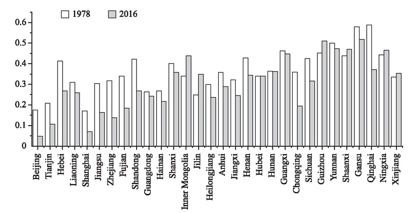
Industrial Structure Distortion Index by Region
5.2 Estimating the Impact of Industrial Structure Distortion Index on Energy Intensity
Common estimation methods for spatial econometric models are maximum likelihood (ML), quasi-maximum likelihood (QML), and instrumental variable (IV) methods (Anselin, 2008). We estimate the three spatial econometric models in the paper using the QML method. In the estimation, we consider space-specific effects to control the effects of unobservables that vary with space but not with time.
Because spatial econometric models use a complex dependency structure between sample units, changes in explanatory variables for a given unit potentially affect all other units in addition to the unit itself. In the case of this paper, the energy intensity of a province or region is affected not only by changes in its own ISD index but may also be affected by the index of ISDs in other provinces and regions. The first type of change is called the direct effect, while the second type of change is called the indirect effect. The total effect is the sum of direct and indirect effects. Table 2 gives the direct, indirect and total effects based on the estimations of models (15) ~ (17). [1] The first and second columns provide fixed and random effects estimates for the SAR model, the third column provides fixed effects estimates for the SAC model, and the fourth and fifth columns provide fixed and random effects estimates for the SDM model.
Direct, Indirect and Total Effects
| SAR_FE | SAR_RE | SAC_FE | SDM_FE | SDM_RE | |
|---|---|---|---|---|---|
| (1) | (2) | (3) | (4) | (5) | |
| Direct effect | |||||
| lnP | −0.156*** | −0.145*** | −0.144*** | 0.172** | 0.143* |
| (0.0248) | (0.0256) | (0.0249) | (0.0799) | (0.0758) | |
| lnd | 0.0004 | 0.0127 | 0.0072 | −0.0329 | −0.0212 |
| (0.0271) | (0.0279) | (0.0275) | (0.0253) | (0.0264) | |
| lnRD | 0.126*** | 0.120*** | 0.120*** | 0.174*** | 0.166*** |
| (0.0221) | (0.0225) | (0.0228) | (0.0200) | (0.0206) | |
| lnFDI | −0.0287 | −0.0372* | −0.0179 | −0.0424*** | −0.0498*** |
| (0.0179) | (0.0182) | (0.0195) | (0.0164) | (0.0168) | |
| lnTrade | −0.510*** | −0.498*** | −0.530*** | −0.479*** | −0.482*** |
| (0.0658) | (0.0664) | (0.0672) | (0.0609) | (0.0618) | |
| Indirect effect | |||||
| lnP | −0.480*** | −0.441*** | −0.553*** | −0.315** | −0.279* |
| (0.0988) | (0.0926) | (0.130) | (0.142) | (0.156) | |
| lnd | 0.0005 | 0.0385 | 0.0309 | 0.923*** | 0.942*** |
| (0.0864) | (0.0885) | (0.116) | (0.197) | (0.218) | |
| lnRD | 0.397** | 0.372** | 0.472** | −0.202* | −0.188 |
| (0.124) | (0.117) | (0.162) | (0.111) | (0.122) | |
| lnFDI | −0.0931 | −0.118 | −0.0691 | 0.309*** | 0.294*** |
| (0.0686) | (0.0683) | (0.0844) | (0.0679) | (0.0773) | |
| lnTrade | −1.590*** | −1.536*** | −2.099** | −1.310*** | −1.322*** |
| (0.409) | (0.382) | (0.678) | (0.367) | (0.401) | |
| Total effect | |||||
| lnP | −0.636*** | −0.586*** | −0.696*** | −0.143 | −0.136 |
| (0.110) | (0.106) | (0.136) | (0.125) | (0.140) | |
| lnd | 0.0007 | 0.0512 | 0.0381 | 0.891*** | 0.921*** |
| (0.113) | (0.116) | (0.142) | (0.200) | (0.222) | |
| lnRD | 0.523*** | 0.491*** | 0.592*** | −0.0287 | −0.0224 |
| (0.141) | (0.135) | (0.176) | (0.111) | (0.123) | |
| lnFDI | −0.122 | −0.155 | −0.0870 | 0.266*** | 0.244*** |
| (0.0855) | (0.0853) | (0.103) | (0.0696) | (0.0783) | |
| lnTrade | −2.099*** | −2.034*** | −2.628*** | −1.790*** | −1.804*** |
| (0.448) | (0.421) | (0.717) | (0.385) | (0.419) | |
| N | 510 | 510 | 510 | 510 | 510 |
Note: the explained variable is ln(E/Y); the numbers in parentheses are standard errors; *p < 0.1, **p < 0.05, and ***p < 0.01.
In the case of lnd, the core explanatory variable in this paper, the results in Table 2 indicate that its direct effect is greater than 0 in the first three regressions but not statistically significant, while that is less than 0 in the last two regressions and also not statistically significant. This implies that the ISD of a region does not have a significant direct effect on its energy intensity. The reasons for the statistically insignificant direct effects would be analyzed in the following part where we study the effects of sectoral distortions on energy intensity. In terms of indirect effects, the coefficient of the variable lnd is statistically insignificant in the SAR and SAC models, but it is 0.923 and 0.942 in the two estimates of the SDM model, respectively, which is highly statistically significant. Therefore, according to the SDM model estimation, the ISD has a significant negative impact on energy intensity through indirect effects. The total effect of the variable lnd is also insignificant in the SAR and SAC models but is significantly greater than zero in the SDM model. By considering the total effect of the SDM model, a 1% increase in the index of industrial structural distortion would ultimately increase energy intensity by 0.89%~0.92% overall.
The direct effect of the variable lnRD is highly statistically significant positive in the first three regressions, but highly statistically significant negative in the last two regressions. Its indirect effect is highly significant positive in the SAR and SAC models. While the indirect effect is negative in the SDM model, it is statistically significant in the SDM_FE estimate. The total effect is statistically significant positive in the estimates of SAR and SAC models. It is statistically insignificant in the two estimates of the SDM model, despite being negative. This result for the total effect suggests that R&D expenditure may not have reduced regional energy intensity in China. One possible reason is that, although R&D expenditure in China is growing rapidly, it is relatively inefficient. There is misallocation of public financial investment in innovation in particular (Wei et al., 2017). Also, the rapid growth of R&D expenditure reduces the resources (e.g., material capital and human capital) that would otherwise be available for producing goods and services in the context of budget constraints faced by enterprises. R&D investment has a crowding-out effect on investment in producing goods and offering services. In addition, when there is information asymmetry and government rent-seeking, government R&D incentives can lead to manipulative behavior of enterprises in R&D expenditure. Enterprises may strategically meet policy thresholds to obtain policy preferences, which ultimately reduces their R&D performance (Yang et al., 2017).
The direct effect of the variable lnFDI is negative in all five regressions, but statistically insignificant in the SAR_FE and SAC_FE estimates and statistically significant in the remaining three estimates. This unveils that, in most cases, FDI in a region helps to reduce its energy intensity. Its indirect effect is negative but statistically insignificant in the SAR and SAC models, while it is 0.309 and 0.294 in estimating fixed and random effects of the SDM model, respectively, and is highly statistically significant. The results from the SDM model show that, for a region, FDI attracted by other regions would have a significant negative impact on the energy intensity of that region. The reason may be that the growth of FDI inflows from other regions has a magnetic effect on the talent and capital of neighboring regions, thus negatively affecting the economic growth of neighboring regions. If the decline in neighboring output exceeds that in energy consumption, the energy intensity would rise. Finally, the total effect is also negative but statistically insignificant in the SAR and SAC models. The highly statistically significant estimates in the SDM model are 0.266 and 0.244, respectively, indicating that a 1% increase in FDI ultimately enhances energy intensity by 0.24%~0.27%. Therefore, although the inflow of FDI to a region may reduce its energy intensity through direct effects, the introduction of FDI does not have a positive effect on reducing its energy intensity through its technology spillover by considering the adverse effects of indirect effects.
The three effects of the foreign trade intensity variable lnTrade are highly significant negative in all regressions, suggesting that the development of foreign trade in a region can both contribute to its own reduction in energy intensity and have a positive effect on reducing energy intensity in other regions through spillover effects. Specifically, the direct effect ranges from −0.530 to −0.479 in the five regressions, indicating that a 1% increase in the share of a region’s foreign trade in GDP can reduce its energy intensity by 0.48%~0.53%. The indirect effect is also highly significant negative in the five regressions, ranging from −2.099 to −1.310. This indicates that, for a region, a 1% increase in the share of foreign trade in GDP in other regions can reduce the energy intensity of that region by 1.31%~2.10%. In the end, regarding the total effect, a 1% increase in the share of foreign trade in GDP can reduce energy intensity by 1.79%~2.63%, when other conditions are constant.
Finally, the direct effect of the energy price index variable lnP is statistically significant negative in the first three regressions but statistically significant positive in the last two regressions. However, the indirect effect is statistically significant negative in all five regressions. The total effect is also negative in all five regressions, but statistically insignificant in the last two regressions. Estimates of the total effect of the variable range from −0.696 to −0.136. When other conditions are constant, a 1% increase in energy prices can lead to an eventual reduction in energy intensity by 0.14%~0.70%.
5.3 Model Selection Test
Of the SAR, SAC, and SDM models, which would be more compatible with the sample data? First, according to the Hausman test, it is estimated that spatial fixed effects are preferable to random effects. Therefore, we perform model selection tests for three spatial fixed effect models: spatial autoregressive model for fixed effect estimation (SAR_FE), spatial Durbin model for fixed effect estimation (SDM_FE) and spatial autocorrelation model for fixed effect estimation (SAC_FE). Table 3 provides relevant test results. Since the SDM model is imbedded in the SAR model, the former can be turned into the latter when the coefficients of the spatially lagged explanatory variables are all zero. The LR test in the first row of Table 3 rejects the original hypothesis that the coefficients of the spatially lagged explanatory variables are all equal to zero. Therefore, the SDM model should be chosen through its comparison with the SAR model. Since the SDM model is not a nested form of the SAC model, we test the choice of the two models using AIC and BIC information criteria. According to the results in Table 3, the SDM_FE model has significantly smaller values of AIC and BIC than the SAC_FE model, indicating that the SDM_FE model is more compatible with sample data. In this way, section 6 summarizes the findings based on the SDM_ FE estimation.
Model Selection Test
| Model selection | Original hypothesis | LR test | p value | ||
|---|---|---|---|---|---|
| SDM_FE vs SAR_FE | Coefficients of all spatially lagged explanatory variables are zero | χ2 (5)=76.79 | 0.0000 | ||
| SAC_FE vs SDM_FE | Number of observations | Log likelihood value | Degree freedom of | AIC | BIC |
| SAC_FE | 510 | 455.26 | 8 | −894.52 | −860.64 |
| SDM_FE | 510 | 494.94 | 12 | −965.87 | −915.06 |
5.4 Impact of Sectoral Distortion Index on Energy Intensity
In this part, we estimate the QML for the SDM_FE model using the sectoral distortion index instead of the overall ISD index. The sectoral distortion index is calculated using the first equation in formula (13). The sectoral distortion indexes for the primary, secondary and tertiary industries are denoted as d1, d2 and d3. Since the sectoral distortion indexes for the secondary and tertiary industries are negative, this paper takes absolute and logarithmic values. Table 4 presents the direct, indirect and total effects of the QML estimations for the SDM_FE model. [1]
Direct, Indirect and Total Effects of Sectoral Distortion Index on Energy Intensity
| SDM_FE (6) | SDM_FE (7) | SDM_FE (8) | |
|---|---|---|---|
| Direct effect | |||
| lnd1 | 0.0325(0.0175** ) | ||
| lnd2 | −0.0431(0.0131*** ) | ||
| lnd3 | 0.0168(0.0066*** ) | ||
| Indirect effect | |||
| lnd1 | 0.808(0.148*** ) | ||
| lnd2 | 0.326(0.105*** ) | ||
| lnd3 | −(0.05950.0827 ) | ||
| Total effect | |||
| lnd1 | 0.841(0.152*** ) | ||
| lnd2 | 0.283(0.107*** ) | ||
| lnd3 | −(0.06150.0659 ) | ||
| N | 510 | 510 | 510 |
Note: the explained variable is ln(E/Y); the numbers in parentheses are standard errors; *p < 0.1, **p < 0.05, and ***p < 0.01.
Regression (6) in Table 4 reports the effect of the sectoral distortion index of the primary industry on energy intensity. It can be seen that the direct, indirect and total effects of the sectoral distortion index of the primary industry are highly significant positive in statistics. The total effect suggests that a 1% increase in the sectoral distortion index of the primary industry ultimately leads to a 0.84% increase in energy intensity, when other conditions are constant. Although the primary industry is a small part in output and energy consumption shares, the gap between the employment and output shares of the industry significantly worsens PTEI.
Regression (7) gives the effect of the sectoral distortion index of the secondary industry on PTEI. The results revealed that the direct effect of the sectoral distortion index on energy intensity is negative and highly statistically significant, but its indirect and total effects are highly significant positive in statistics. The value of the total effect reveals that a 1% increase in the sectoral distortion index of the secondary industry can ultimately increase the PTEI by 0.28%. Regression (8) reports the direct, indirect and total effects of sectoral distortions in the tertiary industry. With respect to the total effect, the sectoral distortions of the tertiary industry ultimately have no significant effect on PTEI.
Finally, we return to the question in Table 2 that the ISD index has no direct effect on energy intensity. Since the overall ISD index is an integrated result of sectoral distortions in the primary, secondary and tertiary industries, the direct effect of overall ISDs on energy intensity should also be an integrated result of the direct effect of distortions in the three industries. As can be seen in Table 4, the direct effects of the sectoral distortion indexes of the three industries almost cancel each other out and their combined effect is close to zero. This explains why the ISD index in Table 2 has no direct effect on energy intensity.
5.5 Robustness Test
The spatial weight matrix is changed in this paper to test the robustness of the estimated results of the spatial Durbin model for fixed effect (SDM_FE) in Table 2. We replace the spatial weight matrix of inverse Euclidean distance with the Queen adjacency space weight matrix and the 5th order nearest neighbor space weight matrix. Then, we re-estimate the SDM_FE. The estimated results are reported in Table 5. In both estimates, the direct, indirect and total effects of the variable lnd are positive and highly statistically significant in most cases, indicating the robust results of SDM_FE in Table 2.
Robustness Test
| I Queen adjacency weight matrix | ||||||
|---|---|---|---|---|---|---|
| Direct effect | Standard error | Indirect effect | Standard error | Total effect | Standard error | |
| lnP | −0.0502 | 0.0539 | −0.3785*** | 0.0675 | −0.4287*** | 0.0608 |
| lnd | 0.0568** | 0.0264 | 0.2627*** | 0.0750 | 0.3195*** | 0.0833 |
| lnRD | 0.1362*** | 0.0206 | −0.0610 | 0.0593 | 0.0752 | 0.0679 |
| lnFDI | −0.0142 | 0.0161 | 0.2239*** | 0.0430 | 0.2097*** | 0.0499 |
| lnTrade | −0.5153*** | 0.0646 | −0.7716*** | 0.2131 | −1.2868*** | 0.2506 |
| II 5th order nearest neighbor weight matrix | ||||||
| Direct effect | Standard error | Indirect effect | Standard error | Total effect | Standard error | |
| lnP | −0.0849 | 0.0756 | −0.1995** | 0.0940 | −0.2844*** | 0.0733 |
| lnd | 0.0252 | 0.0152 | 0.4407*** | 0.1101 | 0.4659*** | 0.1192 |
| lnRD | 0.1758*** | 0.0199 | −0.1290* | 0.0760 | 0.0469 | 0.0830 |
| lnFDI | −0.0350** | 0.0158 | 0.2346*** | 0.0557 | 0.1995*** | 0.0621 |
| lnTrade | −0.4464*** | 0.0628 | −0.7411*** | 0.2746 | −1.1875*** | 0.3090 |
Note: the explained variable is ln(E/Y); *p < 0.1, **p < 0.05, and ***p < 0.01.
6 Conclusions and Recommendations
We first studied the impact of technological progress on industrial structure changes based on Nunn and Qian (2011). Then, we measured the ISD index for 30 provinces (municipalities) in mainland China excluding Xizang from 1978 to 2016 using Ando and Nassar (2017). Finally, we used relevant data from 1998 to 2014 based on a spatial panel econometric model to analyze the impact of the ISD index on energy intensity. The relevant conclusions can be summarized as follows.
First, between 1978 and 2016, the 30 sample provinces and regions as a whole experienced an overall significant decline in their ISD index. The ISD index decreased from 0.4987 in 1978 to 0.2348 in 2016, with the efficiency of allocation of labor resources in the three industries improved significantly. Second, the SDM_ FE estimation suggest that while industrial structural distortions do not have a significant direct effect on energy intensity, they have a significant adverse effect on reducing energy intensity through indirect effects. Specifically, a 1% increase in the ISD index ultimately results in a 0.89% increase in energy intensity. Third, the energy price index is an important factor declining energy intensity. The total elasticity of energy intensity with respect to the energy price index is −0.143 in the SDM_FE estimation. In other words, when other conditions are constant, a 1% increase in energy price would reduce China’s energy intensity by 0.143%. Fourth, foreign trade is the most important factor declining China’s energy intensity. The introduction of FDI worsens energy intensity, while R&D investment has no significant effect on energy intensity.
Based on the above findings, we propose the following policy recommendations from the perspective of eliminating the ISD and reducing energy intensity. First, the micro cause of ISD are market imperfection and government policy preference. It is required that we should make up the huge differences between urban and rural residents in education, healthcare, employment, elderly care and other public services, remove the barriers that restrict agricultural labor from working in urban areas, and facilitate the integrated development of urban and rural areas. We should promote reforms in the household registration, compulsory education, employment, pension and healthcare systems that meet the requirements of new urbanization to expedite the continued transfer of agricultural labor to industrial and urban sectors. Also, more government investment in all levels and types of education should further improve the educational level of the workforce. We should improve the knowledge of the workforce to help promote its cross-sectoral mobility across regions and enhance the efficiency of sectoral allocation of labor resources, thus contributing to reducing the ISD.
Second, the highest ISD is found in the western region, while the impact of structural distortion of primary, secondary and tertiary industries on energy intensity gradually decreases. In the future, the government should focus on the western region from the perspective of industrial structure optimization to accelerate the substitution of emerging industries for traditional industries and the elimination of outdated production capacity, and rationally allocate production factors. In the “post-industrialization” stage, the proportion of high-tech and service-oriented industries in the national economy should be gradually increased, new driving forces of green economic development should be fostered, and the inhibiting effect of ISD on reducing energy intensity should be effectively alleviated.
Energy price is an important factor declining energy intensity. Reform of the energy price formation mechanism should be promoted to give play to the decisive role of market in allocating resources. Currently, except for the market-oriented coal price, prices of some energy products are subject to relatively strict government regulation. As such, energy prices do not fully reflect market supply and demand and the scarcity of resources, nor do they reflect the environmental costs of energy use. China should continue to implement its market-oriented reform of energy price formation mechanism, push forward the reform of the price system for refined oil, natural gas and electricity, and establish a price formation mechanism for oil, gas and electricity that is determined by the market but effectively regulated by the government. It should use the price mechanism to regulate energy supply and demand and promote energy saving and emission reduction efforts.
Finally, R&D investment has not had the expected pro-reduction effect on energy intensity. China should improve the allocation mechanism of public R&D expenditures, while enhancing the efficiency of the R&D sector’s activities. China is currently seeing rapid growth in public R&D expenditure, but there may be a misallocation of resources among sectors and enterprises. In particular, government R&D incentives induce strategic behavior of enterprises in R&D expenditure, while the government makes public R&D expenditure more biased towards state-owned enterprises, thus reducing the utilization efficiency of R&D expenditure. The efficiency of R&D activities can be improved as soon as possible, which represents an urgent issue for the Chinese government to implement the innovation-driven development strategy.
References
Ando, S., & Nassar, K. (2017). Indexing Structural Distortion: Sectoral Productivity, Structural Change and Growth. IMF Working Paper, WP/17/205.10.5089/9781484319277.001Search in Google Scholar
Anselin L., Le Gallo, J., & Jayet, H. (2008). Spatial Panel Econometrics. In: Matyas, L., & Sevestre, P. (eds), The Econometrics of Panel Data: Fundamentals and Recent Developments in Theory and Practice, 3rd edn. Dordrecht: Kluwer, 901−969.10.1007/978-3-540-75892-1_19Search in Google Scholar
Drukker, D. M., Peng, H., & Prucha, I. R. (2013), Creating and Managing Spatial-weighting Matrices with the Spmat Command. The Stata Journal, 12(2), 242−286.10.1177/1536867X1301300202Search in Google Scholar
Elliott, R., Sun, P., & Chen, S. (2013), Energy Intensity and Foreign Direct Investment: A Chinese City-Level Study. Energy Economics, 40(1), 484−494.10.1016/j.eneco.2013.08.004Search in Google Scholar
Golder, B. (2011), Energy Intensity of Indian Manufacturing Firms: Effect of Energy Prices, Technology and Firm Characteristics. Working Papers, (3), 351−372.10.1177/097172181101600306Search in Google Scholar
Hang, L., & Tu, M. (2007). The Impacts of Energy Prices On Energy Intensity: Evidence From China. Energy Policy, 35, 2978−2988.10.1016/j.enpol.2006.10.022Search in Google Scholar
Howitt, P. (1999). Steady Endogenous Growth with Population and R&D Inputs Growing. Journal of Political Economy, 107(4), 715−730.10.1086/250076Search in Google Scholar
Ju, K., Su, B., & Zhou, D. (2017). Does Energy-Price Regulation Benefit China’s Economy and Environment? Evidence From Energy-Price Distortions. Energy Policy, 105(JUN), 108−119.10.1016/j.enpol.2017.02.031Search in Google Scholar
Kuznets, S. (1971). Economic Growth of Nations. Cambridge: Harvard University Press.10.4159/harvard.9780674493490Search in Google Scholar
Liao, H., Fan, Y., & Wei, Y. (2007). What Induced China’s Energy Intensity To Fluctuate: 1997−2006? Energy Policy, 35(9), 4640−4649.10.1016/j.enpol.2007.03.028Search in Google Scholar
Lin, B., & Du, Z. (2017). Promoting Energy Conservation in China’s Metallurgy Industry. Energy Policy, 104 (MAY), 285−294.10.1016/j.enpol.2017.02.005Search in Google Scholar
Ma, C., & Stern, D. (2008). China’s Changing Energy Intensity Trend: A Decomposition Analysis. Energy Economics, 30 (3), 1037−1053.10.1016/j.eneco.2007.05.005Search in Google Scholar
Nunn, N., & Qian, N. (2011). The Potato’s Contribution to Population and Urbanization: Evidence from a Historical Experiment. The Quarterly Journal of Economics, 126 (2), 593−650.10.3386/w15157Search in Google Scholar
Tan, R., & Lin, B. (2018). What Factors Lead to the Decline of Energy Intensity in China’s Energy Intensive Industries? Energy Economics, 71(2), 213−221.10.1016/j.eneco.2018.02.019Search in Google Scholar
Wei, S., Xie, Z., & Zhang, X. (2017). From “Made in China” to “Created in China”. Comparative Studies (Bijiao), 3, 15−37.Search in Google Scholar
Wu, Y. (2012). Energy Intensity and Its Determinants in China’s Regional Economies. Energy Policy, 41, 703−711.10.1016/j.enpol.2011.11.034Search in Google Scholar
Yang, G., Liu, J., Qian, P., & Rui, M. (2017). Tax-Reducing Incentives, R&D Manipulation and R&D Performance. Economic Research (Jingji Yanjiu), 110−124.Search in Google Scholar
Young, A. (1998). Growth without Scale Effects. Journal of Political Economy, 106 (1), 41−63.10.3386/w5211Search in Google Scholar
Yu, H. (2012). The Influential Factors of China’s Regional Energy Intensity and Its Spatial Linkages: 1988−2007. Energy Policy, 45, 583−593.10.1016/j.enpol.2012.03.009Search in Google Scholar
Zheng, Y., Qi, J., & Chen, X. (2011). The Effect of Increasing Exports on Industrial Energy Intensity in China. Energy Policy, 39, 2688−2698.10.1016/j.enpol.2011.02.038Search in Google Scholar
© 2021 Xiaobo Shen, Yu Chen, Boqiang Lin, published by De Gruyter
This work is licensed under the Creative Commons Attribution 4.0 International License.
Articles in the same Issue
- Frontmatter
- Research on the Scientific Connotation of New Development Pattern
- Impact of Technological Progress and Industrial Structure Distortion on Energy Intensity in China
- Impacts of Property Tax Levy on Housing Price and Rent: Theoretical Models and Simulation with Insights on the Timing of China Adopting the Property Tax
- Has Global Division of Labor Increased Markup of Chinese Enterprises?
- Digital Economy Development, International Trade Efficiency and Trade Uncertainty
- Make Coordinated Efforts to Advance the Building of Modern Circulation System in the Context of the New Development Pattern