
Transaction Costs and Institutions: Investments in Exchange
-
Charles Nolan


Abstract
This paper proposes a simple model for understanding transaction costs – their composition, size and policy implications. We distinguish between investments in institutions that facilitate exchange and the cost of conducting exchange itself. Institutional quality and market size are determined by the decisions of risk adverse agents and conditions are discussed under which the efficient allocation may be decentralized. We highlight a number of differences with models where transaction costs are exogenous, including the implications for taxation and measurement issues.
1 Introduction
Models that incorporate transaction costs generally treat them as a “useful formalism” (Townsend 1983). They are meant to capture the costs of collecting information, of bargaining, organization, decision making, writing and enforcing contracts between individuals, firms and the state (Coase 1960). The perception of such costs as exogenously impeding trade or inhibiting the formation of complete contracts suggests that reducing, eliminating or avoiding those costs is generally welfare enhancing.[1] As the quality of institutions is thought to be a part of what explains those transaction costs,[2] the implication is that better institutions always improve economic outcomes.
Many of these transaction costs are not directly impeding trade, however, but are resources allocated to technologies (or institutions) that facilitate exchange, even though those resources could otherwise have been allocated directly to the production of a consumption good. For example, the organization of the firm, the formation and nature of contracts, the emergence and use of a legal system are all themselves technologies employed to ease the conduct of exchange. Investments in such technologies – in the form of legal or judiciary arrangements, management consultants, and so on – are investments in an “institutional capital”. The consequence of such investment is that the cost of an individual exchange can be lower. For example, the expected loss from a trade may be reduced, or it may be less costly to assess the quality of a traded good, if we have established standardized reporting practices; an economy with a stronger contracting environment can limit the losses from opportunistic behaviour in trading; and so on. Moreover, the investments in exchange technologies can be private or public. Private investment in such capital could involve the formulation of trading standards within a coalition of traders, for example: There is an upfront cost to establishing and enforcing those standards but these may lower intermediation costs because trading risk is reduced. Public investment may be improvements in property rights legislation that make the transfer of assets more secure; again, such improvements are costly but they may reduce the costs of individual trades if it leads to fewer losses from disputed exchanges. Each of these costs may be categorized as “transaction costs” but they can serve quite different purposes: Some are investments that facilitate exchange; some, such as trading risk or legal fees, are the subsequent costs of exchange.
We develop a model in which risk-averse agents who do not know their own production technology may, in advance of the productivity realization, form a coalition to share consumption risk. Agents face a cost to exchange output, however, and that cost of exchange is determined by investment in exchange cost-reducing institutions. Total transaction costs are then the sum of two components: There is a cost to forming the public and private institutions that govern, ex ante, the terms of exchange, and there are costs to conducting exchange once the state of nature is resolved.[3] Agents choose the resources allocated to reducing exchange costs and the extent of diversification (how extensively they will trade with others).
A number of results follow from modelling transaction costs as an endogenous component of a general equilibrium set-up. We first characterize the optimal allocation. Naturally, while the costs of exchange can be too high, they can also be too low. A high exchange cost reflects fewer resources directed towards facilitating transactions but may be associated with greater expected utility if those free resources are put to productive use and if agents choose to make fewer costly exchanges. Understanding these issues is directly important for policy design since many public institutions, such as the legal system, are bound up in the costs of trade. Real-world policies are generally based around simple objectives such as maximizing the size of markets or minimizing the cost of an individual exchange. Given the absence of a framework in which to account for the general equilibrium consequences of transaction costs, we cannot understand the welfare-ranking of different simple policies. Having established the optimal allocation, and since our model can be considered quantitatively, we can conduct such an analysis.
By far the most damaging type of simple policy, in welfare terms, is one that focuses on minimizing the costs of individual exchange. The intuition is as follows: The optimal allocation represents a trade-off between the portion of the endowment that goes to production (i.e., net of transaction costs) and the amount of consumption variability. The minimum-exchange cost policy is so damaging because it ignores both consumption variability and the overall costs of transactions. A policy that targets market size is less damaging since it minimizes the overall consumption variability and allows agents to respond in their private investment decisions. The least damaging of the simple policies we consider is a policy which minimizes the overall size of the transaction sector. Under this policy, agents can respond to deviations from an optimal tax policy by varying both the amount they trade and their private investments in exchange.
In addition to policies that distort allocations to the institutional capital, we also consider the effect of a transactions tax. Agents invest more in institutions to ameliorate the effect of the tax on the costs of exchange, thereby making diversification decisions less sensitive to increases in the transactions tax. However, while apparently robust to the imposition of a transaction tax, agents opt for autarky at a lower transaction tax than might be anticipated using a model of exogenous transaction costs.
We can also use our quantitative model to put the empirical evidence on transaction costs into some context. Coase (1992, 716) argues that “a large part” of economic activity is directed at alleviating transaction costs. In a first attempt to quantify the aggregate extent of such resources, Wallis and North (1986) estimate that what they term the transaction sector comprised half of US GNP in 1970, a proportion which had grown significantly over the preceding century. Moreover, Klaes (2008) concludes that economies with less sophisticated transaction sectors appear, at an aggregate level, to exhibit lower levels of transaction costs. In our model, a more wealthy economy is characterized by a smaller transaction sector, but one based on greater investments in institutions, larger markets and lower exchange costs. This is consistent with the evidence in Klaes (2008), that, at a micro-level, the costs of exchange are high when the aggregate transaction sector appears to be small.
Our framework relates to a number of other papers. The idea that investments in better transaction technologies can be part of an efficient economic system has been put forward by De Alessi (1983), Barzel (1985) and Williamson (1998). In making transaction costs endogenous, we are also blurring the distinction between institutional and technological efficiency, as Antras and Rossi-Hansberg (2009) have noted in a survey on organizations and trade. In that literature, decisions on organizational arrangements and on trade are interrelated. In our approach, agents make joint-decisions about their productive capacity, risk sharing and the investments in institutions that govern the costliness of trade. Finally, the gains from allocating resources to institutions relate to the idea of a “state capacity” in Besley and Persson (2010). State capacity is partly “legal infrastructure investments such as building court systems, educating and employing judges and registering property or credit”(p. 6). In that model, equilibrium investments in legal capacity are increasing in national income. Our approach also considers the possibility of a “private capacity” that might substitute for or complement investments in public institutions.
The model is set out in Section 2. Section 3 characterizes efficient equilibria, that is the optimal investment in institutional capital, the optimal extent of transaction costs and the optimal market size. The conditions are discussed in Section 4 under which the efficient equilibrium may be decentralized. Section 5 reports the implications of our model in the lights of extant empirical evidence. Section 6 examines the impact of (simple) non-optimal institutions and also looks at the impact of an exogenous transaction tax. Having established the efficient allocation in Section 3, we can compute the welfare cost of each of these policies. Section 7 summarizes and concludes. Appendices contain some proofs, further numerical analysis of the model and a detailed description of the decentralized equilibrium.
2 The Model: Overview
We briefly outline the model (which is motivated by Townsend 1978) before presenting it in detail. A large number of risk averse agents are each endowed with the same amount of capital. That capital can be combined with a production technology to produce a consumption good. Agents can differ in the technology with which they can produce the consumption good but, initially, they know only the distribution of possible technologies. Consumption risk can be reduced by forming markets with other agents but due to exchange costs it is not feasible to replicate a complete Arrow-Debreu allocation. The cost of each bilateral exchange is determined in a simple way by the quality of contracting institutions in the economy. As such, before they realise their productivity, agents decide whether or not to form a market with other agents and, if they do, how large that market should be and how much to invest in private (i.e., excludable) and public institutional quality.[4]
One agent per market becomes an intermediary, buying outputs and selling consumption bundles. Intermediaries are here the productive unit of the transaction sector, using the institutional capital as input to a common “exchange cost technology” (ECT), the output of which is the exchange cost incurred by agents in its market. Ex post, agents honour their obligations even if it would be preferable to renege. If agents do not join a market then no institutional investment takes place. The primary aim of Sections 3–4 is to characterize the efficient level of institutional capital, exchange costs and market size (consumption risk sharing) for such a model economy.
2.1 Preferences and Production Technology
The economy is populated by a countable infinity of agents,
Let
2.2 Diversification and Intermediation
To diversify against risk, agents can form markets in a star network around a single intermediary, as in Townsend (1978). A market is a set of agents
Agents can exchange some of their endowment of capital on a one-for-one basis for shares in the consumption portfolio compiled by the intermediary, less their contributions to the total costs of transactions. Each agent in a market exchanges twice with the intermediary and pays an equal share of market-wide exchange costs. So for a given exchange cost,
2.3 Institutional Capital and Exchange Costs
Intermediaries form markets using institutional capital as an input to an exchange cost technology (ECT) which determines the cost of exchange in that market. There is free-entry to intermediation (i.e., the ECT is accessible to all agents). Institutional capital takes two forms: There is a market-specific institutional capital (
In a market intermediated by agent
where
Since the intention of this paper is to explore the general equilibrium implications of agent investments in reducing exchange costs, the equation for the exchange cost,
First, we may consider the transaction cost to the be product of the “transfer of property rights” (Allen 2000, 901). That is, there are frictions associated with a transaction because of the “costs of bookkeeping, the cost of enforcement, the cost of monitoring…” (Townsend 1983, 259). That “cost” is related, however, to the institutional capital from which the agents in the exchange can draw; the form of eq. [1] imposes a natural relationship between investments in that institutional capital and the consequent cost of conducting exchange. The cost of enforcing a contract is a product of the quality of the legal system, for example. Consider, for example, the problem of trading an item of unknown quality. This mechanism can be motivated using an example in Langlois (2006). Prior to the coming of the railroad to the American Midwest in the mid-nineteenth century, the trade of grain could be conducted on a personal basis with quality levels maintained through the observed reputation of individual farmers. Once the railroads vastly increased the scale of trade, individual farmer grains became mixed and the grains were traded as commodities in a way detached from their original producer, thus breaking the prior system of quality control. In response, the Chicago Board of Trade (CBOT) was formed to standardize the nature of the grain trade. Setting up such standards was costly but there were also continuing costs of inspecting each transaction for conformance. The CBOT reduced the risks involved in making an individual exchange of grain, reducing the margin required by traders engaged in buying and selling grain.
A second perspective is one of incomplete contracts, i.e., that transaction costs are “the costs of establishing and maintaining property rights” (Allen 2000, 898). Hart and Moore (2008) introduce a model in which the broad outlines of trade may be defined ex ante. Ex post, there are costs to fill in the detail of the finer points. A contract embodies a trade-off between flexibility and rigidity in which an optimal arrangement may not be fully specified over all possible states of nature. For Hart and Moore (2008), the costs from such partial incompleteness can take the form of a deadweight loss. We may also think of this in the context of complexity (cf. Anderlini and Felli 1999). In the context of our model, goods may be produced with different technologies that require specific contracts that are complex (costly) to write. To write ex ante contracts for each possible technology would be exorbitantly expensive, but to write no contracts ex ante would mean that, ex post, there would be no trade. Ex ante investments in legal and accounting systems could mean that agents are committed to trade under the rough outlines of an agreement, leaving the costs of writing specific contracts for individual trades to be incurred after the state of the world is known.
The distinction between the specific and general determinants of the costs of exchange also emerges from this literature. Williamson (1979) refers to the “governance of contractual relations”. Anderlini and Felli (1999) consider that some of what determines the extent of complexity costs is environmental, since a contract is “‘embedded’ in a larger legal system” (Anderlini and Felli 1999, 25). A second determinant is specific to the market in which the contract is formed. The distinction between
Each type of institutional capital may impact upon the other in determination of exchange costs. In our baseline case, we assume that
3 Efficient Equilibria
The purpose of this Section is to characterize efficient allocations in a cooperative setting; i.e., in an economy where intermediaries arise exogenously and where there is no difficulty providing the public good,
An intermediary
subject to,
Equation [3] limits consumption to be less than or equal to output in each state of nature, on a market-wide basis. Equation [4] says that, in any market, the sum of endowments net of production and institutional investment must be sufficient to cover the total of market exchange costs. Equations [5] and [6] describe institutional capital, eq. [7] restricts the range of feasible
then no intermediated market with exchange is formed (i.e.,
3.1 Optimality
All agents share an aliquot consumption payout in each market as determined by the observed average technology for that market,
Equation [10] ensures that there exists a
For each
The relevant measure space is given by the triple
Decisions on
For each
need not be unique. Finally, the equivalence between the cooperative case and core allocations is established in Proposition 5.■
Some properties of efficient equilibria are immediate. Since the ECT is freely accessible, rents from intermediation must be zero so eqs [5] and [6] hold with equality. The optimal allocations to the ECT is the pair
where
Clearly, the optimal market size is unity,
Remark 1 follows from analysis of eqs [14] and [15]:
For
The choice of any market size greater than one is determined by the ECT and agents’ attitude to risk. Equations [14] and [15] determine efficient investment in the ECT and hence total resources diverted from goods production. Agents’ risk aversion provides an upper bound on how much they are willing to pay for consumption insurance, given an alternative not to diversify; that bound is independent of the ECT. Agents will optimally form markets with
The rest of the analysis of equilibrium is contained in the following four Propositions. One can show that in general there is a critical level of
There is a
See Appendix A.1.■
The key to understanding that Proposition is to recall that
Proposition 2 also indicates the possibility of multiple optimal plans. Proposition 3 now shows that no more than two such alternative plans can exist.
The optimal policy correspondence contains at most two plans.
See Appendix A.1.■
As a corollary, it follows that for any
Let
where
See Appendix A.1.■
The set of values of
To summarize: Low endowment economies may resort to autarky (Proposition 2). However, for economies with larger endowments (
The allocations of the cooperative economy coincide with core allocations.
See Appendix A.1.■
4 Equilibrium with Competitive Intermediation
The question now is: Can the efficient outcome be decentralized? First, note that given the public good nature of the
In the core, voluntary allocations to general capital are zero.
See Appendix A.2.■
There are a number of ways in which the public good problem inherent in
We formalize this perspective and consider the outcome to be the result of a market with free-entry: Any agent can costlessly seek a mandate that specifies taxes for all agents and the level of
If any agent may propose an enforceable tax plan then all agents will be taxed according to eq. [15]. It follows that
See Appendix A.2.■
There is no such problem in the provision of
If the public good is provided according to Proposition 7, the provision of
See Appendix A.3.■
5 The Size of the Transaction Sector
The empirical literature on transaction costs has focused on the costs of individual transactions or individual organizational arrangements. Insofar as they can be measured, the size of such costs is considered a measure of the working of the market. Examples in a variety of different contexts, from property rights to finance, are noted in Allen (2000). In contrast to the study of individual transactions, there has been limited work to establish the size of transaction costs on aggregate. Wallis and North (1986) were the first to quantify the size of the US transaction sector. By dividing occupations into those classified as providing “transaction services” to firms and those that provide primarily “transformative” services, Wallis and North calculate the total remuneration to transaction occupations. This sum constitutes the size of the transaction sector. They found that in 1870, the transaction sector accounted for 25% of GNP, rising to 50% in 1970.[12] The Wallis and North methodology has been applied to Australia (Dollery and Leong 2002), Bulgaria (Chobanov and Egbert 2007) and New Zealand (Hazledine 2001) with similar magnitudes and trends found in each.
We thus have two observations from different empirical literatures on transaction costs: First, the size of the transaction sector is large and positively related to wealth; and, second, low transaction costs are one of the spurs of development.[13] The model presented here offers a natural way to consider both observations and to suggest directions for future empirical work. As we have defined them, transaction costs are composed of the costs of making individual exchanges and the investments in exchange institutions. Our model, then, hinges on a distinction between ex ante and ex post costs which is not a focus of empirical study. However, we take the empirical evidence on individual arrangements to reflect an individual ex post exchange cost (
We let
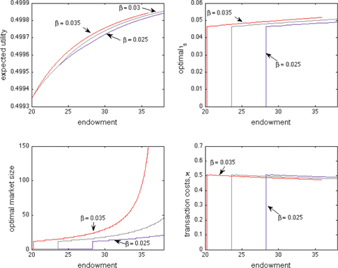
Some comparative static results are intuitive. Suppose that at some
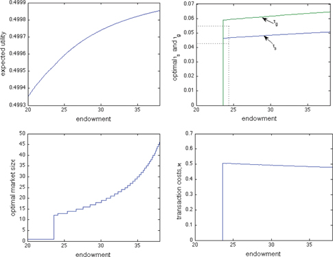
Equilibrium over a range of the endowment.
Proportionate investments in institutions can increase in
These numerical results are robust to varying a number of different parameters, as shown in Appendix A.5. The coefficient or relative risk aversion drives the extent of diversification but, so long as it does not shut down all exchange, its impact on
6 The Impact of Non-optimal Public Institutions
So far the analysis has focused on the nature of efficient equilibria; the efficient tax level,
6.1 Equilibrium with Exogenous τ g
The distortive behaviour centres on the resources turned over to
Figure 2 reports the consequences of varying
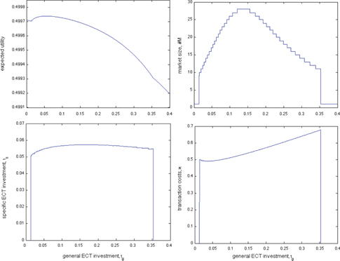
Equilibrium with distortive institutions.
At very low levels of
Given that Section 11 has established the efficient outcome, we can calculate the consumption equivalent loss for each level of
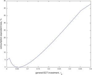
Welfare costs of distortionary institutions.
6.2 Specific Transaction Cost Policies
The discussion of the empirical evidence above points to the complexity of classifying and measuring transaction costs in reality. In the light of that, it is reasonable to consider an environment where the optimal tax policy is unclear. The literature on transaction cost economics suggests that optimality is where “transactions are aligned with governance structures so as to effect a (mainly) transaction cost economizing outcome” (Williamson 2010, 681). The interpretation of that optimality condition in terms of policy may be complicated since there are multiple observable and potentially non-observable components: The number of exchanges (market size), the investments in reducing the cost of exchange, and the cost of exchange itself. As such, a policy maker may have as its objective some minimum or maximum of each of these and think it a reasonable interpretation of what is optimal: First, institutions could deliver zero exchange costs; second, institutions should maximise risk-sharing; third, the cost of individual exchanges should be minimized[18]; and, fourth, institutions should minimize the size of the transaction sector as a whole.
In our model, zero exchange costs are not feasible; institutions which deliver an infinite number of trades at zero cost are themselves infinitely costly. However, the analysis above shows that we can consider the second, third and fourth type of policy prescription. The second is a rule that maximizes the (constrained optimal) choice of market size; the third minimizes the cost of individual exchanges; the fourth minimizes size of the transaction sector. The market size policy is given by,
That is,
Finally, the tax policy which minimizes the transaction sector is given by,
For each policy the percentage change in certainty equivalent consumption is calculated using the efficient frontier established in Section 3. Table 1 describes various features of equilibrium under the different rules.
The effects of distortive institutions.
| Rule | ||||||
| 18 | 0.4940 | 0.0550 | 0.0550 | 6.0795 | – | |
| 28 | 0.5234 | 0.1210 | 0.0571 | 5.3711 | 4.3368 | |
| 11 | 0.6781 | 0.3520 | 0.0548 | 4.4776 | 38.2895 | |
| 14 | 0.4906 | 0.0376 | 0.0537 | 6.4502 | 0.6400 |
None of the rules are optimal in a framework with endogenous transaction costs; the
The loss from
6.3 Transaction Taxes
Policies are sometimes designed to address the negative externalities from trade (such as trades of a pollutive item), or to raise revenue from a sector characterized by high-frequency trading (as in a Tobin-type tax). In such policies, individual exchanges are taxed. The European Commission analysis of its proposed Financial Transaction Tax (FTT), for example, finds “in a nutshell… very positive impacts on the functioning of the single market for financial instruments” (European Commission 2013, 16). The consequences of such a tax are not necessarily obvious; however, since agents may respond by increasing investment in private exchange cost reduction or may dramatically change the number of trades. Moreover, the robustness of a market to the imposition of a tax, i.e., its revenue-generating ability, may not be fully understood since those markets may shut down or relocate to avoid the tax.
In order to understand the impact of a transaction tax, we need a framework in which the nature of trade (i.e., the number of exchanges and investments in the cost of exchange) is endogenous. As such, our model can form a basis for a preliminary analysis of transaction taxes. We can consider a tax,
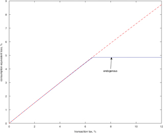
Figure 4 demonstrates the effect of a transaction tax where transaction costs are endogenous (solid line). Agents respond first by increasing investments in institutions in order to dampen the effect of the tax on the cost of exchange. Relative to an environment where transaction costs are exogenous (dashed line),[20] market size is more robust to the introduction of a transaction tax. In each environment, agents can avoid the tax by simply resorting to autarky, recovering the investment in exchange and avoiding all tax, whenever the participation constraint is no longer satisfied. The important difference when transaction costs are endogenous is that agents have individually allocated a portion of their endowment to support institutions; in the exogenous case this investment has not occurred and so cannot be retrieved by agents. That means that although agents initially appear less affected by the tax, they will opt for autarky at a level of the tax far lower than that suggested when transaction costs are considered exogenous.[21] The implication for transaction tax policy is that, while markets respond as would be expected to the imposition of a tax by reducing market size, agents will resort to autarky earlier than may expected if the individual agents’ own investments in that exchange are not taken into account. In case of the FTT, for example, this may mean that a transaction tax leads to the shifting of financial activities to geographies outwith the FTT’s jurisdiction at much lower levels of the tax than may be anticipated. Revenues from such a tax may fall short of projections.
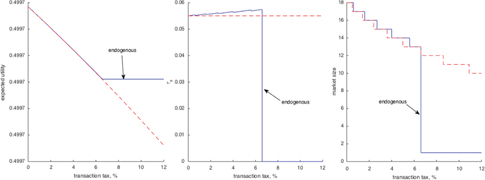
The effects of a transaction tax.
We can again calculate the losses from imposing a tax on transactions. Figure 5 depicts losses associated with Figure 4. A 5% transaction tax leads to 3.7% consumption equivalent loss in both the exogenous and endogenous cases, which is somewhat higher than an equal deviation in the
Welfare costs of transaction taxes.
7 Discussion and Concluding Remarks
Economists are increasingly focusing on the role of good institutions in promoting growth, trade and other desiderata. The intention of this paper is to link in a simple way impediment to transactions, institutional quality and market size. The efficient equilibrium of the model is consistent with significant transaction costs and investments in institutions. A distinction between transaction costs and exchange costs was made. The impact of distortive institutions was also considered, although in a tentative and ultimately ad hoc way. We argued that a number of what might be thought of as “good” institutions is actually sub-optimal when transaction costs are endogenous.
It would seem important to extend the analysis in a number of directions. First, although agents had different productive capabilities, this had a limited impact as decisions over
Acknowledgement
We are grateful to the editor and three referees for comments that have improved this paper. We thank colleagues at the Universities of Edinburgh, Exeter, Koç and St. Andrews, and also at the RES Conference at Warwick University and the ISNIE Conference in Toronto. In particular, we thank, without implicating, Sumru Altug, Vladislav Damjanovic, John Driffill, Oliver Kirchkamp, John Moore, Helmut Rainer, József Sákovics, David Ulph and especially Tatiana Damjanovic, Daniel Danau and Gary Shea.
Appendix
A.1 Proofs of Section 3 Propositions
There is a
To the contrary, assume that
for all
As
The optimal policy correspondence contains at most two plans.
Let
Now, denote
where
By assumption
that is, market size associated with
Let
where
Let
Hence
for
Following Townsend (1978) and Boyd and Prescott (1985) one may characterize core allocations directly. In the discussion of the efficient equilibrium in the main text we studied the equilibrium decision rules of an intermediary. Townsend (1978) labelled that analysis the “cooperative” solution. Hence, the equivalence of the core and cooperative solutions is now established, Proposition 5 in the text.
The allocations of the cooperative economy coincide with core allocations.
Consider the unique equilibrium:
The consumption profile follows from optimizing over agents with identical, strictly concave utility functions and the second condition was derived in the text. By Remark 1,
A.2 Proofs of Section 4 Propositions
In the core, voluntary allocations to general capital are zero.
Consider an equilibrium in which
If any agent may propose an enforceable tax plan then all agents will be taxed according to eq. [15]. It follows that
Suppose that a group of agents
A.3 Proof of Proposition 8
The equivalence of core and competitive equilibria is established by extending the arguments of Townsend (1978). First, some notation is developed. Let any agent
A competitive equilibrium is a set of actions
There exist no blocking strategies for any agent of
Hence, a non-intermediary faces the following problem:
subject to the following constraints regarding feasibility and participation,
An intermediary chooses a strategy to maximize,
subject to,
and the following relations:
Equation [35] may be regarded as the free-entry constraint upon the equilibrium intermediary strategy.
If there exists a competitive equilibrium, with political free-entry as defined above, then the equilibrium is in the core.
Consider an equilibrium, for a given endowment k, for which a blocking coalition exists. Further, assume that this blocking coalition, denoted
where
where
and,
Therefore,
Finally, we have,
Since they are the shadow prices of dual constraints, it follows
Equation [47] determines the unique optimal,
If this agent is a non-intermediary this follows from
All core allocations can be supported as equilibria.
Assume that the optimal market size is greater than unity and less than infinity. Then the above first-order conditions can be used directly to construct an equilibrium that is a competitive equilibrium (since core and competitive equilibria coincide). Since the optimal market size exists, one may construct equilibrium markets. Hence, Properties 1 and 2 of the definition of equilibrium are met. Finally, no set of agents will block this allocation since it would be unable to attain a higher level of utility than under the cooperative equilibrium.■
A.4 Comparative Static Results
Remark 1 shows that market size and ECT allocations increase in
For a given market size greater than one, (i) transaction costs are strictly decreasing in
Transaction costs: Recall
where
ECT investment: Throughout, it is assumed that
It should be recalled that we are characterizing optimal outcomes for a given
Equation [52] allows one to check the sign of the elasticity;
A.5 Numerical Solution to the Model
First, the choice of functional form for the ECT and utility function is discussed, as is the modelling of consumption-good productivity. Next, the solution of the model is explained and analysed holding fixed the level of the endowment. The solution of the model is then studied when
A.5.1 A Numerically Tractable Model
Consider a general CES form for the ECT,
where
where
The Inada-type requirements are readily confirmed. In addition, the parameters
Agents have identical CRRA utility,
The expected average technology for a market of size
which is invariant to
subject to
where
A.5.2 ECT, Diversification and Utility with a Fixed Endowment
Table 2 gives the parameter values in the baseline case.
Baseline calibration for endogenous exchange costs.
| Endowment | 25 | |
| Coefficient of relative risk aversion | 3 | |
| Specific ECT curvature | γs | 0.065 |
| General ECT curvature | 0.085 | |
| ECT factor | 0.03 | |
| Weight on specific ECT | 0.5 | |
| CES coefficient | 0.5 | |
| Low technology | 1 | |
| High technology | 5 | |
| Probability of low technology | 0.5 |
The baseline case supposes a difference in the effectiveness of
First the effect on optimal market size and expected utility of different levels of ECT investment is examined. Agents choose how far (if at all) to diversify given their residual endowment and exchange costs. Figure 6 displays expected utility solving at optimal market size over a grid of
Figures 6 and 7 make clear that over some combinations of the
A.5.3 ECT, Diversification and Utility with a Varying Endowment
Using the parameter values given in Table 2,
A.5.4 Robustness to Risk Aversion and ECT Parameters
There are computational limitations to numerical analysis of the model. MATLAB v.7, for example, will only calculate up to 170!. As can be seen in the bottom-left panel of Figure 1, this will quickly become a limiting problem. However, one can see the effect of changes in some other parameters. Figures 8 and 9 give results under different parameterizations of risk aversion and ECT efficiency. In each, the central case (i.e., the middle line) reflects the parameterization in Table 2. Variations on the coefficient of relative risk aversion,
Figure 8 shows some variation in optimal behavior in regard to risk aversion. For a given endowment, the optimal market size is decreasing in risk aversion. Further, agents are willing to spend more on diversification (i.e., forming markets), as can be seen by the size of transaction costs in each case. Figure 9 demonstrates the effect of varying the coefficient on the ECT. Reducing
A.5.5 Distortive Institutions and the Transaction Tax
For distortive institutions, the algorithm is a simple extension of that described above: One uses the marginal condition to find
A.6 Figures
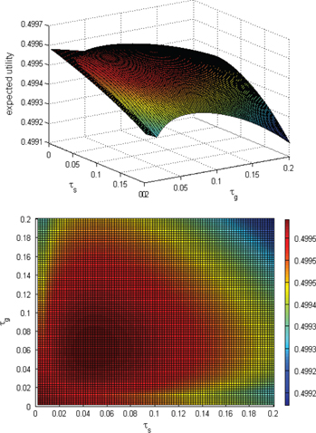
Expected utility and ECT investment.
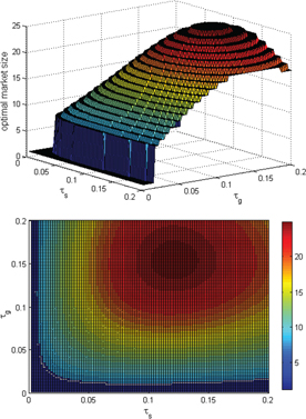
Optimal market size and ECT investment.
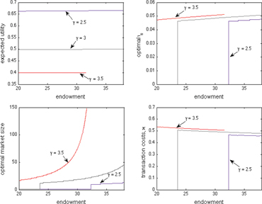
Risk aversion and endogenous exchange.
ECT calibration and endogenous exchange.
References
Acemoglu, D., P. Antràs, and E. Helpman. 2007. “Contracts and Technology Adoption.” American Economic Review 97 (3):916–43.10.1257/aer.97.3.916Search in Google Scholar
Acemoglu, D., and S. Johnson. 2005. “Unbundling Institutions.” Journal of Political Economy 113 (5):949–95.10.3386/w9934Search in Google Scholar
Allen, D. W. 2000. “Transaction Costs.” In Encylopedia of Law and Economics, edited by B. Bouckaert and G. De Geest, 893–926. Cheltenham: Edward Elgar.Search in Google Scholar
Anderlini, L., and L. Felli. 1999. “Incomplete Contracts and Complexity Costs.” Theory and Decision 46 (1):23–50.10.1023/A:1004917722235Search in Google Scholar
Antràs, P., and E. Rossi-Hansberg. 2009. “Organizations and Trade.” Annual Review of Economics 1:43–64.10.3386/w14262Search in Google Scholar
Barzel, Y. 1985. “Transaction Costs: Are They Just Costs?.” Journal of Institutional and Theoretical Economics 141:4–16.Search in Google Scholar
Besley, T., and T. Persson. 2010. “State Capacity, Conflict and Development.” Econometrica 78 (1):1–34.10.3386/w15088Search in Google Scholar
Boyd, J. H., and E. C. Prescott. 1985. “Financial Intermediary-Coalitions.” Journal of Economic Theory 38 (2):211–32.10.1016/0022-0531(86)90115-8Search in Google Scholar
Caplan, B. 2008. The Myth of the Rational Voter: Why Democracies Choose Bad Policies. Princeton, NJ: Princeton University Press.10.1515/9781400828821Search in Google Scholar
Chobanov, G., and H. Egbert. 2007. “The Rise of the Transaction Sector in the Bulgarian Economy.” Comparative Economic Studies 49:683–98.10.1057/palgrave.ces.8100226Search in Google Scholar
Coase, R. H. 1960. “The Problem of Social Cost.” Journal of Law and Economics 3:1–44.10.1086/466560Search in Google Scholar
Coase, R. H. 1992. “The Institutional Structure of Production.” American Economic Review 82 (4):713–19.Search in Google Scholar
Commission, E. 2013. “Implementing Enhanced Cooperation in the Area of Financial Transaction Tax Analysis of Policy Options and Impacts.” Commission Staff Working Document.Search in Google Scholar
De Alessi, L. 1983. “Property Rights, Transaction Costs, and X-Efficiency: An Essay in Economic Theory.” American Economic Review 73 (1):64–81.Search in Google Scholar
Dixit, A. 1996. The Making of Economic Policy: A Transaction-Cost Perspective. Cambridge, MA: MIT Press.10.7551/mitpress/4391.001.0001Search in Google Scholar
Dollery, B., and W. H. Leong. 2002. “Measuring the Transaction Sector in the Australian Economy, 1911–1991.” Australian Economic History Review 38 (3):207–31.10.1111/1467-8446.00031Search in Google Scholar
Greenwood, J., and B. Jovanovic. 1990. “Financial Development, Growth and the Distribution of Income.” Journal of Political Economy 98 (5):1076–107.10.3386/w3189Search in Google Scholar
Hart, O., and J. H. Moore. 2008. “Contracts as Reference Points.” Quarterly Journal of Economics 123 (1):1–48.10.3386/w12706Search in Google Scholar
Hazledine, T. 2001. “Measuring the New Zealand Transaction Sector, 1956–98, with an Australian Comparison.” New Zealand Economic Papers 35 (1):77–100.10.1080/00779950109544333Search in Google Scholar
Klaes, M. 2008. “The History of Transaction Costs.” In The New Palgrave Dictionary of Economics, 2nd ed. edited by S. N. Durlauf and L. E. Blume. Palgrave Macmillan. The New Palgrave Dictionary of Economics Online, Palgrave Macmillan. 27 April 2015, doi:10.1057/9780230226203.1730.Search in Google Scholar
Langlois, R. N. 2006. “The Secret Life of Mundane Transaction Costs.” Organization Studies 27:1389–410.10.1177/0170840606067769Search in Google Scholar
Levchenko, A. A. 2007. “Institutional Quality and International Trade.” Review of Economic Studies 74 (3):791–819.10.1111/j.1467-937X.2007.00435.xSearch in Google Scholar
Schumpeter, J. A. 1942. Capitalism, Socialism and Democracy. New York: Harper & Row.Search in Google Scholar
Townsend, R. M. 1978. “Intermediation with Costly Bilateral Exchange.” Review of Economic Studies 55 (3):417–25.10.2307/2297244Search in Google Scholar
Townsend, R. M. 1983. “Theories of Intermediated Structures.” Carnegie Rochester Conference Series on Public Policy 18 (Spring):221–72.10.1016/0167-2231(83)90031-3Search in Google Scholar
Townsend, R. M., and K. Ueda. 2006. “Financial Deepening, Inequality, and Growth: A Model-Based Quantitative Evaluation.” Review of Economic Studies 73 (1):251–93.10.1111/j.1467-937X.2006.00376.xSearch in Google Scholar
Wallis, J. J., and D. C. North. 1986. “Measuring the Transaction Sector in the American Economy, 1870–1970′.” In Long-Term Factors in American Economic Growth, edited by S. L. Engerman, and R. E. Gallman, 95–161. Chicago, IL: University of Chicago Press.Search in Google Scholar
Wang, N. 2003. “Measuring Transaction Costs: An Incomplete Survey.” Ronald Coase Institute, Working Paper Number 2.Search in Google Scholar
Williamson, O. E. 1979. “Transaction-Cost Economics: The Governance of Contractual Relations.” Journal of Law and Economics 22 (2):233–61.10.1086/466942Search in Google Scholar
Williamson, O. E. 1998. “Transaction Cost Economics: How It Works; Where It Is Headed.” De Economist 146 (1):23–58.10.1023/A:1003263908567Search in Google Scholar
Williamson, O. E. 2010. “Transaction Cost Economics: The Natural Progression.” American Economic Review 100:673–90.10.1257/aer.100.3.673Search in Google Scholar
Wittman, D. 1989. “Why Democracies Produce Efficient Results.” Journal of Political Economy 97 (6):1395–424.10.1086/261660Search in Google Scholar
©2015 by De Gruyter
Articles in the same Issue
- Frontmatter
- Contributions
- Aspiration Traps
- To Invite or Not to Invite a Lobby, That Is the Question
- Multi-product Bertrand Oligopoly with Exogenous and Endogenous Consumer Heterogeneity
- Directed Search with Endogenous Capacity
- Dynamic Information Revelation in Cheap Talk
- Judicial Torture as a Screening Device
- One-Sided Games in a War of Attrition
- Managerial Collusive Behavior under Asymmetric Incentive Schemes
- The Effects of Leniency on Cartel Pricing
- Transaction Costs and Institutions: Investments in Exchange
- Topics
- Patent Valuation under Spatial Point Processes with Delayed and Decreasing Jump Intensity
-
Mixed Equilibrium in a Pure Location Game: The Case of
- A Note on the Equivalence of the Conjectural Variations Solution and the Coefficient of Cooperation