What Happens When We Become Age 18? SNAP Work Requirement and SNAP Participation
-
Sungjin Lee


Abstract
This study investigates whether the Supplemental Nutrition Assistance Program (SNAP) work requirement affects SNAP participation of able-bodied adults without dependents (ABAWDs). Since 1996, ABAWDs have been required to work or participate in work programs at least 20 h per week for SNAP eligibility. Using the sample of SNAP household heads and their youngest child from administrative data for Missouri from 2004 to 2010, we compare the hazard of SNAP exit, exploiting the fact that the work requirement exemption depends on the age of the youngest child and the county of residence. Results indicate a modest reduction in SNAP participation due to the SNAP work requirement. The cumulative survival estimation indicates that the youngest child and household heads are less likely to continue to participate in SNAP for the next 24 months by 4.6 and 7.4 % points when they are expected to be subject to the work requirement.
1 Introduction
The Supplemental Nutrition Assistance Program (SNAP), formerly the Food Stamp Program, has been growing as one of the major U.S. safety net programs. In fiscal year 2023, an average of 42.1 million people per month received SNAP monthly benefits to purchase food and obtain better nutrition (Jones and Toossi 2024). Since 1996, eligibility for SNAP has been restricted for a subgroup of recipients, able-bodied adults without dependents (ABAWDs), by the Personal Responsibility and Work Opportunity Reconciliation Act (PRWORA). Under the PRWORA, ABAWDs aged at least 18 and under 50 are subject to a benefit limit of three months unless they work or participate in work programs at least 20 h per week. The work requirement was temporarily suspended nationwide in 2010 b y the American Recovery and Reinvestment Act (ARRA) due to the recession. Recently, the work requirement has been suspended nationwide again due to the COVID-19 pandemic beginning in fiscal year 2020, and has begun to reinstate the work requirement starting in July 2023.
Since 2010, legislative and administrative efforts have been made to tighten the work requirement for ABAWDs. In 2019, federal regulations were revised under an executive order to restrict conditions under which states could request the work requirement waiver and placed restrictions on states’ use of the 15 % exemption for ABAWD recipients. Also, House-passed bills in 2014 and 2018 proposed to extend the age of ABAWDs from 49 to 59 and include parents with children older than six as ABAWDs, groups formerly exempt from the rule, although the Senate rejected the proposals. A principal rationale for such proposed changes is that the work requirements promote work effort and reduce dependence on public assistance, especially for non-disabled working-age recipients.
However, there are concerns about the harm that the work requirement may cause. Some argue that ABAWDs are not work avoidants because 87 % of them were employed in the year before or after the period they received SNAP benefits (CBPP, 2018). At the same time, they suffer from job insecurity and frequent job turnover because most of them are low-skilled workers. Thus, the work requirement may deny the most vulnerable individuals access to the social safety net. Also, ABAWD rules impose massive administrative burdens on state authorities. According to the USDA audit report in 2016, states have had difficulty tracking ABAWDs for over 36 months in order to detect changes in the labor market or household activities and apply complex rules including verifying whether an individual qualifies for exemptions (e.g., through medical records) and whether they meet work requirements (e.g., by checking work hours or participation in training programs). Requiring individuals to document compliance with work requirements can increase administrative burdens for program participants and state agencies (Giannella et al. 2024).
There are relatively few studies that extensively examine the role of the work requirement on SNAP participation. In this article, we examine the impact of ABAWD rules on SNAP participation using administrative data for Missouri from 2004 to 2010. From the data, we extract SNAP household heads and their youngest children and compare the hazard of SNAP exit, employing the fact that the work requirement exemption depends on the age of children and the ABAWD rule status of the county of residence. From the results, we find a moderate negative impact of the work requirement on SNAP participation. The cumulative survival estimates indicate that children aged 18 and their household heads are less likely to continue to receive SNAP for the next 24 months by 4.6 and 7.4 % points, respectively, when they are expected to be subject to the work requirement. Also, the expected number of months of SNAP participation of children aged 18 over the next two years is reduced by 1.1 months when the county of residence imposes work requirements.
This paper contributes to the existing literature to further understand the role of the work requirement in changes in ABAWDs’ participation in SNAP. First, we can capture the impact of the work requirement rule on ABAWDs by using the age of the youngest child in a household and the variation of the work requirement across counties. Also, this research can extend our understanding regarding the response of children who encounter the work requirement rule when they become age 18, which has been rarely addressed in previous studies. Second, administrative data enables me to track the re-entry of ABAWDs in SNAP. This is important because the work requirement rule could affect the decisions of ABAWDs who return to SNAP.
2 Policy Context: SNAP Work Requirement
SNAP provides monthly benefits for eligible low-income households to ensure adequate diets. SNAP became a nationwide food assistance program in the U.S. beginning in 1974 and changed its name from the Food Stamp program in 2008. SNAP is a means-tested entitlement program that specifies that households with incomes and assets under specified levels are eligible for benefits. Unlike many other programs, few other requirements apply. As a federal program, the basic structure of SNAP benefits and eligibility is identical across the states. SNAP eligibility and benefits are based on a household, which is defined as individuals who purchase food and prepare meals together.
SNAP has been closely linked to the work requirement since the beginning of the modern SNAP in the 1970s (Mueser et al. 2019, p. 72; Botsko 2001). SNAP recipients between the ages 16 and 59 need to comply with the general work requirement by participating in SNAP Employment and Training (E&T) or workfare, and they may not voluntarily quit a job or reduce work below 30 h a week without a good reason (USDA, 2019).[1] The enactment of the Personal Responsibility and Work Opportunity Reconciliation Act (PRWORA) in 1996 put more strict work requirements on a subset of SNAP recipients, able-bodied adults without dependents (ABAWDs). Under the PRWORA, ABAWDs aged at least 18 and under 50 who are not attending secondary school are subject to a benefit limit of three months if they do not work or participate in work programs at least 80 h per month. However, ABAWDs can regain eligibility once they meet the work requirement rule during any 30-consecutive-day period. ABAWDs can be exempted from the work requirement if they are 1) responsible for as the care of a child under age 18, 2) medically certified as physically or mentally unfit for employment, 3) pregnant, or 4) already exempt from SNAP general work requirements. States may request to waive the work requirement for a certain area with an unemployment rate above 10 % or with insufficient jobs, and can exempt up to 15 % of ABAWD recipients who are not eligible for good-cause exemptions.
Aligned with the attempts to make SNAP eligibility rules more stringent, the recent SNAP policy on work requirements emphasizes economic self-sufficiency and employment of SNAP ABAWDs. In the 2018 Farm Bill, the 15 % exemption for ABAWD recipients was reduced to 12 %. Also, federal regulations were revised under Executive Order (E.O.) 13828 to restrict the work requirement waiver options of state governments in 2019. Under the new regulations, states cannot request a waiver for more than 12 months and can no longer be obtaining a state-wide work requirement waiver. Also, states are required to use the Bureau of Labor Statistics (BLS) unemployment data to prove they meet the two standard waiver conditions,[2] although other data and evidence may be accepted in exceptional circumstances.
3 Literature Review
A limited number of studies have focused on ABAWD rules and SNAP participation. Figlio et al. (2000) and Ziliak et al. (2003) are early studies that examined the relationship between the percentage of ABAWDs exempted from the work requirement and the number of SNAP beneficiaries from 1980 to 1998. Using state-level data, both studies found that increased ABAWDs with exemptions were positively associated with SNAP participation. However, both studies also indicated that ABAWD waivers had a temporary impact, and the economic situation was the dominant factor explaining SNAP participation. Mulligan (2012) and Ganong and Liebman (2018) also examined the impact of the national suspension of the SNAP work requirement due to the recession in 2009. The studies found that introducing national waivers under ARRA increased SNAP participation of ABAWDs by 2.3 and 4.1 %, respectively.
Another strand of studies used cross-sectional survey datasets, such as the American Community Survey (ACS), to evaluate the effects of SNAP work requirements, employing the age 50 cutoff as a quasi-experimental design (Stacy et al. 2018; Harris 2021; Han 2022). These studies compare outcomes between individuals just above and below age 50, leveraging the assumption that these groups are otherwise similar in observable and unobservable characteristics, absent the policy. While the evidence on labor supply responses has been mixed, reductions in SNAP participation associated with the work requirement have been consistently found. For example, Han (2022) found that exempting the requirement increased SNAP participation among ABAWDs aged 48 and 49 by 1.5 % points. Harris (2021) reported a similar effect, with estimated increases ranging from 1.5 to 1.7 % points. Stacy et al. (2018) identified a larger effect, finding an approximately 3.1 % points increase in nine states.
Studies relevant to this research are Ribar et al. (2010) and Mueser et al. (2019). Using administrative data, Ribar et al. (2010) found that adult-only households in South Carolina between 1996 and 2005 that were subject to the ABAWD rule were more likely to leave SNAP in the first five months, but the difference in exit behavior dwindled after five months. Mueser et al. (2019) extended the hazard model of Ribar et al. (2010) to two other states, Missouri and Georgia, and found similar patterns that nonelderly childless households residing in counties subject to the work requirement more likely to exit SNAP within the first six months, ranging from 2.1 to 5.6 % points. Recently, Gray et al. (2023) also found that the introduction of the work requirement reduced the rate of 18-month program retention by 23.4 % points based on the age 50 cutoff in Virginia.
This study makes two contributions to existing literature. First, it introduces a new empirical strategy that allows for estimating the effect of SNAP work requirements on a broader population segment, rather than focusing solely on individuals near the age 50 cutoff as in prior studies. Specifically, we exploit the sharp transition that occurs when the youngest child in a SNAP household turns 18, resulting in all remaining household members without qualifying exemptions subject to the ABAWD work requirement. By comparing SNAP exit probabilities at this transition point between counties that enforce the work requirement and those that do not, we estimate the average impact of the policy on SNAP participants aged 18 to 50. Second, this approach enables us to examine the policy’s effect on individuals who become adults within SNAP households, which has received limited attention in earlier research. Using administrative SNAP records, we track whether these individuals remain in their original household, exit the program, or form a new household as the head when subject to the requirement.
4 Data
4.1 Missouri SNAP Administrative Data
Our empirical analyses are based on SNAP administrative data of the State of Missouri, covering the period from January 2004 to January 2010. Missouri implemented ABAWD waivers with a lenient definition of labor surplus and a 15 % exemption for small population counties from 2001 (Mueser et al. 2019). Also, non-compliant ABAWDs may receive SNAP benefits for three months. As a result, the number of counties with exemptions or waivers constantly grew to 105 out of 115 areas in 2006 from 27 in 2001. However, Missouri started applying a strict three-month limit to all ABAWDs and reduced the use of exemptions in January 2007. The number of counties with waivers fell sharply in the following years until January 2009. After the enactment of ARRA due to the recession, all 115 areas (114 counties and Saint Louis city) were exempted from February 2009. The variation of ABAWD waiver status in counties allows us to distinguish whether ABAWDs face the work requirement depending on the date and the county of residence (Figure 1).

Counties in Missouri that exempted or waived from the work requirement. Note: The number of counties exempted or waived from the work requirement is recorded as of January for each year between 2004 and 2010. The State of Missouri comprises 115 jurisdictions—114 counties and the independent city of St. Louis. The numbers are obtained from the Missouri Department of Social Service (Accessed May 2025) and Mueser et al. (2019) p.73.
The administrative data of Missouri contains detailed monthly information on SNAP households. The data are organized around a household head and household members. A household head is a person who establishes a SNAP household, and the period of SNAP certification of a household head applies to all household members. All SNAP recipients have two identifiers in the data: household and individual identifiers. The household identifier is assigned to SNAP recipients in the same household so that we can identify household members. Also, each recipient has a unique individual identifier, which enables us to create longitudinal data for 73 months by matching individual identifiers. Since the individual identifier does not change once it is assigned, we can track when recipients leave or re-enter SNAP, move between households, or become a new household head. The data provides the demographic information of all recipients, including gender, date of birth, race, and county of residence. Also, the data includes start and end dates of benefit periods, status in SNAP, amount of benefits, and participation in other welfare programs. However, the data do not contain reliable indicators, including disability and school enrollment, which can serve as the basis to be exempted from the work requirement rule. Also, we cannot identify the status of employment from the data.
For the main analysis regarding monthly participation, we use the status indicator of individuals to determine their SNAP participation. We define individuals as SNAP participants who were assigned an ‘active’ status in a given month. For individuals with the status of ‘closed’, ‘applying’, or ‘expired’, or where there is no record for the month, we define them as inactive in a given month. SNAP recipients with two consecutive inactive statuses, or for whom the record is missing, are considered to have exited from SNAP. To smooth the data, one month missing between active months is considered as an active status. This smoothing process can eliminate artificial SNAP exit related to administrative “churning,” which does not indicate actual changes in participation or income (Ribar et al. 2010).
We supplement the two datasets based on the household’s county of residence. As a primary policy measure, the ABAWD waiver status of the county of residence is matched to each SNAP recipient. Also, the monthly unemployment rate of counties from the Local Area Unemployment Statistics (LAUS) is employed as an indicator of the health of the local economy.
4.2 Sample Selection
The complete SNAP data for Missouri from Jan 2004 to Jan 2010 (73 months) includes records for 9,98,377 households with 2.1 million unique individuals. From the data, our primary focus is on SNAP household heads and their youngest children[3] aged between 16 and 20. I extract household heads and the youngest children who are both active SNAP recipients from each month. To measure the hazard of exiting SNAP next month, active months less than three months before January 2010 are omitted. We also exclude records showing changes to the date of birth, households without information on household heads, absence of individual or household identifiers, or missing information on the amount of SNAP benefit. The baseline sample contains 57,960 unique household heads and 60,540 children. One of the limitations in our data is that we cannot identify information such as medical conditions or full-time student status of each individual, which are valid reasons for the work requirement exemption when they are expected to be subject to the requirement.
We calculate the ages on a monthly basis (based on the date of birth and time to the middle of the month), so we obtain 60 age groups by age of the youngest child between 16 and 20. As shown in Figure 2, we construct risk sets based on the age groups and divide them by the ABAWD rule status in the county of residence. Thus, we obtain four groups: 1) the youngest children and 2) their household heads in exempt counties; 3) the youngest children and 4) household heads in nonexempt counties. Observations in each risk set include duplicate heads and children who have multiple spells or participated in SNAP for more than one month. Also, individuals with multiple SNAP receipt months may be classified by different ABAWD work rule statuses in risk sets at different points since the ABAWD rule status in the county of residence can change over time, or individuals may move between counties. We assume that each risk set is independent of the other risk sets. In the unusual case of a head who has multiple youngest children at a given point in time, there are duplicate observations of heads as youngest children. For example, a record of a mother with 18-year-old twins is shown twice in the risk set of heads for age 18.
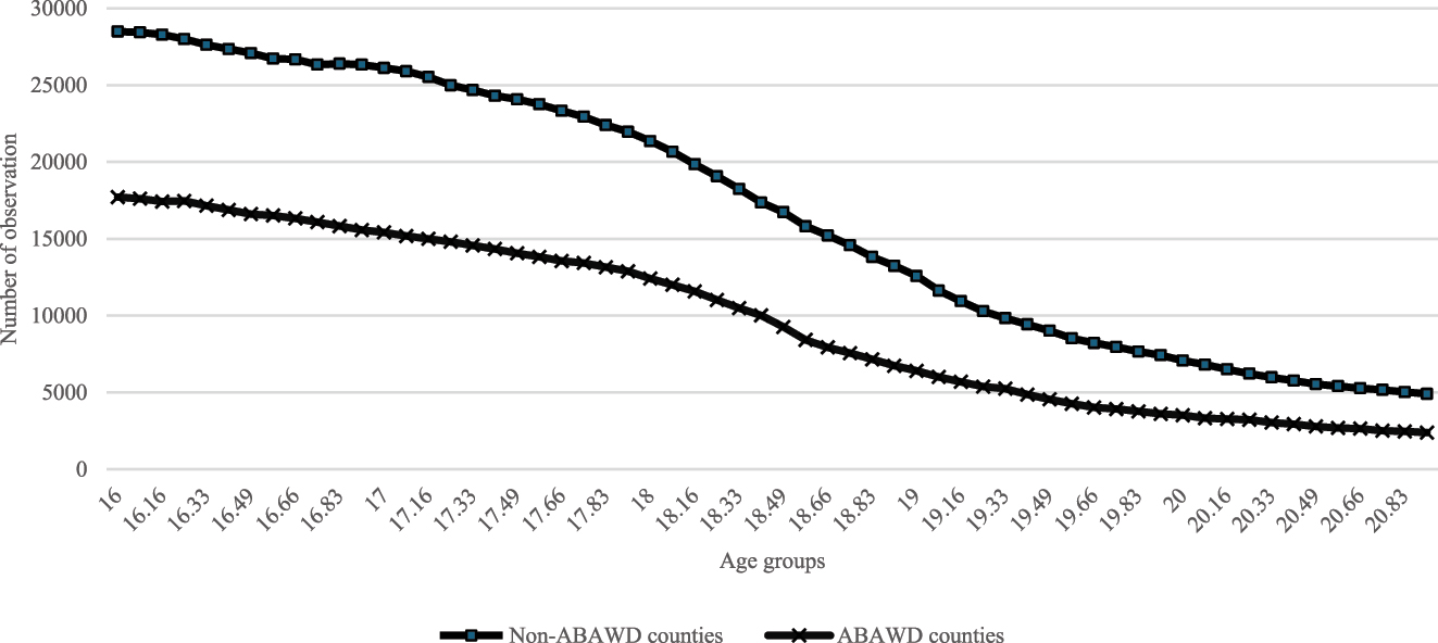
Number of observations by the age of youngest child and residence. Note: Sixty age groups are constructed on a monthly basis, calculated using the date of birth and the midpoint of each month based on the age of the youngest child between 16 and 20, using Missouri SNAP administrative data from January 2004 to January 2010. Each age group includes the youngest child and their household head and is divided by the work requirement status of their county of residence.
The total observations include 792,826 observations of heads and 792,826 observations of children from all 60 age groups. The number of observations in exempt counties is always higher than in nonexempt counties. However, the number of observations decreases from age 16 and falls sharply after age 18 in both nonexempt and exempt counties. This common trend could be related to children’s legal independence from their parents when they reach the age of 18.
We select another sample to examine the relationship between SNAP benefit months and ABAWD rules. The second sample includes all children who have an 18th birthday as active SNAP recipients, and their household heads. Those children are not limited to being the youngest child but include all active SNAP recipients at age 18. We track their SNAP records for the following two years after age 18 to examine the difference in SNAP participation between exempt and nonexempt counties. Thus, the active spells of duration less than 24 months before January 2010 are omitted. The sample includes 36,409 unique children. As a placebo, children who have turned age 16 are selected in parallel analyses of ABAWD rules. We obtain 50,650 unique children aged 16.
Table 1 displays descriptive statistics for the sample, including children at age 18 and 16 who receive SNAP benefits in the data. Demographic characteristics are based on the month at age 18 and 16, respectively. For children aged 18, 43 % of children live in nonexempt counties, and 48 % of them are female. More than half of the children (55 %) are classified as White, and 42 % of them are African American. The average number of household members is about four individuals, and 30 % of children are the youngest child in the household. About 13 % of children are from households with dependents under age 18 who are not children of the household heads (e.g., a nephew). Also, 13 % of children are from households that participate in other welfare programs. The distribution of calendar year is relatively even from 2004 to 2007; for the year 2008, I include only two months (January and February). As shown in Table 1, the major characteristics of children aged 16 are similar to those of children aged 18.
Sample descriptive statistics for children aged exactly 18 and 16.
| Children age 18 | Children age 16 | |||||||
|---|---|---|---|---|---|---|---|---|
| Mean | SD | Min | Max | Mean | SD | Min | Max | |
| Residence in nonexempt counties | 0.43 | 0.50 | 0 | 1 | 0.44 | 0.50 | 0 | 1 |
| Female | 0.48 | 0.50 | 0 | 1 | 0.50 | 0.50 | 0 | 1 |
| Age of household head | 41.86 | 5.82 | 19.5 | 82 | 39.77 | 5.80 | 18.58 | 79.59 |
| White | 0.55 | 0.50 | 0 | 1 | 0.57 | 0.50 | 0 | 1 |
| Black | 0.42 | 0.49 | 0 | 1 | 0.40 | 0.49 | 0 | 1 |
| Other* | 0.04 | 0.19 | 0 | 1 | 0.03 | 0.18 | 0 | 1 |
| Number of household members | 4.09 | 1.73 | 2 | 19 | 4.24 | 1.69 | 2 | 19 |
| Presence of dependents under age 18 other than children | 0.13 | 0.33 | 0 | 1 | 0.08 | 0.27 | 0 | 1 |
| Participation in other welfare programs | 0.13 | 0.34 | 0 | 1 | 0.13 | 0.34 | 0 | 1 |
| Youngest child | 0.30 | 0.46 | 0 | 1 | 0.30 | 0.46 | 0 | 1 |
| SNAP benefit | 328.55 | 185.47 | 0 | 1682 | 340.05 | 187.91 | 0 | 1707 |
| Calendar year 2004 | 0.22 | 0.42 | 0 | 1 | 0.23 | 0.42 | 0 | 1 |
| Calendar year 2005 | 0.24 | 0.42 | 0 | 1 | 0.24 | 0.43 | 0 | 1 |
| Calendar year 2006 | 0.24 | 0.43 | 0 | 1 | 0.25 | 0.43 | 0 | 1 |
| Calendar year 2007 | 0.25 | 0.43 | 0 | 1 | 0.25 | 0.43 | 0 | 1 |
| Calendar year 2008 | 0.05 | 0.21 | 0 | 1 | 0.04 | 0.20 | 0 | 1 |
| Total number | 36,409 | 50,650 | ||||||
-
This table presents descriptive statistics for active SNAP households with children aged 16 and 18, based on Missouri administrative data from January 2004 to January 2010. Other race categories include Asian, Hispanic, American Indian, and Native Pacific Islander.
5 Empirical Strategy
5.1 Hazard Model
The main approach is to estimate hazard models to examine the impact of SNAP work requirements on the risk of exit from SNAP, taking into account the age of the youngest child and the county of residence. Specifically, we estimate the discrete-time hazard of exit for children and household heads in 60 age groups using a linear probability model. By the definition of the work requirement, household heads and children under age 18 are exempted from the ABAWD rule regardless of residence. Once the youngest child reaches age 18, however, both the head and child are subject to the ABAWD rule if they live in a nonexempt county and do not qualify for an individual exemption. Thus, we expect the chance of leaving SNAP for individuals in age groups over age 18, especially for the three months after age 18, will differ by the ABAWD status of the county of residence if the work requirement affects SNAP participation.
For a participant i, the probability of exiting SNAP in the next month (defined as inactive status for the next two consecutive months) at a given child age at time t and in county c is specified as:
where λ
ict
is the probability of exiting SNAP in the next month t+1 (Y
i,t+1=0) given participation on month t (Y
it
=1). The vector X
ct
includes the unemployment rate and the squared unemployment rate in county c in time t. Also, the vector Z
it
includes race, gender, amount of SNAP benefits, number of household members, and an indicator for participation in other welfare programs for an individual i at time t.
Based on estimates of coefficients from equation (1), we calculate the predicted hazard of each age group with the average unemployment rate, amount of benefits, and the number of household members for all individuals in the sample in county c in month t. More specifically, the prediction model is defined as:
where
5.2 OLS Model
The second approach is to examine the impact of the work requirement on SNAP participation over a longer period. Unlike the first approach, estimating risks of leaving SNAP in the next month, we track records of SNAP receipt of children aged 16, aged 18, and their household heads for the next two years. The work requirement rule could affect the decisions of SNAP leavers to rejoin the program if they are subject to the rule. Our specification of the model for individual i is:
where M i is the total number of months of SNAP receipt for an individual i in the following 23 months. In the model, we control the average value of unemployment and the ABAWD status of county c, where the initial residence of individual i for the following 23 months. The average unemployment rate and the squared unemployment rate in county c capture economic opportunities. Also, the main interest is the proportion of months that county c is subject to the work requirement rule (varying from 0 to 1). Also, the model includes year fixed effects (ϕ t ), regional fixed effects (η r ), and the vector of individual characteristics (Z i ) including race, gender, amount of SNAP benefits, number of household members, and an indicator for participation in other welfare programs at exact ages 18 and 16. All standard errors are clustered at the county level.
6 Main Results
6.1 Hazard Model
6.1.1 Descriptive Analysis
In Figures 3 and 4, we plot Kaplan-Meier estimates of the hazard of SNAP exit in each month for children and household heads. Figure 3 presents unconditional SNAP exit probability by SNAP duration by the number of months in SNAP for children and household heads who have an identified spell start date. There are two features to be noted. First, SNAP exit probabilities dwindled with SNAP duration, suggesting negative duration dependence. In other words, individuals with a longer period of SNAP are less likely to leave SNAP in the next month. Second, we observe the higher exit probability every 6-month interval, which indicates the impact of the recertification process on SNAP exit, aligned with the findings of the previous literature.
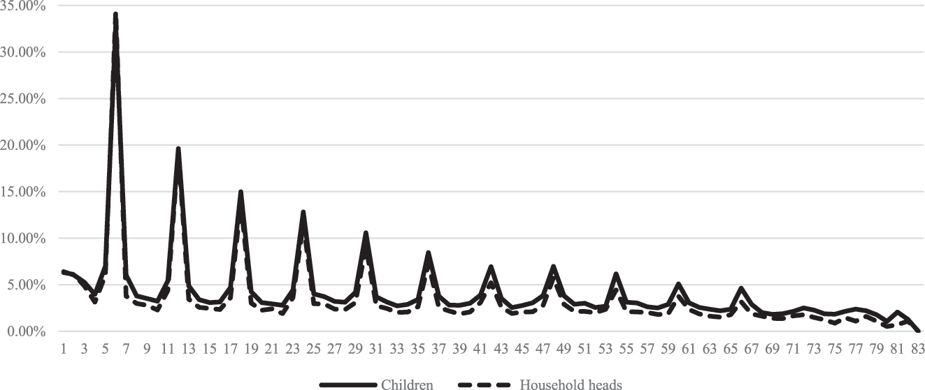
Unconditional SNAP exit probabilities by SNAP duration. Note:This table presents selected discrete-time estimates from Equation (1) for children aged 16–20 years and 11 months, and their household heads who participated in SNAP in Missouri between January 2004 and November 2010. Each column corresponds to a separate specification for a specific subgroup. The main sample represents children and household heads without other dependents under age 18 in the household, and with household heads younger than 49. Year and region fixed effects are included, and standard errors are clustered at the county level. Standard errors are in parentheses. For brevity’s sake, standard errors for dummies are not shown in the table. *Significant at 0.1 level. **significant at 0.05 level. ***significant at 0.01 level.
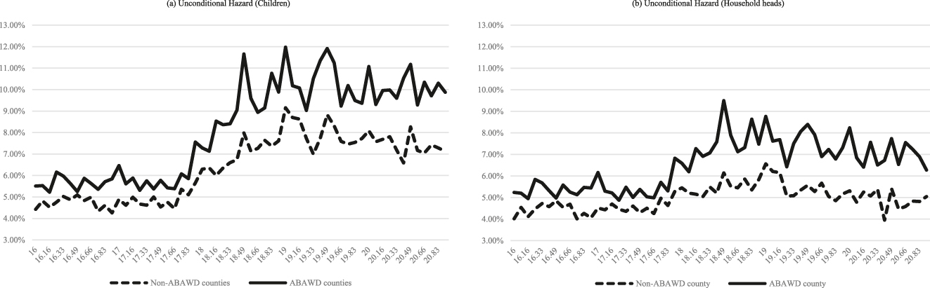
Unconditional Hazard analysis of children and household heads by the age of children and county in residence. Note:This figure presents the unconditional hazard of SNAP exit across 60 age groups, defined for children aged 16–20 years and 11 months, and their household heads who participated in SNAP in Missouri between January 2004 and November 2010. Each age group is divided by the SNAP work requirement status in the household’s county of residence at the time.
Figure 4 shows the unconditional hazard of SNAP exit ((a) and (b)) by the work requirement status of the county for children and household heads. From the unconditional hazard of SNAP exit ((a) and (b)) in Figure 4, three features need to be noted. First, the chance of leaving SNAP is higher for all age groups of children and household heads who live in nonexempt counties than those who live in exempt counties. Aligned with the previous literature regarding the relationship between the economy and SNAP participation, higher exit probabilities in nonexempt counties reflect their lower unemployment rates or better economic conditions. Second, the exit probabilities of children and household heads start to increase sharply at child age 18, regardless of county of residence, although the hazards of SNAP exit for household heads are lower than those of children for any given age of children. One of the possible explanations is the independence of children. In Missouri, children become legally majority at the age of 18 so that they may separate from parental households and establish independent households. In this case, the incentive of household heads to stay in SNAP is reduced due to a lower net income threshold and SNAP benefits as the number of household members declines, given that SNAP benefits are determined by household size and net gross income. Lastly, the difference in SNAP exit probabilities between exempt and nonexempt counties increases after age 18 for both children and household heads.
6.1.2 Multivariate Analysis
Table 2 presents selected coefficient estimates from the discrete-time hazard model based on equation (1). Interaction terms between the ABAWDs rule status and the ages of children,
Discrete-time hazard of SNAP exit of children and household heads.
| Children | Household heads | |||||||
|---|---|---|---|---|---|---|---|---|
| Main sample | Full | Main sample | Full | |||||
| (1) | (2) | (3) | (4) | |||||
| Interaction of ABAWDs tule in the county of residence with age dummies | ||||||||
| Age 16 and 1 month | −0.0055 | −0.0040 | −0.0074 | −0.0060 | ||||
| Age 16 and 2 months | −0.0028 | −0.0041 | −0.0033 | −0.0040 | ||||
| Age 16 and 3 months | 0.0060 | 0.0030 | 0.0056 | 0.0013 | ||||
| Age 16 and 4 months | 0.0022 | −0.0016 | −0.0003 | −0.0028 | ||||
| Age 16 and 5 months | −0.0015 | −0.0035 | −0.0028 | −0.0050 | ||||
| Age 16 and 6 months | −0.0100 | * | −0.0094 | ** | −0.0106 | ** | −0.0111 | ** |
| Age 16 and 7 months | −0.0019 | −0.0001 | −0.0035 | −0.0015 | ||||
| Age 16 and 8 months | −0.0032 | −0.0042 | −0.0048 | −0.0063 | ||||
| Age 16 and 9 months | 0.0027 | −0.0004 | 0.0019 | −0.0007 | ||||
| Age 16 and 10 months | 0.0015 | 0.0003 | 0.0005 | 0.0001 | ||||
| Age 16 and 11 months | 0.0036 | 0.0049 | 0.0001 | 0.0016 | ||||
| Age 17 | 0.0081 | 0.0047 | 0.0069 | 0.0040 | ||||
| Age 17 and 1 month | 0.0031 | −0.0010 | 0.0019 | −0.0037 | ||||
| Age 17 and 2 months | 0.0021 | −0.0021 | −0.0044 | −0.0071 | ||||
| Age 17 and 3 months | −0.0074 | −0.0048 | −0.0096 | * | −0.0083 | * | ||
| Age 17 and 4 months | −0.00001 | 0.0003 | −0.0026 | −0.0013 | ||||
| Age 17 and 5 months | −0.0044 | −0.0073 | −0.0060 | −0.0084 | * | |||
| Age 17 and 6 months | 0.0026 | 0.0009 | −0.0009 | −0.0021 | ||||
| Age 17 and 7 months | 0.0010 | −0.0048 | −0.0028 | −0.0076 | * | |||
| Age 17 and 8 months | −0.0019 | −0.0022 | −0.0064 | −0.0056 | ||||
| Age 17 and 9 months | −0.0035 | −0.0045 | −0.0064 | −0.0057 | ||||
| Age 17 and 10 months | −0.0036 | −0.0041 | −0.0049 | −0.0062 | ||||
| Age 17 and 11 months | 0.0124 | ** | 0.0079 | 0.0064 | 0.0028 | |||
| Age 18 | 0.0016 | −0.0007 | −0.0002 | −0.0007 | ||||
| Age 18 and 1 month | 0.0001 | −0.0031 | 0.0003 | −0.0023 | ||||
| Age 18 and 2 months | 0.0206 | *** | 0.0143 | *** | 0.0176 | *** | 0.0087 | * |
| Age 18 and 3 months | 0.0181 | *** | 0.0090 | * | 0.0139 | ** | 0.0061 | |
| Age 18 and 4 months | 0.0126 | * | 0.0068 | 0.0056 | 0.0031 | |||
| Age 18 and 5 months | 0.0163 | ** | 0.0115 | ** | 0.0153 | ** | 0.0108 | ** |
| Age 18 and 6 months | 0.0297 | *** | 0.0250 | *** | 0.0256 | *** | 0.0203 | *** |
| Age 18 and 7 months | 0.0190 | *** | 0.0119 | ** | 0.0178 | *** | 0.0093 | * |
| Age 18 and 8 months | 0.0020 | 0.0039 | 0.0084 | 0.0023 | ||||
| Age 18 and 9 months | 0.0040 | 0.0019 | 0.0044 | −0.0001 | ||||
| Age 18 and 10 months | 0.0334 | *** | 0.0208 | *** | 0.0303 | *** | 0.0181 | *** |
| Age 18 and 11 months | 0.0057 | 0.0090 | 0.0046 | 0.0012 | ||||
| Age 19 | 0.0272 | *** | 0.0141 | ** | 0.0216 | *** | 0.0063 | |
| Age 19 and 1 month | 0.0036 | 0.0003 | 0.0013 | −0.0020 | ||||
| Age 19 and 2 months | 0.0002 | 0.0001 | −0.0008 | −0.0006 | ||||
(continued)
| Children | Household heads | |||||||
|---|---|---|---|---|---|---|---|---|
| Main sample | Full | Main sample | Full | |||||
| (1) | (2) | (3) | (4) | |||||
| Interaction of ABAWDs tule in the county of residence with age dummies | ||||||||
| Age 19 and 3 months | 0.0096 | −0.0014 | 0.0108 | −0.0023 | ||||
| Age 19 and 4 months | 0.0313 | *** | 0.0212 | *** | 0.0171 | ** | 0.0086 | |
| Age 19 and 5 months | 0.0204 | ** | 0.0220 | *** | 0.0165 | * | 0.0115 | * |
| Age 19 and 6 months | 0.0227 | ** | 0.0165 | ** | 0.0155 | * | 0.0123 | * |
| Age 19 and 7 months | 0.0226 | ** | 0.0149 | ** | 0.0182 | ** | 0.0103 | |
| Age 19 and 8 months | 0.0073 | 0.0024 | 0.0044 | −0.0034 | ||||
| Age 19 and 9 months | 0.0125 | 0.0128 | * | 0.0120 | 0.0057 | |||
| Age 19 and 10 months | 0.0177 | * | 0.0048 | 0.0133 | 0.0029 | |||
| Age 19 and 11 months | 0.0108 | 0.0016 | 0.0131 | 0.0051 | ||||
| Age 20 | 0.0371 | *** | 0.0150 | * | 0.0260 | ** | 0.0127 | * |
| Age 20 and 1 month | 0.0214 | * | 0.0023 | 0.0251 | ** | 0.0041 | ||
| Age 20 and 2 months | 0.0049 | 0.0072 | −0.0058 | −0.0054 | ||||
| Age 20 and 3 months | 0.0011 | 0.0064 | −0.0008 | 0.0079 | ||||
| Age 20 and 4 months | 0.0177 | 0.0085 | 0.0062 | −0.0059 | ||||
| Age 20 and 5 months | 0.0297 | ** | 0.0244 | *** | 0.0067 | 0.0110 | ||
| Age 20 and 6 months | 0.0279 | ** | 0.0139 | 0.0204 | * | 0.0064 | ||
| Age 20 and 7 months | 0.0241 | * | 0.0059 | 0.0151 | 0.0037 | |||
| Age 20 and 8 months | 0.0332 | *** | 0.0181 | ** | 0.0307 | ** | 0.0132 | |
| Age 20 and 9 months | 0.0049 | 0.0079 | 0.00003 | 0.0074 | ||||
| Age 20 and 10 months | 0.0187 | 0.0153 | * | 0.0015 | 0.0046 | |||
| Age 20 and 11 months | 0.0354 | ** | 0.0126 | 0.0117 | −0.0042 | |||
| Year fixed effects | x | x | x | x | ||||
| Regional fixed effects | x | x | x | x | ||||
| SNAP duration | ||||||||
| Observation | 523523 | 792826 | 523523 | 792826 | ||||
| Adjusted R-squared | 0.0123 | 0.0115 | 0.0097 | 0.0091 | ||||
-
This table presents selected discrete-time estimates from Equation (1) for children aged 16–20 years and 11 months, and their household heads who participated in SNAP in Missouri between January 2004 and November 2010. Each column corresponds to a separate specification for a specific subgroup. The main sample represents children and household heads without other dependents under age 18 in the household, and with household heads younger than 49. Year and region fixed effects are included, and standard errors are clustered at the county level. Standard errors are in parentheses. For brevity’s sake, standard errors are not shown in the table. *Significant at 0.1 level. **Significant at 0.05 level. ***Significant at 0.01 level.
In Columns 2 and 4, we examine the full sample of children and household heads without considering the age of the household head. From Column 2 for children and Column 4 for household heads, the results have similar patterns to those in Columns 1 and 3, but show fewer significant estimates and generally smaller magnitudes of coefficients, which support our main finding that the difference in SNAP exit probability is associated with the work requirement.
One of the potential concerns is that standard errors of estimates may correlate with each other since the data contains duplicate individuals and many individuals in each county. To address this, we estimate cluster-robust standard errors at both the individual and county levels for equation (1) and find that the results remain unchanged. We also test the model using county fixed effects in place of regional fixed effects and again find that the findings are consistent.
We cannot directly compare the magnitude of estimates of interaction terms from the main and full sample, since confining the new sample also changes estimates of age dummies in exempt counties. Also, it is hard to assess the overall impact of the work requirement on SNAP exit due to fluctuations in exit probabilities by the age of children. Thus, we plot the predicted exit probabilities with the average unemployment rate, the amount of benefits, and the number of household members using equation (2) based on estimates in Table 2. In Figure 5, the left-side figures ((a) and (c)) are the predicted SNAP exit probabilities for children and household heads based on the full sample, and the right-side figure is for the main sample. As shown in Table 2, we cannot observe a significant difference in SNAP exit probabilities for children aged 16 and 17 in the figures. Figures (b) and (d) indicate that children and household heads in the main sample have a higher chance of leaving SNAP after age 18 for both exempt and nonexempt counties compared to the full sample. This may be partly because households with younger household heads and no other dependents may be more likely to find jobs or because they are less likely to meet income thresholds. However, in households with children over age 18, household heads and children in nonexempt counties still show a higher chance of leaving SNAP compared to those in exempt counties and also those in nonexempt counties from the full sample.
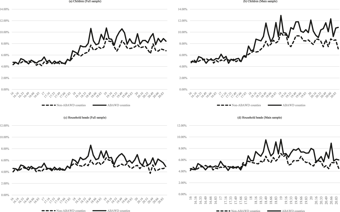
Predicted SNAP exit probabilities of children and household heads by the age of child and the county of residence. Note:This figure presents the predicted hazard of SNAP exit across 60 age groups, defined for children aged 16–20 years and 11 months, and their household heads who participated in SNAP in Missouri between January 2004 and November 2010. Based on estimates of coefficient from equation (1), the predicted hazard of each age group is calculated with the average unemployment rate, amount of SNAP benefits, and the number of household members for all individuals in the sample (equation (2)). Each age group is divided by the SNAP work requirement status in the household’s county of residence at the time.
Figure 6 displays the cumulative survival function estimates for the full and main samples based on the predicted hazard rate of each age group. For example, the predicted SNAP exit rate in ABAWD counties is 5.17 % at age 16 and 5.13 % at age 16 and 1 month. This corresponds to survival rates of 94.83 % and 94.87 %, respectively. The cumulative survival rate is calculated by multiplying two survival rates, 89.96 % at age 16 and 1 month. For survival analysis, we divide the sample into two groups of children and household heads by the age of children: 1) children aged 16 to 17 and 11 months, and 2) children aged 18 to 20 and 11 months, and by their ABAWD rule status of the county of residence. Thus, this analysis presents the overall impact of the work requirement for the two age groups. For the full sample ((a) and (c)), children aged 18 to 20 and 11 months in nonexempt counties have a lower chance of staying on SNAP by about 4.8 % points than children in exempt counties. Also, household heads with children aged 18 to 20 and 11 months in nonexempt counties are less likely to stay on SNAP by 6.7 % points compared to heads in exempt counties. In the case of age 16 to 17 and 11 months, the difference is less than 2 % for both children and household heads. For household heads and children in the main sample, the results indicate higher exit probabilities of household heads in nonexempt counties compared to those from the full sample. Household heads and children aged 18 to 20 and 11 months in nonexempt counties have 7.4 and 4.6 % points lower chances of staying on SNAP, respectively.
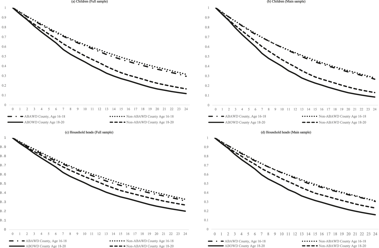
Survival analysis of children and household heads by age of children and county in residence based on predicted exit probabilities. Note:This figure presents the cumulative survival rates for children and household heads based on the predicted hazard of SNAP exit estimated from Equation (2). Survival rates are calculated separately for two age groups—children aged 16–17 years and 11 months, and those aged 18–20 years and 11 months—and are further disaggregated by the SNAP work requirement status in the household’s county of residence at the time.
6.2 OLS Model
In Table 3, we examine the relationship between the work requirement and SNAP participation for 24 months based on equation (3). We measure the number of months of participation in two ways. In Panel A, we count the months of SNAP receipts for children who are dependents under the same household head. In Panel B, we extend the definition of SNAP participation to receipt of SNAP by children, including those in other households or who establish independent SNAP households. If the work requirement increases the chance of leaving SNAP as shown in the previous section, we expect the ABAWD rule will also affect the decision of individuals to return to SNAP.
SNAP participation of children age 16 and 18 for subsequent 24 months by ABAWD rule in county of residence.
| Children age 18 | Children age 16 | |||||||
|---|---|---|---|---|---|---|---|---|
| Group B | All | Group B | All | |||||
| (1) | (2) | (3) | (4) | |||||
| A: Given status | ||||||||
| Avg. ABAWD | −0.65 | ** | 0.22 | * | 0.31 | 0.11 | ||
| (0.28) | (0.12) | (0.23) | (0.10) | |||||
| Avg. Unemployment rate | 0.51 | 0.59 | *** | 1.06 | ** | 0.80 | *** | |
| (0.50) | (0.21) | (0.42) | (0.19) | |||||
| Avg. squared unemployment rate | 0.001 | 0.002 | −0.04 | −0.03 | * | |||
| (0.04) | (0.02) | (0.03) | (0.01) | |||||
| Demographic controls | X | X | X | X | ||||
| Observation | 6,435 | 36,409 | 10,745 | 50,650 | ||||
| B: Any status | ||||||||
| Avg. ABAWD | −1.10 | *** | −0.20 | * | −0.18 | −0.13 | ||
| (0.28) | (0.12) | (0.23) | (0.10) | |||||
| Avg. Unemployment rate | −0.20 | 0.53 | ** | 0.49 | 0.58 | *** | ||
| (0.50) | (0.21) | (0.40) | (0.18) | |||||
| Avg. squared unemployment rate | 0.06 | 0.01 | −0.003 | −0.01 | ||||
| (0.04) | (0.02) | (0.03) | (0.01) | |||||
| Demographic controls | X | X | X | X | ||||
| Observation | 6,435 | 36,409 | 10,745 | 50,650 | ||||
-
This table presents selected OLS estimates from Equation (3) for children who participated in SNAP at the exact ages of 16 and 18 between January 2004 and January 2010. Each column corresponds to a separate specification for a specific subgroup. Group B restricts the sample to children in households without other dependents under age 18 and with household heads younger than 47. In Panel A, SNAP participation is measured by the number of months children received benefits as dependents in the same household. In Panel B, SNAP participation includes benefit receipt by children regardless of household composition, including cases where they are in different households or have formed independent SNAP households. Year and region fixed effects are included, and standard errors are clustered at the county level and reported in parentheses. *Significant at 0.1 level. **Significant at 0.05 level. ***Significant at 0.01 level.
The baseline sample is composed of children who participate in SNAP at the exact age of 18. We extract a sub-sample, Group B, which includes children in households without other dependents under age 18 and where the household head is under 47. Similar to the main sample in the previous section, Group B is a group of children who are more likely to be subject to the work requirement. As a placebo, we select children aged 16 and Group B from them using the same definition.
In column 1 of Panel A in Table 3, there is a negative and significant effect on SNAP receipt for each month (out of 24) the child’s initial county is subject to the work requirement beginning at age 18. After controlling for the average unemployment rates and demographic characteristics, SNAP participation of children is reduced by 0.65 months for a county that is subject to the work requirement in comparison to one that is not. For all children aged 18, the effect is positive but relatively small and marginally significant at the 10 % level. When we extend the definition of participation in Panel B, the magnitude of the effect is larger and shows the expected negative direction. The results indicate that the county ABAWD rule leads to a decrease in participation of Group B by 1.1 months. We find a negative effect for the sample with all children, but the magnitude is small (0.2 months) and marginally significant. For children aged 16, we do not find any significant impact of the ABAWD rule in the county on SNAP participation as expected.
In Table 4, we estimate the same model for household heads. We select household heads who have a youngest child aged 16 and 18, respectively. Similar to the results for children, we do not find a meaningful effect on SNAP participation for household heads with children aged 16 in Panels A and B. For household heads with children aged 18 in Panel A, SNAP participation of heads in Group B decreases by 1.12 months when their county of residence imposes a work requirement. For all household heads with children aged 18, their participation in SNAP also decreased by 0.91 months due to the work requirement. The difference in estimates between Group B and the full sample is not as large as that of children since the majority of heads in the full sample belong to Group B. Interestingly, I find that the results in Panel A and B show a similar effect of the work requirement on participation for household heads with children aged 18. As expected, in contrast to the case of children, the results indicate that household heads are very unlikely to return to SNAP in another household. In sum, we take the results above as evidence of the negative impact of the work requirement on SNAP participation. The work requirement increases the chance of leaving SNAP and decreases the probability of re-entering SNAP for children and household heads likely to face the work requirement.
SNAP participation of household heads with children age 16 and 18 for subsequent 24 months by ABAWD rule in county of residence.
| Household heads | Household heads | ||||||
|---|---|---|---|---|---|---|---|
| with the youngest | with the youngest | ||||||
| child age 18 | child age 16 | ||||||
| Group B | All | Group B | All | ||||
| (1) | (2) | (3) | (4) | ||||
| A: Given status | |||||||
| Avg. ABAWD | −1.12 | *** | −0.72 | *** | 0.11 | −0.13 | |
| (0.31) | (0.24) | (0.23) | (0.19) | ||||
| Avg. Unemployment rate | −0.23 | −0.25 | 0.80 | ** | 0.49 | ||
| (0.55) | (0.43) | (0.41) | (0.34) | ||||
| Avg. squared unemployment rate | 0.067 | 0.07 | ** | −0.02 | −0.0004 | ||
| (0.04) | (0.03) | (0.03) | (0.03) | ||||
| Demographic controls | X | X | X | X | |||
| Observation | 6,326 | 10,815 | 10,547 | 15,151 | |||
| B: Any status | |||||||
| Avg. ABAWD | −1.13 | *** | −0.74 | *** | 0.04 | −0.17 | |
| (0.30) | (0.24) | (0.23) | (0.19) | ||||
| Avg. Unemployment rate | −0.22 | −0.20 | 0.75 | * | 0.51 | ||
| (0.54) | (0.42) | (0.40) | (0.34) | ||||
| Avg. squared unemployment rate | 0.07 | 0.06 | ** | −0.017 | −0.001 | ||
| (0.04) | (0.03) | (0.03) | (0.03) | ||||
| Demographic controls | X | X | X | X | |||
| Observation | 6,326 | 10,815 | 10,547 | 15,151 | |||
-
This table presents selected OLS estimates from Equation (3) for household heads who participated in SNAP with a child aged 16 or 18 between January 2004 and January 2010. Each column corresponds to a separate specification for a specific subgroup. Group B restricts the sample to household heads under age 47 and without any other dependents under 18. In Panel A, SNAP participation is measured by the number of months household heads received benefits while residing in the same household. In Panel B, the definition of SNAP participation is extended to include benefit receipt by household heads regardless of household composition, including cases where they reside in different households or have established independent SNAP households. Year and region fixed effects are included, and standard errors are clustered at the county level and reported in parentheses. *Significant at 0.1 level. **Significant at 0.05 level. ***Significant at 0.01 level.
7 Conclusions
In this study, we examine the impact of the work requirement on SNAP participation, taking into account variations of the county of residence by the ABAWD rule imposition and the ages of children. The results reported in this study are intended to treat the effect of the work requirement since the data do not allow us to distinguish whether particular individuals face the requirement. However, there may be a potential endogeneity issue if we incorporate the actual ABAWD status of individuals into the model. The SNAP regulation of Missouri indicates that SNAP recipients may report changes in their situations to be exempted from the requirement, such as temporary disability. Thus, it is reasonable to assume that the work requirement may change the behaviors of individuals subject to the rule.
Based on Missouri’s administrative data from 2004 to 2010, our findings suggest a modest negative effect of the work requirement on SNAP participation for individuals likely to be subject to the rule. The cumulative survival estimates from the discrete hazard of SNAP exit show that children aged 18 to 20 and their household heads in nonexempt counties have a 4.6 and 7.4 % points higher chance of leaving SNAP, respectively, compared to those in exempt counties. We do not find a meaningful difference in SNAP exit behaviors of children and household heads when a child is under age 18. Given that SNAP households with a minority dependent are exempted from the requirement, the different exit probabilities for children and household heads after the child’s age of 18 between nonexempt and exempt counties can be explained by the rule imposition of their county of residence. Although direct comparisons with prior studies are limited by differences in data sources, methodological approaches, and identification strategies, our estimates are slightly larger than those reported in studies using the age 50 cutoff and public survey data. This suggests that the overall negative effect of the work requirement on SNAP participation may be more substantial than previously indicated.
Also, the OLS model results confirm the work requirement’s negative impact on the decision to return to SNAP. The total number of SNAP receipts for children aged 18 in nonexempt counties is reduced by 0.65 months under the same household heads when their initial county is subject to the ABAWD rule for one more month out of 24 months. When we count for any SNAP receipt by the same group of children, SNAP participation is reduced by 1.1 months, which means children are less likely to return to SNAP by becoming a new household head or joining another SNAP household due to the work requirement.
Although our findings are robust to the different specifications of the county-level economy and the definition of SNAP exit, the findings for Missouri may be difficult to extrapolate to other states due to the different SNAP policies across states. However, the previous related studies also found a similar negative impact of the work requirement on SNAP participation.
Important questions remain to be fully explored about the impact of the work requirement for future study. The first question is whether individuals who exit SNAP by the work requirement are earning-related leavers. As mentioned above, there are attempts to make the work requirement stricter to promote work and self-sufficiency. The results show moderate reductions in SNAP participation due to the work requirement, but we cannot see whether they leave with enhanced work efforts, given the limitations of the data. Second, we also need to understand the role of the Education and Training (E&T) program in ABAWDs. E&T programs provide various programs to promote the work efforts of SNAP recipients. ABAWDs can maintain eligibility by attending E&T programs even if they do not meet 80 monthly work hours. States take different approaches regarding the participation of ABAWDs in E&T programs on a mandatory or voluntary basis. In the short run, the SNAP exit probability of ABAWDs can be decreased if E&T programs are easily accessible. On the other hand, SNAP participation of ABAWDs could decrease if E&T programs enhance their job-related skills to achieve economic sufficiency.
References
Botsko, C. 2001. State Use of Funds to Increase Work Slots for Food Stamp Recipients: Report to Congress. No. 15. Washington, D.C: US Department of Agriculture, Economic Research Service.Search in Google Scholar
Figlio, D. N., C. Gundersen, and J. P. Ziliak. 2000. “The Effects of the Macroeconomy and Welfare Reform on Food Stamp Caseloads.” American Journal of Agricultural Economics 82 (3): 635–41. https://doi.org/10.1111/0002-9092.00053.Search in Google Scholar
Ganong, P., and J. B. Liebman. 2018. “The Decline, Rebound, and Further Rise in SNAP Enrollment: Disentangling Business Cycle Fluctuations and Policy Changes.” American Economic Journal: Economic Policy 10 (4): 153–76. https://doi.org/10.1257/pol.20140016.Search in Google Scholar
Giannella, E., T. Homonoff, G. Rino, and J. Somerville. 2024. “Administrative Burden and Procedural Denials: Experimental Evidence from SNAP.” American Economic Journal: Economic Policy 16 (4): 316–40. https://doi.org/10.1257/pol.20220701.Search in Google Scholar
Gray, C., A. Leive, E. Prager, K. Pukelis, and M. Zaki. 2023. “Employed in a SNAP? The Impact of Work Requirements on Program Participation and Labor Supply.” American Economic Journal: Economic Policy 15 (1): 306–41. https://doi.org/10.1257/pol.20200561.Search in Google Scholar
Han, J. 2022. “The Impact of SNAP Work Requirements on Labor Supply.” Labour Economics 74: 102089. https://doi.org/10.1016/j.labeco.2021.102089.Search in Google Scholar
Harris, T. F. 2021. “Do SNAP Work Requirements Work?” Economic Inquiry 59 (1): 72–94. https://doi.org/10.1111/ecin.12948.Search in Google Scholar
Jones, J. W., and S. Toossi. 2024. The Food and Nutrition Assistance Landscape: Fiscal Year 2023 Annual Report (Report No. EIB-274). U.S. Department of Agriculture, Economic Research Service.10.32747/2024.8453401.ersSearch in Google Scholar
Mueser, P., D. Ribar, and E. Tekin. 2019. Food Stamps and the Working Poor. WE Upjohn Institute.10.17848/9780880996624Search in Google Scholar
Mulligan, C. B. 2012. The Redistribution Recession: How Labor Market Distortions Contracted the Economy. Oxford University Press.10.1093/acprof:oso/9780199942213.001.0001Search in Google Scholar
Ribar, D. C., M. Edelhoch, and Q. Liu. 2010. “Food Stamp Participation Among Adult-Only Households.” Southern Economic Journal 77 (2): 244–70. https://doi.org/10.4284/sej.2010.77.2.244.Search in Google Scholar
Stacy, B., E. Scherpf, and Y. Jo 2018. The Impact of SNAP Work Requirements. Working Paper. Available at: https://www.aeaweb.org/conference/2019/preliminary/paper/Z8ZhzBZt.Search in Google Scholar
Ziliak, James P., Gundersen Craig, and David N. Figlio. 2003. “Food Stamp Caseloads over the Business Cycle.” Southern Economic Journal: 903–19. https://doi.org/10.1002/j.2325-8012.2003.tb00539.x.Search in Google Scholar
© 2025 the author(s), published by De Gruyter, Berlin/Boston
This work is licensed under the Creative Commons Attribution 4.0 International License.
Articles in the same Issue
- Frontmatter
- Research Articles
- Payment for Environmental Services and Environmental Tax Under Imperfect Competition
- Disclosure of R&D Knowledge with Cross-Ownership in a Mixed Duopoly
- Optimal Tariffs with Endogenous Entry Mode: Uniform Versus Discriminatory Tariffs
- What Happens When We Become Age 18? SNAP Work Requirement and SNAP Participation
- Hiring Subsidies for Low-Educated Unemployed Youths are Ineffective in a Tight Labor Market
- The Impact of Medical Cannabis Laws on Commercial Health Insurer Individual Market Premiums, Claims, and Profitability
- Addictive Treatment
- Complement or Substitute? Punishment and Self-Interested Enforcement
- Gender Gaps in Different Assessment Systems: The Role of Teacher Gender
- Hiring Biased Managers: Kant vs. Nash
- College Expansion and Heterogeneous College Premiums: Evidence from the Marginal Treatment Effect in China
- The Effects of Hiring Credits on Firms’ Dynamics: A Synthetic Difference-in-Differences Evaluation
- Letter
- Environmental Taxes Versus Subsidies with Unionized Labor Markets. A Note on the Role of Wage Setting Structure