Optimal Symmetric No-Trade Ranges in Asset Rebalancing Strategy with Transaction Costs: An Application to the Government Pension Investment Fund in Japan

Norio Hibiki; Rei Yamamoto

doi:10.1515/apjri-2013-0024

Article

Optimal Symmetric No-Trade Ranges in Asset Rebalancing Strategy with Transaction Costs

An Application to the Government Pension Investment Fund in Japan

Norio Hibiki and Rei Yamamoto

Published/Copyright: June 24, 2014

Published by

Become an author with De Gruyter Brill

Submit Manuscript Author Information Explore this Subject

From the journal Asia-Pacific Journal of Risk and Insurance Volume 8 Issue 2

Abstract

There are many studies of optimal asset allocation with transaction costs in academic literatures. However, those are numerically solved for two-asset and three-asset cases. In contrast, the investment in five-asset classes (domestic bond and stock, international bond and stock, and cash) is at least required for practical pension fund management. Therefore, there are some real limitations to the continuous-time approach used in the previous literatures, which are the methods of solving the Hamilton-Bellman-Jacobi (HJB) equation for the stochastic control problem. In general, most investors use the rebalance rule with the no-trade ranges in practice which are constant and symmetric to the policy asset mix because it is easy to use the rule. In this paper, we propose the optimization model for the multiple asset allocation problem with transaction costs to determine the symmetric no-trade ranges of the policy asset mix using the derivative-free optimization (DFO) approach proposed by Hibiki et al. (2014). Specifically, we solve the five-asset problem with boundary constraints for cash for the Government Pension Investment Fund (GPIF) in Japan in a discrete-time and finite-period setting. We clarify the fact that we need to adjust the amounts of risky assets even within the no-trade range if the boundary constraints for cash are required, and we describe the simulation procedure in the discrete-time model. We examine the difference for various time intervals and horizons and conduct the sensitivity analysis for the various proportional transaction cost rates, the tracking error aversions, and the bounds for cash constraints. In addition, we compare the optimal time-dependent no-trade ranges with the constant no-trade ranges. The numerical results show the possibilities of applying the DFO model to the practical problem determining the symmetric no-trade ranges.

Keywords: asset allocation; transaction cost; no-trade range; derivative-free optimization

Appendix

Comparison of the symmetric case with the general case

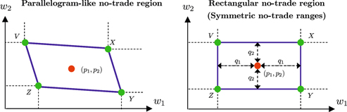
A parallelogram-like no-trade region is optimal for the asset allocation problem with transaction costs in general as in the left-hand side of Figure 15. On the other hand, we derive the optimal symmetric no-trade ranges (q1,q2) from a practical perspective, which is equivalent to rectangular regions where the policy asset mix (p1,p2) is the center of region as in the right-hand side of Figure 15.

Figure 15:

No-trade regions

In this section, we compare the constant and symmetric no-trade ranges in practical use with the general no-trade region for three-asset case (of two risky assets and a riskless asset). The baseline parameters in the analysis are shown in Table 4, used in Leland (1999) and Hibiki et al. (2014).

Table 4:

Baseline parameters

Expected rate of return	μ1=μ2=12.5%
Standard deviation	σ1=σ2=20%
Correlation	ρ12=0.2
Discount rate	r=7.5%
Proportional transaction costs	k1=k2=1%
Policy asset mix	p1∗=p2∗=0.4
Tracking error aversion	λ=1.3
Time interval and horizon	Δt=0.1, 10 years

We conduct the sensitivity analysis of the proportional transaction costs, the correlation coefficients, and the tracking error aversions. Ten kinds of values of each parameter in Table 5 are examined, and therefore 30 problems are solved in total.²²

Table 5:

Parameter values for the sensitivity analysis

	1	2	3	4	5	6	7	8	9	10
Transaction costs	0.1%	0.3%	0.5%	0.7%	1%	1.5%	2%	2.5%	3%	3.5%
Correlation	−0.3	–0.2	−0.1	0.0	0.1	0.2	0.3	0.4	0.5	0.6
TE aversion	0.5	1	1.3	2	3	4	5	10	20	30

^[1]

General case (Hibiki et al. 2014)

The results solved by the DFO method for the three-asset case of Leland model (1999) are obtained in Hibiki et al. (2014). Figure 16 shows the no-trade regions where the origin is the policy asset mix for the sensitivity analysis, and Figure 17 shows the mean no-trade ranges from the corner points to policy asset mix, which may be compared with the symmetric no-trade ranges in the section “Symmetric case”.

Figure 16:

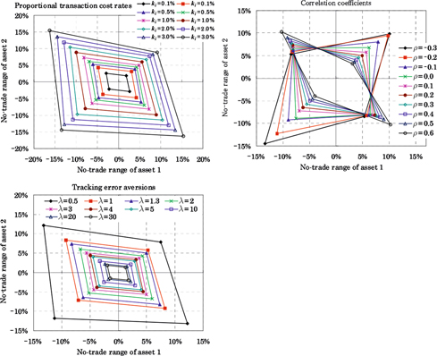
No-trade regions where the origin is the policy asset mix

Figure 17:

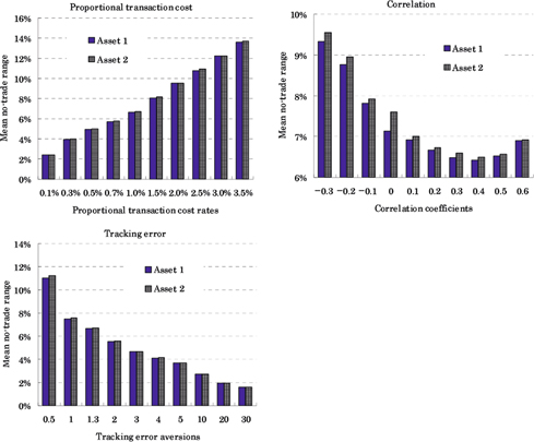
Mean no-trade ranges from the policy asset mix

As the proportional transaction cost rate becomes large, the no-trade region gets wider to avoid increasing the transaction cost. As the tracking error aversion becomes large, the no-trade region gets smaller to prevent losing touch with the policy asset mix. The shape of the no-trade region is a rectangle at zero correlation. The shape changes as the correlation deviates from zero. As the correlation becomes positively large, the shape of no-trade region is like a parallelogram which expands from top left to bottom right. As the correlation becomes negatively large, the shape of no-trade region expands from top right to bottom left.²³ When we change the parameters associated with the proportional transaction cost rates and the tracking error aversions, the mean no-trade ranges and the sizes of the no-trade regions vary in a similar way. However, the mean no-trade ranges are less sensitive to the correlation than other parameters while the shapes of the no-trade regions are more sensitive to the correlation.

Symmetric case

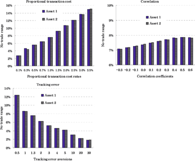
We calculate the optimal constant and symmetric no-trade ranges so that they can be obtained in the form of pi±qi%, where pi is the policy ratio of asset i and qi is the no-trade range of asset i. As in the section “General case (Hibiki et al. 2014)”, we show the results of the sensitivity analysis derived by the DFO method in Figure 18.

Figure 18:

No-trade ranges from the policy asset mix

As the proportional transaction cost rate becomes large, the no-trade region gets larger. As the tracking error aversion becomes large, the no-trade region gets smaller to avoid losing touch with the policy portfolio. These results are consistent with those of the average of the general no-trade ranges. However, in the case of sensitivity analysis for the correlation, the results of the symmetric no-trade ranges are different from the mean ranges in Figure 17 because the shapes of the general no-trade regions are sensitive to the correlations. In particular, the symmetric no-trade ranges are larger as the correlations are larger in the cases of less than the correlation of 0.5. The symmetric no-trade ranges are smaller after peaking at the correlation of 0.5. However, the symmetric no-trade ranges are not sensitive to the correlations. Therefore, we cannot reflect the influence of the different correlation to the no-trade ranges in the case that the no-trade ranges are symmetric.

The objective function values for the symmetric cases are larger than those for the general cases because the symmetric problems are solved under the constraints of the symmetric no-trade ranges. We show the increasing rates of the objective function values in Figure 19.

Figure 19:

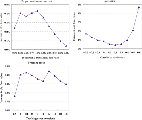
Increasing rates of the objective function values

The objective function values increase only about 0.5% in the case of the sensitivity analysis for the proportional transaction costs and the tracking error aversions. However, the objective function values increase between 0.5% and 5% in the case of the sensitivity analysis for the correlations. As the absolute values of correlations are large, the objective function values are larger because the no-trade regions change shape from the rectangle to the parallelogram. But the maximum increase in the objective function value is about 2% between –0.3 and 0.5 correlation coefficients.

Finally, we discuss the computation time. Average computation time is about 17 minutes for 30 general cases. Though it is acceptable computation time to solve the decision problem, we can solve the problem to decide the symmetric no-trade ranges only in about 90 seconds on average. Computation time decreases about 90%. The fact shows the use of the symmetric no-trade ranges is effective in the computational aspect.

Tracking error and mean-variance utility

We explain the rationale for modeling the trade-off between tracking error and transaction costs in our model by showing the relationship between tracking error and mean-variance utility in accordance with Leland (1999). At first, the mean-variance utility for N-asset case can be expressed as

[29]U(w)=μ⊤w−λw⊤Vw,

where μ∈ℝN is an expected return vector, V∈ℝN×N is a covariance matrix, w∈ℝN is a weight vector, and λ is a risk aversion.

The mean-variance utility maximization problem can be formulated as

[30]MaximizeU(w),

[31]subjecttoe⊤w=1,

where e=(1,1,…,1)T∈ℝN. The optimal solutions w∗ can be found using Lagrangian multiplier method as follow:

[32]w∗=12λV−1(μ−ηe),whereη=e⊤V−1μ−2λe⊤V−1e.

Suppose that the weight vector at time τ is w(τ)∈ℝN, and the trading weight vector is |Δw|.²⁴ The mean-variance utility can be expressed as

[33]U(w(τ))=μ⊤w(τ)−k⊤|Δw|−λw(τ)⊤Vw(τ),

for the problem with the proportional transaction cost because the transaction cost k⊤|Δw| is subtracted from the expected portfolio return μ⊤w(τ).

In this situation, investors will minimize the utility loss which is the difference between the mean-variance utility at w∗ and at w(τ), and it can be expressed in what follows.

[34]UL=U(w∗)−U(w(τ))=μ⊤w∗−λw∗⊤Vw∗−μ⊤w(τ)−k⊤|Δw|−λw(τ)⊤Vw(τ)=μ⊤(w∗−w(τ))−λw∗⊤Vw∗+λw(τ)⊤Vw(τ)+k⊤|Δw|

We substitute the optimal solutions [32] into eq. [34], and we obtain the following equation.

[35]UL=λ(w(τ)−w∗)⊤V(w(τ)−w∗)+k⊤|Δw|

The first term of eq. [35] shows tracking error, and the second term shows transaction cost. Though we need to pay attention to the fact that this can be applied to the simple mean-variance model, this is the rationale for modeling the trade-off between tracking error and transaction cost in our model as well as the Leland model (1999). Moreover, this would imply that we may choose the same “λ” as the risk aversion for the tracking error aversion.

References

Atkinson, C., and P.Ingpochai. 2010. “Optimization of N-Risky Asset Portfolios with Stochastic Variance and Transaction Costs.” Quantitative Finance10(5):503–14.10.1080/14697680903170791Search in Google Scholar

Boyle, P. P., and X.Lin. 1997. “Optimal Portfolio Selection with Transaction Costs.” North American Actuarial Journal1(2):27–39.10.1080/10920277.1997.10595602Search in Google Scholar

Conn, A. R., K.Scheinberg, and L. N.Vicente. 2009. “Introduction to Derivative-Free Optimization,” MPS-SIAM Series on Optimization.10.1137/1.9780898718768Search in Google Scholar

Chida, S. 2004. “Asset Management Strategy in Fujitsu Employees’ Pension Fund.” The Japan Pension Research Council, The 2004 General Assembly. (in Japanese) http://www.ier.hit-u.ac.jp/jprc/soukai2004/chida-paper.pdf.Search in Google Scholar

Donohue, C., and K.Yip. 2003. “Optimal Portfolio Rebalancing with Transaction Costs.” Journal of Portfolio Management29(4):49–63.10.3905/jpm.2003.319894Search in Google Scholar

Expert Committee on Economic Assumptions, Subcommittee for Pension Reform, the Social Security Council, Ministry of Health, Labour and Welfare. Subcommittee for Pension Reform, the Social Security Council, Ministry of Health, Labour and Welfare. 2008. “On the Subject of Range of Economic Assumptions on Financial Validation in 2009.” (in Japanese) http://www.mhlw.go.jp/shingi/2008/11/dl/s1111-5d.pdf.Search in Google Scholar

Gennotte, G., and A.Jung. 1994. “Investment Strategies under Transaction Costs: The Finite Horizon Case.” Management Science40(3):385–404.10.1287/mnsc.40.3.385Search in Google Scholar

Hibiki, N., R.Yamamoto, T.Tanabe, and Y.Imai. 2014. “Optimal Asset Allocation Strategy with Transaction Costs – Derivation of the Optimal No-Trade Region Using Derivative Free Optimization.” Transactions of the Operations Research Society of Japan57:1–26. (in Japanese)10.15807/torsj.1-26Search in Google Scholar

Leland, H. E. 1996. “Optimal Asset Rebalancing in the Presence of Transaction Costs,” Working Paper, U.C. Berkeley. http://www.haas.berkeley.edu/groups/finance/WP/9610004.pdf10.2139/ssrn.1060Search in Google Scholar

Leland, H. E. 1999. “Optimal Portfolio Management with Transactions Costs and Capital Gaines Taxes.” Working Paper, U.C. Berkeley. http://www.haas.berkeley.edu/groups/finance/WP/rpf290.pdf10.2139/ssrn.206871Search in Google Scholar

Liu, H. 2004. “Optimal Consumption and Investment with Transaction Costs and Multiple Risky Assets.” The Journal of Finance59(1):289–338.10.1111/j.1540-6261.2004.00634.xSearch in Google Scholar

Liu, H., and M.Loewenstein. 2002. “Optimal Portfolio Selection with Transaction Costs and Finite Horizons.” The Review of Financial Studies15(3):805–35.10.1093/rfs/15.3.805Search in Google Scholar

Lynch, A. W., and S.Tan. 2010. “Multiple Risky Assets, Transaction Costs, and Return Predictability: Allocation Rules and Implications for U.S. Investors.” Journal of Financial and Quantitative Analysis45(4):1015–53.10.1017/S0022109010000360Search in Google Scholar

Nocedal, J., and S. J.Wright. 2006. Numerical Optimization, 2nd ed.New York: Springer.Search in Google Scholar

NTT DATA Mathematical Systems Inc.2011. “NUOPT/DFO User Guide.” (in Japanese)Search in Google Scholar

Pliska, S. R., and K.Suzuki. 2004. “Optimal Tracking for Asset Allocation with Fixed and Proportional Transaction Costs.” Quantitative Finance4:223–43.10.1080/14697680400000027Search in Google Scholar

Sasaki, S. 2006. “Rebalancing for Policy Asset Mix.” Nissei Pension Strategy11:4–5. (in Japanese)Search in Google Scholar

1
The GPIF changed the midterm plan on June 7, 2013. The standard deviations and the correlation coefficients of the rates of returns of assets are recalculated and replaced while the expected rates of returns of assets are unchanged. As the results, the policy asset mix is modified as follows – 60% for domestic bond, 12% for domestic stock, 11% for international bond, 12% for international stock, and 5% for cash (unchanged). The permissible ranges are not changed. We use the values of Table 1 because our study is done before the change of the policy asset mix.
2
Many previous studies show that the optimal no-trade region is non-symmetric with respect to the policy asset mix or parallelogram-like policy (See Leland 1999; Liu 2004; Lynch and Tan 2010; Hibiki et al. 2014). We can compute the no-trade region and implement the rebalance strategy for two risky asset case. But four risky assets are usually invested for pension fund management, and therefore we use the symmetric no-trade ranges from a practical perspective. However, it is important to compare the results between the symmetric no-trade range (rectangular policy) and general no-trade region (parallelogram-like policy). We show the comparison for two risky asset case in the section “Comparison of the symmetric case with the general case”.
3
We show the rationale for using the trade-off between tracking error and transaction cost in the no-trade range problem in accordance with Leland (1999) in the section “Tracking error and mean-variance utility”.
4
The no-trade boundary is the optimal rebalance target in the infinite and continuous-time model with proportional transaction costs as in Leland (1999), but we cannot guarantee it in the finite and discrete-time model. However, Hibiki et al. (2014) showed that the boundary value of the no-trade range is still appropriate as the rebalance target for two-asset case with a risky asset and a riskless asset, and therefore we define the problem based on the rebalance strategy from a practical perspective.
5
The readers can refer Conn, Scheinberg, and Vicente (2009) and the chapter nine of Nocedal and Wright (2006) in detail. In this paper, we use NUOPT/DFO (2011) added on the mathematical programming software package called NUOPT developed by NTT DATA Mathematical Systems, Inc. NUOPT/DFO implements the trust-region methods based on derivative-free models, which maintain quadratic models based only on the objective function values computed at sample points.
6
In the case of the GPIF as in Table 1, the asset N is short-term asset or cash. We need to have cash in a degree in order to pay for pension money, while we need to invest in risky assets without having much cash because of the efficient investment. When we do not impose the boundary constraints, we have LN=0 and UN=1.
7
We do not need to adjust the risky assets within the no-trade ranges in the continuous-time model because even the asset out of the no-trade range is rebalanced on the boundary immediately. However, we need to adjust the risky assets within the no-trade ranges even in the continuous-time model if the lower bound of asset N is greater than zero, that is LN>0.
8
If the no-trade ranges are small, we do not need to adjust the amounts of assets; however, we need to pay much transaction costs. Therefore, the optimal no-trade ranges are derived in consideration of the trade-off.
9
Our procedure may be complicated. The reason is we impose the constraints (or upper and lower limits) for cash. However, according to the numerical analysis (the left graph of Figure 6) in Section 3.1, the probabilities of which cash is adjusted due to the constraints are at most about 6% for Δt=0.1 year and about 14% for Δt=1.
10
The investment value is not dependent on path m at time 0, but we describe the notation for convenience.
11
As in eq. [11], the decreases in the asset weights except the assets in the set It+(m) and asset N are equal to zero.
12
The weight of asset N is wNta(m)={LN for EWt(m)>0UN for DWt(m)>01−∑i∈IN−1wita(m) otherwise.
13
They calculate three kinds of estimates for the appreciation rates for total factor productivity; 1.3%, 1.0%, and 0.7%. They estimate the different expected rates of returns, respectively.
14
The transaction costs used by the GPIF are not published, and there are a few previous studies which describe the transaction costs. Sasaki (2006) sets 0.5% for stocks and 0.2% for bonds. Chida (2004) sets 1.2% for stocks and 0.2% for bonds as the transaction cost rates including market impact costs. In this paper, we use the rates in Chida (2004). We set the tracking error aversion to three (λ=3) from the following reason. As shown in the section “Tracking error and mean-variance utility”, we may choose the same value as the risk aversion for the tracking error aversion in the case of the simple mean-variance problem. It is published that the policy asset mix is derived by solving the mean-variance optimization problem with the parameters in Table 3 under the constraints that the expected rate of return is equal to 4.1%. The reciprocal of the dual value for the constraint corresponds to the risk aversion of the objective function which consists of the expected value and the variance of the rate of return, and the risk aversion is 2.99. The mean-variance optimization problem for the GPIF is different from the problem shown in the section “Tracking error and mean-variance utility” because of adding some constraints. Unfortunately, we have no idea to determine the appropriate value of λ except the simple mean-variance problem. Therefore, we approximately assigned three (λ=3) to the tracking error aversion.
15
The number of periods is calculated by years divided by the time intervals. For example, the number of periods is 100 when Δt=0.1 and 10 year horizon.
16
Figure 7 shows that the no-trade ranges become wide as the proportional transaction cost rates increase. The no-trade ranges of the stocks become wide relatively to the bonds because the proportional transaction cost rates of the stocks are 1.2%, and those of the bonds are 0.2%. The no-trade range is more affected by the target ratio than the proportional transaction cost for the domestic bond. We conduct the sensitivity analysis for the proportional transaction cost in detail in Section 3.2.
17
The GPIF uses the following constraints to derive the target portfolio; the target ratio of short-term asset (cash) = 5%, the expected rate of return of the target portfolio = 4.1%, and the relationship among the target weights of the assets is DS>IS>IB. In particular, we impose constraints on the above-mentioned relationship among asset weights as follows: DSweight≥ISweight+1% and ISweight≥IBweight+1%. We solve the problem by the mean-variance model and obtain the optimal weights of 66.7% for DB, 10.4% for DS, 8.4% for IB and 9.4% for IS. When we round the weights to 1% unit, the weights of the target portfolio in Table 1 are obtained. The policy portfolio is the P3 portfolio. The other portfolios (P1 to P10 except P3) can be also derived by solving the mean-variance problems with the expected rates of returns of 3.9%, 4.0%, 4.3%, 4.5%, 4.7%, 4.9%, 5.1%, 5.3% and 5.5%, respectively.
18
The GPIF has managed their investment assets using the no-trade ranges in Table 1 since March 2008.
19
Four cases are IS in December 2012 for 5 year problem, IS in September and December 2012 for 50 year problem, and DB and IB in December 2012 for 50 year problem. The probability of the violation is 1.25% (=1/80) for 5 year problem, and 3.75% (=3/80) for 50 year problem.
20
It is difficult to evaluate the validity of the optimal ranges because the optimal values depend on the parameters such as the proportional transaction costs and the tracking error aversions. This is one of the ways to evaluate the validity.
21
Technically, it depends on the values of β and γ.
22
When we examine the sensitivity of the proportional transaction costs, ten cases are solved under correlation of 0.2 and tracking error aversion of 1.3 as in Table 4.
23
The shape of the no-trade region is square in the zero correlation case because the parameters of both assets are same. The shapes are like rhombus in the non-zero correlation cases.
24
The weight vector before trading assets is either w(τ)+Δw or w(τ)−Δw at time τ.

Published Online: 2014-6-24

Published in Print: 2014-7-1

You are currently not able to access this content.

Articles in the same Issue

https://doi.org/10.1515/apjri-2013-0024

Keywords for this article

asset allocation; transaction cost; no-trade range; derivative-free optimization