The Optimal Strategy of Reinsurance-Investment Problem for an Insurer with Dynamic Income Under Stochastic Interest Rate
-
Delei Sheng


Abstract
This paper considers the reinsurance-investment problem for an insurer with dynamic income to balance the profit of insurance company and policy-holders. The insurer’s dynamic income is given by a net premium minus a dynamic reward budget item and the net premium is obtained according to the expected premium principle. Applying the stochastic control technique, a Hamilton-Jacobi-Bellman equation is established under stochastic interest rate model and the explicit solution is obtained by maximizing the insurer’s power utility of terminal wealth. In addition, the comparison with corresponding results under constant interest rate helps us to understand the role and influence of stochastic interest rates more in-depth.
1 Introduction
Existing literatures investigate the optimal reinsurance-investment problem only from the view of insurer, but lack of meticulous care to balance the profit of both insurance company and policy-holders. An effective way to balance both profits of insurer and policy-holders is reward budget. The reward budget is a dynamic item which can be subtracted from the actuarial premium income. As a consequence, insurer’s income is dynamic, which given by an actuarial income under classic premium principle minus a dynamic reward budget item.
Portfolio has been a popular research field for more than sixty years after Markowitz’s pioneering work. It is still a very interesting problem which attracts a lot of research work in recent years. For example, Bjork, Murgoci, Zhou[1] gave a more realistic model for the case when the risk aversion depends dynamically on current wealth and studied the mean–variance portfolio optimization to find the optimal time consistent strategy. Zhu[2] studied the uncertain optimal control problem by applying Bellman’s principle of optimality and used the equation of optimality to solve a portfolio selection model. Hu, Øksendal, and Sulem[3] presented a mathematical model for a Black–Scholes market driven by fractional Brownian motion and found explicitly the optimal consumption rate and the optimal portfolio in such a market for an agent with utility of power functions. Cao and Xu[4] derived the forms of proportional and excess-of-loss reinsurance contracts under the assumption that investment fund follows the logarithm-normal distribution. Countless earlier literature need not too much listed here.
However, very few studies on the portfolio optimization under the stochastic interest rates before and small amount of literature emerges in nearly more than a decade. Korn and Kraft[5] considered investment problems under a stochastic interest rate to maximize her utility from terminal wealth without the usual Lipschitz assumptions. Grasselli[6] studied an investment problem for the HARA utility functions assuming the interest rates following the Cox-Ingersoll-Ross dynamics. Pang[7] considered a portfolio optimization problem on an infinite time horizon by maximizing the infinite horizon expected discounted log utility of consumption when the interest rate described by an ergodic Markov diffusion process. Li and Wu[8] obtained a closed-form expression of the optimal policy that maximizes a power utility for the optimal investment problem under the stochastic interest rate formulated as CIR model. Guan and Liang[9] investigated an optimal investment strategy of DC pension plan in the stochastic interest rate and stochastic volatility framework. They also investigated the optimal reinsurance and investment problem[10] when interest rate risk and inflation risk are considered in the same year.
In this paper, we study the optimal reinsurance strategy and investment strategy for an insurer with dynamic income under Ho-Lee stochastic interest rate model. A Hamilton-Jacobi-Bellman equation is established and the explicit solution for the HJB equation is obtained by maximizing the insurer’s power utility of terminal wealth. At last, some numerical simulations and graphics are given to show the impacts of different parameters. By contrast, the results under Ho-Lee model are always higher than results under constant interest rate.
The remainder of this paper is organized as follows. In Section 2, we formulate a general framework and give some models will be used hereinafter. In Section 3, a Hamilton-Jacobi-Bellman equation is established and the explicit solution has been obtained. At last, numerical simulations and graphics are provided in Section 4.
2 Formulation of the Model
Throughout this paper, (Ω, ℱ, P, {ℱt}0 ≤ t ≤ T) denotes a complete probability space satisfying the usual condition, where T > 0 is a finite constant representing the investment time horizon; ℱt stands for the information available until time t.
2.1 The Financial Market
We consider a financial market in which transaction amounts are so small that we can consider they have no influence on the prices, and the market with no arbitrage, frictionless, and continuously open as well.
Without loss of generality, we assume that the financial market is composed of two kinds of assets: Cash and equities. For the sake of simplicity, we will only consider one equity asset which can indeed represent the index of a stock market.
The instantaneous risk-free rate r(t) followed by the stochastic interest rate models of constant volatility, which described by the Ho and Lee[11] model
where
The price S0(t) of the cash asset is given by
Here r(t) is the stochastic interest rate.
The stock market index price S(t) at time t ≥ 0 can be described by the model
where u(t) is another positive real-valued function, and the constant v > 0 denotes the volatility rate of risk asset. Two Brownian motions satisfying E[
In the financial model (2), u(t) > 0 is a natural hypothesis, which means that the investment on stock can make more money than investing on cash asset, which is consistent with the economic principle of high-risk high-yield. In fact, only when u(t) > 0, more people are willing to invest on equities.
2.2 The Surplus Process of Insurer
We use the classical Cramer–Lunderburg model to describe the surplus process of insurer.
where N(t) is a homogeneous Poisson process with intensity λ, the claim sizes {Yi,i ≥ 1} are independent and identically distributed positive random variables with E[Yi] = μ and
The diffusion approximation of the compound poisson process
where W(t) is a standard Brownian motion and independent with
In order to avoid unbearable risk, the insurance company can buy proportional reinsurance to transfer part of the potential risk to reinsurance company. The insurer’s retention proportion is p ∈ [0, 1], the remaining 1 − p shall be borne by the reinsurer. 0 ≤ θ ≤ η ≤ 1 is the safety loading of reinsurer.
In the above equation, ηpλμ − (η − θ)λμ = c − (1 + η)(1 − p)λ μ − pλμ is a difference after reinsurance premium and average claim size being subtracted from the net premium.
A new notation
2.3 The Insurer’s Wealth Process with Dynamic Income
The proportion of wealth invested on stock asset denoted by π(t) which is a progressively measurable real function, X(t) with X(0) = x0 represents the wealth of the insurer, then we have
The dynamic income of an insurer is equal to the net premium according to premium principle minus reward budget. Here, the dynamic income of insurer is (1 + θ)λ μ − kX(t), where k is the reward budget coefficient and (1 + θ)λμ is the insurer’s net premium according to expected premium principle. The central element which makes the insurer’s income be dynamic is the reward budget which change with the dynamic process of insurer’s wealth. To determine the reward budget coefficient is a prudent event for any insurer, the reward budget deducted from premium income at a fixed share depend on both bygone experience and prospective prognosis.
A strategy α = (p(t), π (t)) is said to be admissible, if ∀ t∈ [0, T], α is ℱ(t) progressively measurable and
3 Main Results
In this subsection, we consider the reinsurance-investment problem with stochastic interest rate. Assuming the insurer’s objective is to maximize the expected utility from terminal wealth, where the utility U(x) is a power utility (constant relative risk aversion) function U(x) = xδ, the constant δ ∈ (0, 1) is the relative risk aversion coefficient of a risk averse insurer. This utility function plays a vital role in actuarial mathematics and insurance practice. For an admissible strategy α = (p(t), π (t)), the value function Jα(t,x,r) from state (x, r) at time t is defined as
and the optimal value function is given by
with the boundary condition
The goal of the insurer is to find an optimal strategy α* = (p*(t), π*(t)) such that Jα*(t, x, r) = H(t, x, r), where p*(t) is called the optimal reinsurance strategy and π*(t) is called the optimal investment strategy.
3.1 An Insurer with Reward Budget Under the Ho-Lee Model
If the stochastic interest rate followed by the Ho-Lee model
For any H(t, x, r) ∈ C1,2,2([0, T] × R+ × R+), according to the classical results of Fleming and Soner[12], the generator can be defined as a variational operator
where Ht, Hx, Hr, Hxx, Hrr and Hxr denote the corresponding first and second-order partial derivatives with respect to (w.r.t.) the corresponding variables t, x, r, respectively. The Hamilton-Jacobi-Bellman (HJB) equation for problem (6) is given by
with the boundary condition (7).
In the remainder of this section, we try to find the explicit solutions to problem (6) with stochastic interest by stochastic control technique.
Theorem 1
For the optimal control problem(6), assume that the objective is to maximize utility of terminal wealth, at the fixed terminal time T, and the power utility function is given by
The optimal investment strategy is
Proof
The HJB equation (8) rewritten by
According to the first-order necessary conditions of the extremum, the optimal strategies
Inserting (12) and (13) into (11), the HJB equation becomes
Conjecture of the solution has the following form
The derivatives of the conjecture with respect to t, x, r, respectively.
Plugging these derivatives into (14)
Splitting (16) into two equations
i.e.,
The solution of (17) is
The solution of (20)
Plugging (21) and (19) into (15), the optimal value function is obtained.
Plugging (19) into (12) and (13), respectively. The optimal strategy (p*, π*)
The proof is finished.
Remark 1
For the optimal investment strategy (9)
where u(t) > 0 is a positive real-valued function and the constant b > 0 is the volatility of interest rate. The proportion
Observed carefully from the model (2) and (1), we conclude that u(t) is the excess-appreciate-rate of stock relative to cash. The principal parts of the optimal investment strategy π* are two components: one is the relative proportion
In other words, the optimal investment strategy π* is mainly determined by two components: the relative ratio of stock’s excess-appreciate-rate divided by the stock’s volatility rate and the volatility rate of stochastic interest.
Remark 2
For the optimal reinsurance strategy (10), if we let m = λμ which represents mean-value of insurer’s claim size and
It’s nature that the optimal reinsurance strategy p* increases with respect to the wealth level at time t. The most interesting discovery is that we find the optimal reinsurance strategy mainly determined by
Corollary 1
Assuming that the objective is to maximize utility of terminal wealth, at the fixed terminal time T, and the power utility function is given by
If a(t) = a > 0 andu(t) = u > 0, where a and u are constants, the control problem(6)has a simple version, then the optimal value function is given by in simple form
Proof
In fact, if the deterministic function a(t) = a > 0 and u(t) = u > 0, where a and u are constants, similar to the above proof completely, we obtain that f(t) can be given in more simple form.
and h(t) = (1 − k) δ (T − t). So the desired value function and optimal strategy are obtained.
Theorem 2
(verification theorem) Let H(t,x,r) be a convex, twice differential solution to(8)with the boundary condition(7)such that |H(0, x0, r0)| < ∞. Then, for all t ∈ [0, T], x ∈ (0, ∞),
H(t, x, r) ≤ Jα(t, x, r) for every admissible strategy α.
If there exists an admissible control α* = (p*, π*) such that
then the value function H(t,x,r) = Jα*(t, x, r) and the policy α* = (p*, π*) is the optimal strategy corresponding to Xα*(t) which is the solution of(5).
3.3 A Special Case of an Insurer with Reward Budget Under a Constant Interest Rate
In this subsection, we investigate a special case that the interest rate r(t) is a constant r. All assumptions are the same as above except that r(t) ≡ r throughout this part, thus we have
and
where r, v are positive constants, u(t) is a positive real-valued function. The surplus processes with claim and reinsurance are the same as (3) and (4), W(t) and
The utility U(x) is also a power utility (constant relative risk aversion) function U(x) = xδ to maximize the expected utility of terminal wealth, where the constant δ ∈ (0, 1) is the relative risk aversion coefficient of a risk averse insurer. For the optimal control problem
with the boundary condition H(T,x,r) = xδ.
Applying the classical tools of stochastic optimal control, if the optimal value function H(t,x) ∈ C1,2([0, T]× R), then H satisfies the following Hamilton-Jacobi-Bellman (HJB) equation:
According to the first order necessary condition of extreme, we obtain that
Conjecture of the solution has the following form
Through the similar calculation as before, we obtain the value function
and the optimal strategy α* = (p*, π*) as follows:
Remark 3
Comparing the results of constant interest rate with the results of stochastic interest rate, it is easy to find that the optimal strategy under the stochastic interest rate exists one term more than the optimal strategy under a constant interest rate.
If ρ1 > 0, then p* stochastic > p* constant, else if ρ1 < 0, then p* stochastic < p* constant.
Let’s pay attention to
Similarly,
If ρ2 > 0, then π* stochastic > π* constant, else if ρ2 < 0, then π* stochastic < π* constant.
It is noteworthy that
In one word, whether the expression
4 Numerical Simulations
In this section we illustrate some experiments on simulated data for the case of u(t) = u and a(t) = a where u and a are positive constants. Unless otherwise stated, the related model parameters are as follows:
Numerical values of parameters
| x | η | λ | μ | b | v | u | k | T | δ | σ | ρ1 | ρ2 | a |
|---|---|---|---|---|---|---|---|---|---|---|---|---|---|
| 3 | 0.1 | 2 | 0.2 | 0.1 | 0.1 | 0.15 | 0.05 | 10 | 0.5 | 2 | 0.3 | 0.1 | 0.06 |
First, we propose two experiments to study the optimal value function, the one to analyze the formula (22) under the stochastic interest rate and the other to analyze the formulas of (23) under a constant interest rate. The simulations mainly focus on the changes of the value function with respect to x, t, r, u, respectively. See Figure 1, Figure 2, Figure 3 and Figure 4.


The analysis below will always be a comparison of the results under the stochastic interest rate and the corresponding results under a constant interest rate. Each numerical graphic consists of two curves, dashed line representing the result under the stochastic interest rates and solid line representing the result under the constant interest rate. With the curve under constant interest rate as reference, it can help us to understand the role and influence of stochastic interest rates more clearly and more in-depth.
Figure 1 shows that the value function increases as the wealth level increasing, but the speed becoming slower and slower. This is the basic characteristics of utility function. The results obtained in line with the features of utility function, which confirms the correctness of our result.
Figure 2 shows the trend that the value function changes with time. When other parameters determined, you can see that the utility under the stochastic interest rate decreases with time but there is little change of the utility under a constant interest rate.
Figure 3 and Figure 4 shows the utility increases with the return level. Both the increase of interest rate r and the increase in risk premium u will lead to a significant increase in utility.
But the utility increasing with risk premia is more significant.
In the following, let’s review the optimal strategy α* = (p*, π*) with a constant interest rate
and the optimal strategy α* = (p*, π*) with stochastic interest rate
The rest of this part mainly focus on the analysis and comparisons of the optimal strategies, which will be illustrated through several graphics.
For the optimal reinsurance proportion p*, the simulations mainly focus on the changes with respect to x, δ, μ, σ, respectively. See Figure 5, Figure 6, Figure 7 and Figure 8.

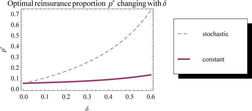


Figure 5 shows that whether a constant interest rate or a stochastic interest rate, the optimal reinsurance proportion always increases with the wealth level x. But the trend under the stochastic interest rate is more significant, which in turn suggests that the growth of insurer’s wealth under stochastic interest rates need to bear even greater risk.
Figure 6 reflects the sensitivity of the reinsurance proportion on the degree of risk aversion. Figure 7 and Figure 8 show the trend of reinsurance proportion changing with the claim size and the claim volatility, respectively.
For the optimal investment strategy π*, the simulations mainly focus on the changes with respect to u, v, k, δ, respectively. See Figure 9, Figure 10, Figure 11 and Figure 12.


Figure 9 and Figure 10 show the trend of investment strategy changing with the risk premium u and the risk volatility v, respectively. Figure 11 shows that the reward budget increasing inevitably leads to the increase of the risk investment share. The increase of investment income can make up for the increase of budget share. Figure 12 shows the impacts of risk preference on the investment share.
Remark 4
Overall, the curve under the stochastic interest rate is always above the corresponding curve under a constant interest rate. Comparing with constant interest rate, the stochastic interest rate brings more risk into the wealth process, so that the insurer has to transfer more of the risk to the reinsurer and the reinsurance proportion p will be higher. However, transferring more risks to reinsurer must increase the insurance company’s spending, which requires insurer to seek much greater investment return. This eventually leads to a further increase of the investment share π on risk asset.
5 Conclusion
Based on the viewpoint of interaction between insurance company and policy-holder, we introduce reward budget into the insurance risk management process in this paper, which makes the insurer’s income to be dynamic. Some results are obtained under the stochastic interest rate model, but the follow-up work remains to be further perfect.
Supported by the National Natural Science Foundation of China (11301376)
Acknowledgements
We thank the referees for their time and comments.
References
[1] Bjork T, Murgoci A, Zhou X Y. mean-varicance portfolio optimization with state-dependent risk aversion. Mathematical Finance, 2014, 24(1): 1–24.10.1111/j.1467-9965.2011.00515.xSearch in Google Scholar
[2] Zhu Y. Uncertain optimal control with application to a portfolio selection model. Cybernetics and Systems, 2010, 41(7): 535–547.10.1080/01969722.2010.511552Search in Google Scholar
[3] Hu Y, Øksendal B, Sulem A. Optimal consumption and portfolio in a Black-Scholes market driven by fractional Brownian motion. Infinite Dimensional Analysis Quantum Probability and Related Topics, 2011, 6(4): 519–536.10.1142/S0219025703001432Search in Google Scholar
[4] Cao Y, Xu J. Proportional and excess-of-loss reinsurance under investment gains. Applied Mathematics and Computation, 2010, 217(6): 2546–2550.10.1016/j.amc.2010.07.067Search in Google Scholar
[5] Korn R, Kraft H. A stochastic control approach to portfolio problems with stochastic interest rates. SIAM Journal on Control and Optimization, 2002, 40(4): 1250–1269.10.1137/S0363012900377791Search in Google Scholar
[6] Grasselli M. A stability result for the HARA class with stochastic interest rates. Insurance: Mathematics and Economics, 2003, 33(3): 611–627.10.1016/j.insmatheco.2003.09.003Search in Google Scholar
[7] Pang T. Stochastic Portfolio Optimization with Log Utility. International Journal of Theoretical and Applied Finance, 2006, 9(6): 869–887.10.1142/S0219024906003858Search in Google Scholar
[8] Li J, Wu R. Optimal investment problem with stochastic interest rate and stochastic volatility: Maximizing a power utility. Applied Stochastic Models in Business and Industry, 2009, 25(3): 407–420.10.1002/asmb.759Search in Google Scholar
[9] Guan G, Liang Z. Optimal management of DC pension plan in a stochastic interest rate and stochastic volatility framework. Insurance: Mathematics and Economics, 2014, 57(6): 58–66.10.1016/j.insmatheco.2014.05.004Search in Google Scholar
[10] Guan G, Liang Z. Optimal reinsurance and investment strategies for insurer under interest rate and inflation risks. Insurance Math. Econom., 2014, 55(1): 105–115.10.1016/j.insmatheco.2014.01.007Search in Google Scholar
[11] Ho T S Y, Lee S B. Term structure movements and pricing interest rate contingent claims. Journal of Finance, 1986, 41(5): 1011–1029.10.1111/j.1540-6261.1986.tb02528.xSearch in Google Scholar
[12] Fleming W H, Soner H M. Controlled Markov Processes and Viscosity Solutions. Springer, Berlin, 1993.Search in Google Scholar
[13] Gu A, Guo X, Li Z, et al. Optimal control of excess-of-loss reinsurance and investment for insurers under a CEV model. Insurance: Mathematics and Economics, 2012, 51(3): 674–684.10.1016/j.insmatheco.2012.09.003Search in Google Scholar
© 2016 Walter de Gruyter GmbH, Berlin/Boston
Articles in the same Issue
- Capability Oriented Combat System of Systems Networked Modeling and Analyzing
- Development and Evolution of Aluminum Industry in China Based on Aluminum Flow Analysis
- A Study on the Rapid Parameter Estimation and the Grey Prediction in Richards Model
- Does Medical Insurance Improve Household Consumption in China? — A Re-analysis Based on Meta Regression Analysis
- The Optimal Strategy of Reinsurance-Investment Problem for an Insurer with Dynamic Income Under Stochastic Interest Rate
- Group Consensus of Second-Order Dynamic Multi-Agent Systems with Time-Varying Communication Delays and Directed Networks
- A Generalized Constant Elasticity of Substitution Production Function Model and Its Application
- Fuzzy Integral Multiple Criteria Decision Making Method Based on Fuzzy Preference Relation on Alternatives