
Effect of concentration dependence of viscosity on squeeze film lubrication
-
Poosan Muthu
 and
Vanacharla Pujitha
and
Vanacharla Pujitha

Abstract
The influence of concentration of solute particles on squeeze film lubrication between two poroelastic surfaces has been analyzed using a mathematical model. Newtonian viscous fluid is considered as a lubricant whose viscosity varies linearly with concentration of suspended solute particles. Convection-diffusion model is proposed to study the concentration of solute particles and is solved using finite difference method of Crank–Nicolson scheme. An iterative procedure is used to get the solution for concentration, pressure and velocity components in film region. It has been observed that load carrying capacity decreases as the concentration of solute particles in the fluid film decreases. Further, the concentration of suspended solute particles decreases as the permeability of the poroelastic plate increases and these results may be useful in understanding the mechanism of human joint.
1 Introduction
Lubrication is a process by which friction and wear between two moving surfaces are reduced by a suitable substance called as lubricant. We can observe the lubrication process in machines, human body and other systems. Synovial joints are weight bearing systems in the human body with low frictional coefficient and wear in comparison with mechanical bearings [1].
Synovial joint is a connection between two moving bones consisting of a cartilage lined cavity filled with a lubricant called as synovial fluid. The behavior of synovial joint is mainly governed by the properties of synovial fluid and articular cartilage. The articular cartilage exhibits elastic behavior and is slightly permeable. The principal role of synovial fluid is to reduce friction between two moving articular cartilage surfaces. Its viscosity is due to the presence of hyaluronic acid (HA) molecules in it. In normal joints, these acid molecules cannot pass through the articular cartilage [2].
Torzilli and Mow [3] studied theoretically the characteristics of articular cartilage and synovial fluid. Bujurke et al. [4] have analyzed the squeeze film lubrication of synovial joint using a mathematical model by considering the lubricant as second-order fluid and cartilage as a porous surface. Hou et al. [5] have studied the lubrication mechanism of articular cartilage. Squeeze film lubrication of synovial joint with Bingham fluid as a lubricant and cartilage as a two layered porous region is mathematically modeled by Tandon et al. [6]. Bujurke and Kudenatti [7] have studied the effect of surface roughness and poroelastic behavior of cartilage on lubrication mechanism of joint. From all these research articles one can observe that load carrying capacity and pressure are important physical quantities in the study of lubrication mechanism. These quantities decrease with increasing values of permeability of the porous surface and increase with increasing values of elastic parameter.
Walker et al. [8] proposed the concept of boosted lubrication in load bearing phase of synovial joint. It is mentioned that when two bones approach each other, water and low molecular weight molecules pass through the cartilage surface and the HA molecules remain in the joint cavity. Due to the presence and increase in the concentration of acid molecules, the joint supports more load. Tannin et al. [9] experimentally investigated that presence of HA in synovial fluid reduces coefficient of friction in joint. Collins [10] analyzed the gel formation of HA molecules in joint. Tandon et al. [11] studied the lubricant gelling in synovial joint during articulation with viscoelastic fluid as lubricant. Mathematical model on dispersion of acid molecules and nutrients transport in the articular cartilage is useful in understanding the mechanism of synovial joint [12]. These studies modeled the effect of HA molecules on joint mechanism, assuming constant viscosity coefficient. But, the coefficient of viscosity of the synovial fluid changes with concentration of acid molecules present in it.
Recently, studies have been carried out to model the synovial fluid flow in rectangular cavity [13], [14]. In these investigations, the following assumptions are made: (i) viscosity depends on concentration and shear rate and (ii) shear-thinning index depends on concentration. But, geometry considered in the study is not relevant to biological synovial joint. That is, surfaces are rigid and flat. In nature, the joint surfaces are poroelastic. Further, the effect of concentration of HA molecules on pressure and load carrying capacity is not investigated in these articles.
Morris et al. [15] reported that the viscosity of synovial fluid increases rapidly and exponentially with concentration of HA molecules. Mathematical model describing the combined effect of variation of viscosity with concentration of HA and poroelastic nature of cartilage surface on lubrication of joint is not available in the literature. Hence, the main purpose of the present paper is to study the effect of concentration of solute particles on squeeze film lubrication between two poroelastic surfaces, assuming variable viscosity coefficient with respect to concentration.
2 Mathematical formulation
Figure 1 is the geometrical representation of model of synovial joint under consideration along with cartesian coordinate system
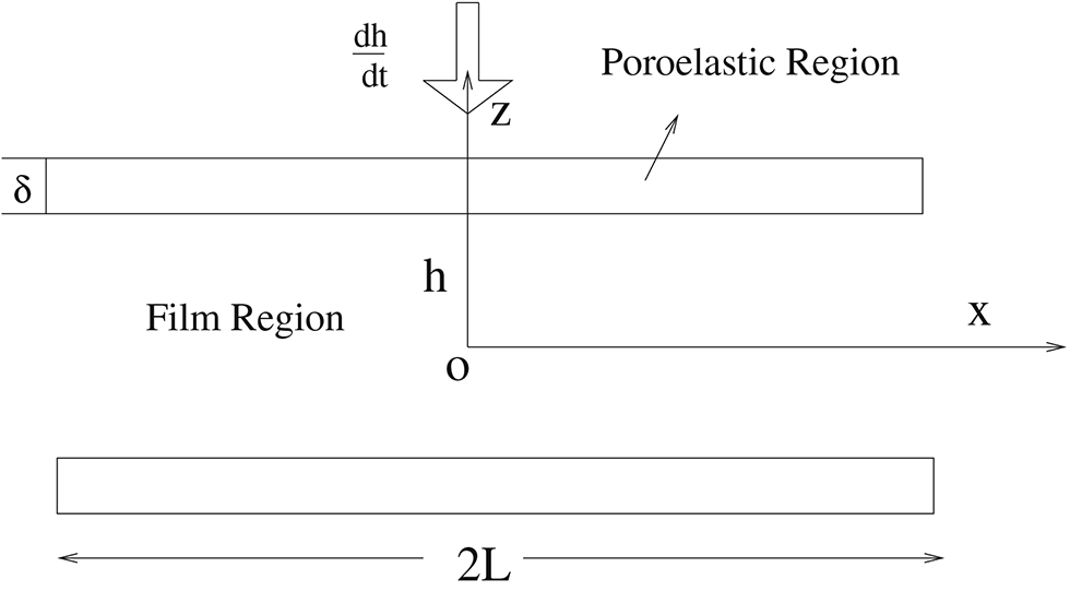
Geometry of the present problem.
The assumptions involved in mathematical formulation of the problem are listed below: In the film region, Newtonian viscous fluid is taken as lubricant, whose viscosity varies with concentration of HA. Fluid flow is laminar. Body forces are neglected. Fluid inertia is small compared to viscous shear. The height of the fluid film h is very small compared to the length L. Since squeeze film thickness is smaller than the length of the plates, variation of pressure across the fluid film is insignificant. Compared with the velocity gradient
Film region:
where
Ferguson et al. [19] experimentally proved that the viscosity of the synovial fluid linearly depends on concentration of HA. Accordingly, we assume that the coefficient of viscosity (μ) depends upon the concentration, as given in the following expression [2], [19],
where λ is constant and
In poroelastic region, the fluid is assumed to be Newtonian fluid with constant viscosity
Poroelastic region:
where
where
Adding Eqs (10) and (11) and using Eqs (8) and (9), we get
The divergence of Eq. (12) gives
We define cartilage dilatation in terms of average bulk modulus K as given in [20],
We get equation of pressure in poroelastic region by substituting Eq. (14) in (13) as,
Next, we will derive the equation corresponding to the pressure in film region, using velocity components u and w. For which, the governing Eqs (1) and (2) are solved to get solution for u and w, using suitable boundary conditions as given below.
Boundary conditions:
The boundary conditions for velocity field are:
At the axis of symmetry:
(16)At the permeable wall, the tangential velocity
The boundary conditions for concentration of solute particles in fluid film region are:
At middle of the channel
(18)where
At the symmetry plane :
(19)Solute mass flux at the permeable wall is given by [21] :
(20)
The solute flux through the interface is given by the boundary condition (20). The solute flux by diffusion process is given by product of permeability of solute at the wall
3 Solution
Solution of velocity component (u) is obtained by integrating the
Solution of normal velocity component (w) is obtained by substituting the velocity u in the continuity Eq. (1) and integrating it with respect to z. Further, applying boundary condition (16) on w and following Leibnitz rule, we get,
Substituting the velocity component u in the continuity Eq. (1) and integrating it over the film thickness from
After neglecting the inertia term in Eq. (7), we have
Substitution of Eq. (14) in Eq. (24), gives
Now
Integrating the Laplace Eq. (15) with respect to z over porous matrix thickness from
If the thickness of porous layer (δ) is assumed to be of very small then Eq. (27) reduces to
Eq. (28) is valid in the limiting case when
Therefore,
Substituting Eq. (29) in Reynolds Eq. (23), we get equation for pressure in film region as,
Solution for pressure in the film region can be obtained by solving Eq. (30) along with boundary conditions given below.
Boundary conditions for Pressure:
At middle of the channel :
(31)At end of the channel :
Integrating Eq. (30) with respect to x twice and using boundary conditions (31) and (32) we get pressure in the dimensional form as,
We define the following non-dimensional quantities
to get the dimensionless form of the Eqs (4), (5), (21), (22) and (33).
We get the non-dimensional pressure in the film region as, after dropping bar,
The convection diffusion Eq. (4) and corresponding initial and boundary conditions (18), (19) and (20) are written in non-dimensional form (after removing bar) as :
where
Non-dimensional form of velocity components and viscosity (after removing bar) are
Now, we solve Eq. (35), which is coupled with Eqs (34), (39), (40) and (41). It is not possible to solve the Eq. (35) analytically, along with u, v and p quantities. Hence, Eq. (35) is solved numerically along with initial and boundary conditions (36), (37) and (38), in an iterative manner.
3.1 Numerical procedure
Finite difference method of Crank–Nicolson scheme is used to solve the convection-diffusion Eq. (35) along with the initial and boundary conditions (36)–(38), to get concentration value
where coefficients
To obtain the solute concentration value at the symmetric plane
To calculate solute concentration values at top boundary, we discretize the boundary condition (38) by using three point backward difference formula [23]. Hence, at
Thomas algorithm is used to solve the system of linear Eqs (42)–(44). The solutions for concentration (c), velocity components (u, w) and pressure (p) are obtained using an iterative procedure.
Solution procedure is started by assuming an approximate value for
Once the correct c value for all grid points is obtained, then the fluid viscosity and the squeeze film pressure are calculated numerically using Eqs. (41) and (34), respectively. Further, the non-dimensional form of load carrying capacity can be obtained by integrating this pressure p over the film region. It is expressed as:
4 Results and discussion
The objective of this analysis is to study the effect of solute concentration on squeeze film lubrication between two poroelastic surfaces. This study may be useful in understanding the lubrication mechanism of joint due to the following reason When the articular cartilages move closer to each other, water and low molecular solutes may press out from joint cavity into cartilage surface. As a result, the concentration of HA molecules increases in the film region which supports more load [24].
The computational results are obtained for solute concentration (c), squeeze film pressure (p) and load carrying capacity (W). The parameters of interest in this paper are film height h, permeability parameter
Solute concentration
Figure 2(a) depicts the influence of squeeze film height (h) on the distribution of concentration of solute particles (c) along normal direction z at cross section
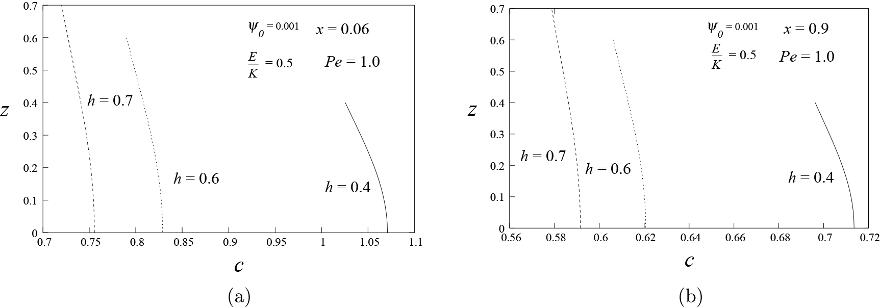
Distribution of concentration c with z at different cross sections (a) x = 0.06 and (b) x = 0.09.
Figure 3 shows the distribution of concentration c along normal direction z for various values of permeability of the poroelastic surface
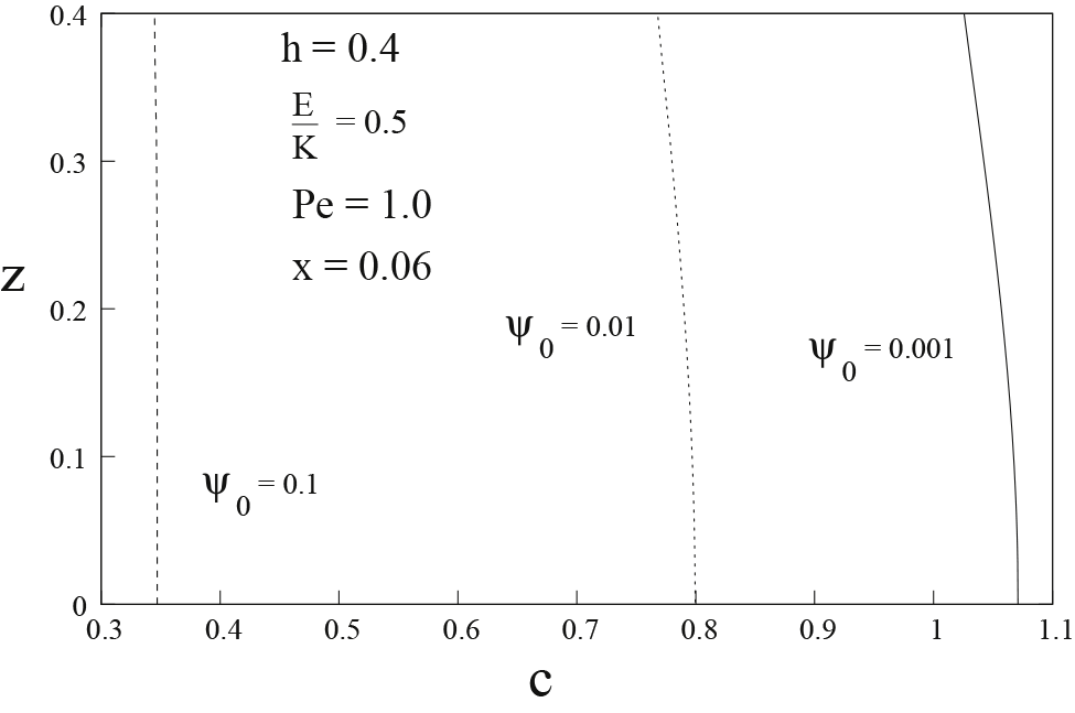
Distribution of concentration c with z for different values of
Effect of elastic parameter
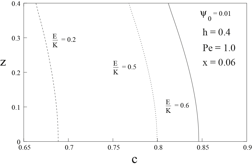
Distribution of concentration c with z for different values of
Figure 5 illustrates the influence of Peclet number
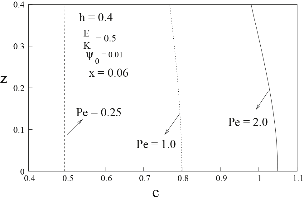
Distribution of concentration c with z for different values of Peclet number
Solute concentration at interface
Figure 6 represents axial distribution of solute concentration
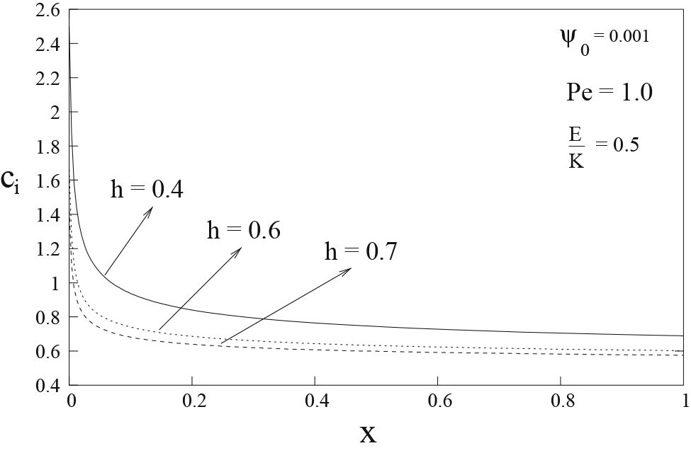
Distribution of concentration at the interface
Squeeze film pressure (p):
Axial distribution of squeeze film pressure p with x for various values of h is shown in Figure 7. The general pattern is that p increases as h decreases. It may be noted that when the gap between two articular surfaces decreases, there is a resistance to sideways flow and further, the viscosity of the fluid increases due to increase in concentration of HA in the film region. Because of these reasons, squeeze film pressure increases as the gap decreases.
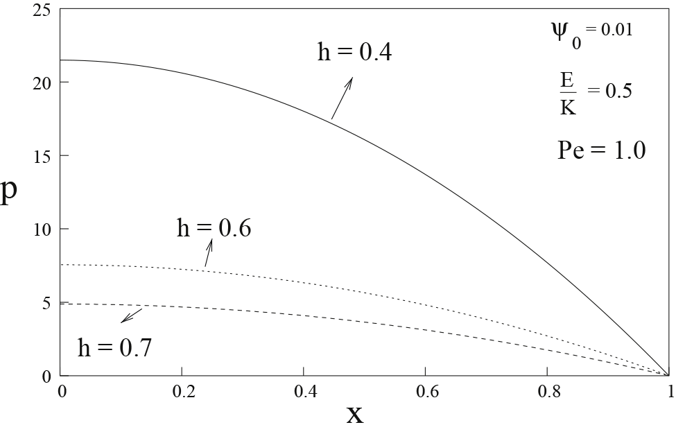
Distribution of pressure p with x for different values of h.
Figure 8 shows the effect of variation of permeability parameter
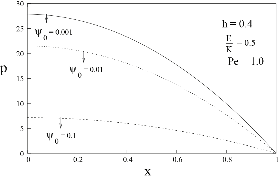
Distribution of pressure p with x for different values of
Figure 9 represents the distribution of squeeze film pressure p with x for various values of elastic parameter
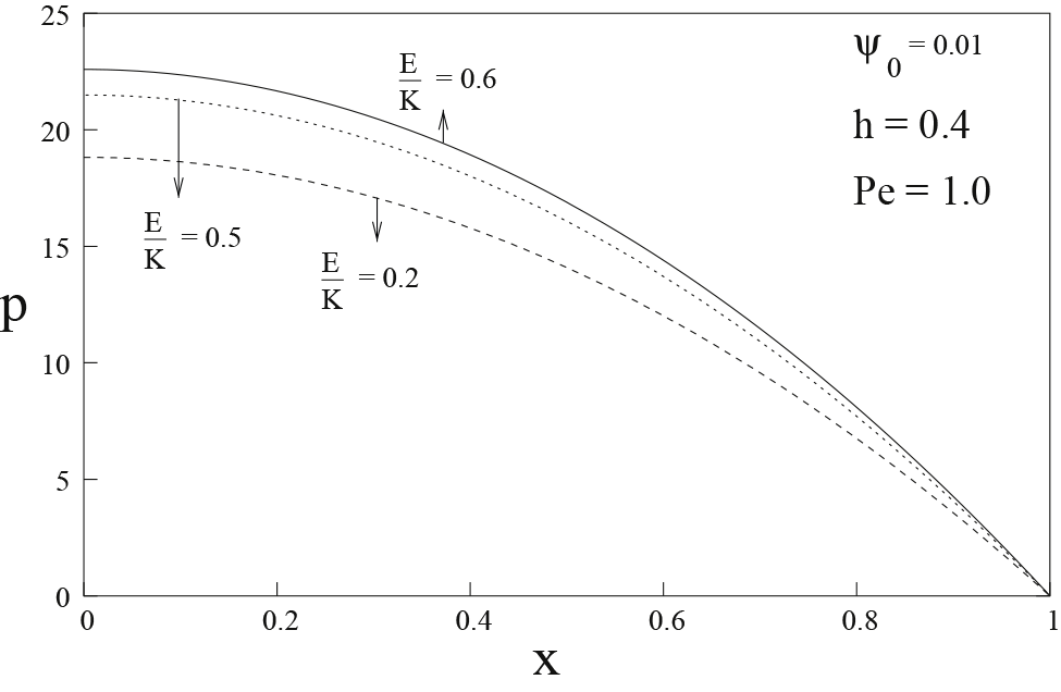
Distribution of pressure p with x for different values of
Load carrying capacity (W):
Variation of load carrying capacity W with film height h for different values of
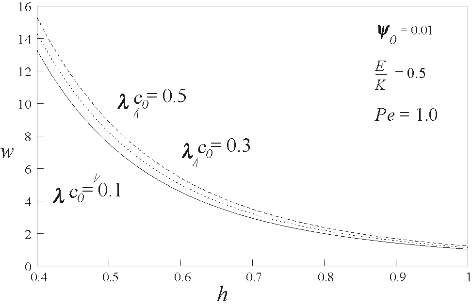
Variation of load carrying capacity W at various heights h for different values of
Figures 11 and 12 depict the variation of W with h for different values of
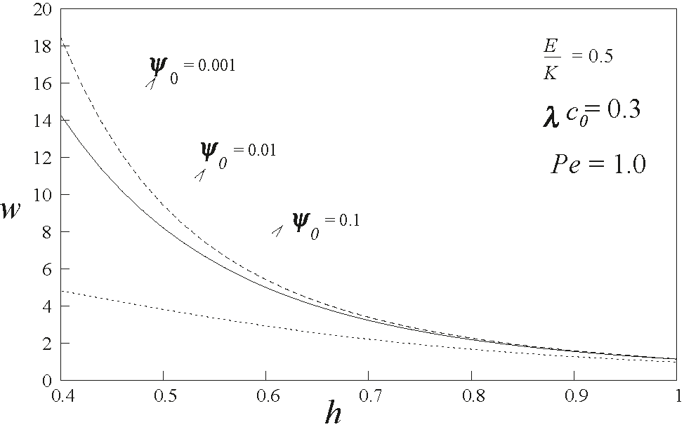
Variation of load carrying capacity W at various heights h for different values of
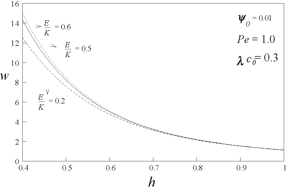
Variation of load carrying capacity W at various heights h for different values of
5 Conclusion
In this paper, a mathematical model has been proposed to study the squeeze film lubrication by taking into account the permeability, elasticity of the bearing surfaces and the viscosity variation of the lubricant due to change in the concentration of solute particles.
It is found that the squeeze film pressure and the load carrying capacity increase as the concentration of solute particle increases.
Further the concentration of solute particles, squeeze film pressure and load carrying capacity increase as the elastic parameter increases but they decrease with increase in the permeability.
The results obtained for various values of parameter h show a strong influence on the concentration of solute particles and the film pressure.
References
[1] N. M. Bujurke and R. B. Kudenatti, “An analysis of rough poroelastic bearings with reference to lubrication mechanism of synovial joints,” Appl. Math. Comput., vol. 178, pp. 309–320, 2006.10.1016/j.amc.2005.11.048Search in Google Scholar
[2] Peeyush Chandra, Mathematical Model for Synovial Joints – A Lubrication Biomechanical Study, PhD Thesis, IIT Kanpur, 1975.Search in Google Scholar
[3] P. A. Torzilli and V. C. Mow, “On the fundamental fluid transport mechanisms through normal and pathological articular cartilage during functon-II – The analysis, solution and conclusions,” J. Biomech., vol. 9, pp. 587–606, 1976.10.1016/0021-9290(76)90100-7Search in Google Scholar
[4] N. M. Bujurke, M. Jagadeeswar, and P. S. Hiremath, “Analysis of normal stress effects in a squeeze film porous bearing,” Wear, vol. 116, pp. 237–248, 1987.10.1016/0043-1648(87)90236-5Search in Google Scholar
[5] J. S. Hou, V. C. Mow, W. M. Lai, et al. “An analysis of the squeeze-film lubrication mechanism for articular cartilage,” J. Biomech., vol. 25, no. 3, pp. 247–259, 1992.10.1016/0021-9290(92)90024-USearch in Google Scholar
[6] P. N. Tandon, N. H. Bong, and Kushwaha Kiran, “A new model for synovial joint lubrication,” Int. J. Bio Med Comput. vol. 35, no. 2, pp. 125–140, 1994.10.1016/0020-7101(94)90062-0Search in Google Scholar
[7] N. M. Bujurke and R. B. Kudenatti, “Surface roughness effects on squeeze film poroelastic bearings,” Appl. Math. Comput., vol. 174, pp. 1181–1195, 2006.10.1016/j.amc.2005.06.007Search in Google Scholar
[8] P. S. Walker, D. Dowson, M. D. Longfield, and V. Wright, “Boosted lubrication in synovial joints by fluid entrapment and enrichment,” Ann. Rheum. Dis., vol. 27, pp. 512–522, 1968.10.1136/ard.27.6.512Search in Google Scholar
[9] A. S. Tannin, S. G. Nicholas, T. N. Quynhhoa, et al. “Boundary lubrication of articular cartilage – role of synovial fluid constituents,” Arthritis Rheumatol., vol. 56, no. 3, pp. 882–891, 2007.10.1002/art.22446Search in Google Scholar
[10] Richard Collins, “A model of lubricant gelling in synovial joints,” J. Appl. Math. Phys., vol. 33, pp. 93–123, 1982.10.1007/BF00948315Search in Google Scholar
[11] P. N. Tandon, P. Nirmala, T. S. Pal, et al. “Rheological study of lubricant gelling in synovial joints during articulation,” Appl. Math. Model., vol. 12, pp. 72–74, 1988.10.1016/0307-904X(88)90025-XSearch in Google Scholar
[12] M. Alshehri and S. K. Sharma, “Computational model for the generalised dispersion of synovial fluid,” IJACSA, vol. 8, no. 2, pp. 134–138, 2017.10.14569/IJACSA.2017.080218Search in Google Scholar
[13] P. Pustejovska, “Mathematical modeling of synovial fluids flow,” WDS'08 Proceedings of Contributed papers, Part III, pp. 32–37, 2008.Search in Google Scholar
[14] J. Hron, J. Malek, P. Pustejovska, et al. “On the modeling of the synovial fluid,” Adv. Tribol., pp. 1–12, 2010.10.1155/2010/104957Search in Google Scholar
[15] E. R. Morris, D. A. Rees, and E. J. Welsh, “Conformation and dynamic interactions in hyaluronate solutions,” J. Mol. Biol., vol. 138, no. 2, pp. 383–400, 1980.10.1016/0022-2836(80)90294-6Search in Google Scholar
[16] P. S. Walker and M. J. Erkman, “Metal-on-metal lubrication in artificial human joints,” Wear, vol. 21, pp. 377–392, 1972.10.1016/0043-1648(72)90011-7Search in Google Scholar
[17] O. Pinkus and B. Sternlicht, Theory of Hydrodynamic Lubrication, New York, McGraw-Hill, 1961.Search in Google Scholar
[18] N. B. Naduvinamani and G. K. Savitramma, Effect of Surface Roughness on the Squeeze Film Lubrication of Finite Poroelastic Partial Journal Bearing with Couple Stress Fluids: A Special Reference to Hip Joint Lubrication, ISRN Tribology, 2014. pp. 1–13.10.1155/2014/690147Search in Google Scholar
[19] J. Ferguson, J. A. Boyle, R. N. M. Mcsween, et al. “Observations on the flow properties of the synovial fluid from patients with rheumatoid arthritis,” Biorheology, vol. 5, no. 2, pp. 119–131, 1968.10.3233/BIR-1968-5204Search in Google Scholar
[20] R. Y. Hori and L. F. Mockros, “Indentation tests of human articular cartilage,” J. Biomech., vol. 9, no. 4, pp. 259–268, 1976.10.1016/0021-9290(76)90012-9Search in Google Scholar
[21] U. R. Shettigar, H. J. Prabhu, and D. N. Ghista, “Blood ultrafiltration: A design analysis.” Medi. Biol. Engg. Comput., vol. 15, no. 1, pp. 32–38, 1977.10.1007/BF02441572Search in Google Scholar
[22] J. Prakash and S. K. Vij, “Load capacity and time-height relations for squeeze films between porous plates,” Wear, vol. 24, pp. 309–322, 1973.10.1016/0043-1648(73)90161-0Search in Google Scholar
[23] T. J. Chung, Computational Fluid Dynamics, 2nd ed. Cambridge University press, 2010.10.1017/CBO9780511780066Search in Google Scholar
[24] Tamer Mahmoud Tamer, “Hyaluronan and synovial joint: function, distribution and healing,” Interdiscipl. Toxicol., vol. 6, no. 3, pp. 111–125, 2013.10.2478/intox-2013-0019Search in Google Scholar PubMed PubMed Central
[25] M. M. Temple-Wong, B. Hansen, M. Grissom, et al., “Effect of knee osteoarthritis on the boundary lubricating molecules and function of human synovial fluid,” Trans. Orthop. Res. Soc., vol. 35, pp. 340, 2010.Search in Google Scholar
[26] L. B. Dahl, I. M. Dahl, A. Engstrom-Laurent, et al. “Concentration and molecular weight of sodium hyaluronate in synovial fluid from patients with rheumatoid arthritis and other arthropathies,” Ann. Rheum. Dis, vol. 44, pp. 817–822, 1985.10.1136/ard.44.12.817Search in Google Scholar PubMed PubMed Central
[27] A. Maroudas, “Hyaluronic acid films,” Proc. Inst. Mech. Eng., vol. 181, pp. 122–124, 1967.10.1243/PIME_CONF_1966_181_214_02Search in Google Scholar
[28] P. S. Walker, J. Sikorski, D. Dowson, et al. “Behaviour of synovial fluid on surfaces of articular cartilage – A scanning electron microscope study,” Ann. Rheum. Dis., vol. 28, pp. 1–14, 1969.10.1136/ard.28.1.1Search in Google Scholar PubMed PubMed Central
© 2020 Walter de Gruyter GmbH, Berlin/Boston
Articles in the same Issue
- Frontmatter
- General
- Rapid Communication
- Pocket formula for alpha decay energies and half-lives of actinide nuclei
- Atomic, Molecular & Chemical Physics
- Rapid Communication
- On biological signaling
- Dynamical Systems & Nonlinear Phenomena
- Solution of the Riemann problem for an ideal polytropic dusty gas in magnetogasdynamics
- Gravitation & Cosmology
- Cosmological solutions in Hořava-Lifshitz scalar field theory
- Hydrodynamics
- Effect of concentration dependence of viscosity on squeeze film lubrication
- Solid State Physics & Materials Science
- Electronic band profiles and magneto-electronic properties of ternary XCu2P2 (X = Ca, Sr) compounds: insight from ab initio calculations
- Enhancing crystal quality and optical properties of GaN nanocrystals by tuning pH of the synthesis solution
- Experimental and computational studies on optical properties of a promising N-benzylideneaniline derivative for non-linear optical applications
- Studies of the Electronic, Optical, and Thermodynamic Properties for Metal-Doped LiH Crystals by First Principle Calculations