
Nonlinear Pull-in Instability of Rectangular Nanoplates Based on the Positive and Negative Second-Order Strain Gradient Theories with Various Edge Supports
-
A. Zabihi
 ,
K. Hosseini
,
K. Hosseini


Abstract
Based on the positive and negative second-order strain gradient theories along with Kirchhoff thin plate theory and von Kármán hypothesis, the pull-in instability of rectangular nanoplate is analytically investigated in the present article. For this purpose, governing models are extracted under intermolecular, electrostatic, hydrostatic, and thermal forces. The Galerkin method is formally exerted for converting the governing equation into an ordinary differential equation. Then, the homotopy analysis method is implemented as a well-designed technique to acquire the analytical approximations for analyzing the effects of disparate parameters on the nonlinear pull-in behavior. As an outcome, the impacts of nonlinear forces on nondimensional fundamental frequency, the voltage of pull-in, and softening and hardening effects are examined comparatively.
1 Introduction
Nanostructures such as nanobeams, nanotubes, and nanoplates have conspicuous importance for scholars because of their various applications in disparate systems; including nanoelectromechanical and microelectromechanical systems, nano biosensors, and nano actuators [1], [2]. It seems that the classical continuum theories are unable to consider the size effect in the mechanical analysis of nanostructures, as they do not contain any appropriate parameter; thus, some nonclassical continuum theories, such as nonlocal elasticity theory [3], [4], [5], [6], [7], [8], Gurtin–Murdoch elasticity continuum [9], couple stress theory [10], [11], and strain-driven and stress-driven nonlocal integral elasticity [12], [13], two-phase integral elasticity [14], [15], nonlocal strain gradient elasticity [16], [17], [18], [19], [20], [21], modified nonlocal strain gradient elasticity [22], and strain gradient theory (SGT) [23], [24], [25], [26], [27], [28], [29], [30], [31], [32], [33], have been proposed with the capability of considering the size effect.
One of the capable nonclassical continuum theories called SGT was first presented by Mindlin [23], [24]. The SGT has different forms and formulas; to exemplify, in the first-order SGT [23], only first strain gradients were calculated with five material length scales in the corresponding constitutive relations. In the second-order SGT [24], the second-order derivatives of strain were calculated in the strain energy density along with 16 material length scale parameters. Lam et al. [25] proposed successfully another form of SGT called the modified SGT, which has three material length scale parameters and considered strain energy density as a function of dilatation gradient, symmetric strain, deviatoric stretch gradient, and symmetric rotation gradient tensors. Scholars employed SGT to analyze the vibration of nanostructures. For instance, Thai et al. [26] applied the modified SGT to analyze free vibration and static bending of microplates. Torabi et al. [27], [28] implemented the 3-D SGT to analyze the free vibration of nanoplates.
Besides, Altan and Aifantis [29] and Aifantis [30] proposed the simplified SGT, which involves one length scale parameter. This simplified form of SGT has a positive and negative sign, which signifies softening and hardening behavior. The survey of the literature shows that several studies have been done with the help of this simplified form. To exemplify, Babu and Patel [31] studied linear bending, free vibration, and buckling of rectangular nanoplate based on the positive and negative SGT. Based on the positive and negative SGT, natural frequency and buckling load of Euler–Bernoulli beam/tubes were presented by Babu and Patel [32]. Babu and Patel [33] analyzed the transverse static loading of rectangular nanoplate using negative second-order SGT.
Considering another failure pattern of microstructures/nanostructures, when the movable electrode falls into the substrate one, because of the critical amounts of applied voltage, one of the prominent phenomena in the nanostructures called the pull-in instability occurs, and this phenomenon is not reversible. For the first time, the pull-in instability was informed experimentally by Taylor [34] and Nathanson et al. [35]. Other researchers worked on this phenomenon, for instance, Ansari et al. [36] analyzed the behavior of pull-in instability on rectangular nanoplates. Dynamic pull-in instability of a microbeam was studied by Yang et al. [37]. Gholami et al. [38] studied the pull-in instability of rectangular microplates based on the SGT. Pull-in instability of rectangular nanoplate was analyzed based on the modified couple stress theory by Wang et al. [39]. The interested reader is referred to [40], [41], [42], [43], [44], [45].
Generally, solution models for pull-in instability are divided into two categories of numerical and analytical solutions, and the second one is utilized in this article. It is transparent that the classical analytical methods are disabled to solve bouncing nonlinear ordinary differential equations (ODEs); hence, Liao [46] proposed a powerful solution strategy called the homotopy analysis method (HAM) to handle such nonlinear ODEs. Based on the application of HAM, other researchers utilized it in their articles, for example, Alipour et al. [47] employed HAM to analyze the nonlinear behavior of nanobeams. The HAM was applied via Samadani et al. [48] to scrutinize the pull-in instability of nanobeam.
It is invaluable to mention that in the present article two nonlinear forces including electrostatic and intermolecular ones are considered. In the intermolecular force portion, there are two forces such as the van der Waals (vdW) or the Casimir. When the space between two electrodes is less than the plasma wavelength of the ingredient material of surfaces, the vdW attraction is considered (typically <20 nm) [49]. On the other hand, the Casimir force [50], [51] is considered when space is larger than the aforementioned situation; thus, they do not exist simultaneously [47]. As a result, in this article, models are presented with considering the Casimir force. To procure mathematical modeling of hydrostatic and electrostatic actuation, some researches have been done [52], [53]. When the hydrostatic force is applied, the nanoplate is stable; nevertheless, the pull-in instability is occurred by applying electrostatic and intermolecular forces.
The main objective of this study is the geometrically nonlinear pull-in analysis of rectangular nanoplates based on the positive and negative second-order SGTs. The nonlinear governing equations based on the Kirchhoff thin plate theory, von Kármán nonlinear kinematic relation, and second-order SGTs are presented for the first time. The present study is organized as follows: In the following section, the governing equations are derived. In Section 3, the equations subjected to SSSS, CCCC, and CSCS boundary conditions (BCs) (clamped edges and simply supported are truncated to C and S) are converted to nondimensional equations and metamorphosed into ODEs through the Galerkin method (GM). In Section 4, the HAM is used to procure analytical approximate solutions of governing models. In Section 5, the effects of intermolecular, electrostatic, hydrostatic, and thermal forces, along with nonlinear fundamental frequency, the pull-in voltage, softening, and hardening impacts, are investigated. In Section 6, the main achievements of the article are given.
2 Model Description
2.1 Second-Order SGT
Generally, the second-order SGT has two forms of positive and negative coefficient. The main difference between them is that the positive form evinces softening effect, albeit the negative equivalent represents the hardening effect [29], [30], [31], [32], [33]. The positive and negative second-order SGTs are presented in the following-40pt form:
where
2.2 Kirchhoff Plate Theory
Based on Kirchhoff’s theory, the displacement of plate u, v and w along with x, y, and z directions can be shown as follows:
where w is the transverse displacement of the plate. Based on Kirchhoff’s theory, deduced from the classical elasticity formulation of Saint-Venant problem [54], [55], [56], and von Kármán hypothesis, the strains in the classical rectangular plate can be expressed as
The geometrically linear relations can be obtained by removing
where
where the thickness of the nanoplate is h. Thus, by substituting (4) in the aforementioned formulas, the force and moment resultants for the second-order SGT are procured relatively in terms of transverse displacement
where
where T, W, U, and K signify time, work of external forces, strain energy, and kinetic energy, respectively. First, the variation of strain energy is displayed as
where S points out the area.
Second, the variation of the work of external loads has the following form:
where the terms
where h and α indicate the thickness of the nanoplate and the coefficient of thermal expansion [57].
Lastly, by considering the integration by parts in the time domain, the variation of the kinetic energy is
where
Equations (10) to (12) are substituted in (9), thereupon the governing equation for rectangular nanoplates is obtained in this form:
where
Note that the governing equation is converted to the classical model by setting l = 0.
3 Mathematical Modeling
Schematic of the rectangular nanoplate with length la and width lb, including a pair of parallel electrodes with the distance g, is given in Figure 1. The upper movable electrode is assumed to be under the impact of electrostatic, intermolecular, hydrostatic, and thermal forces.
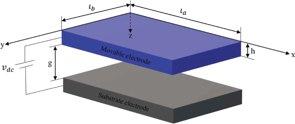
Schematic of a NEMS rectangular nanoplates.
The electrostatic force per unit area can be expressed as follows [60]:
where
The Casimir force relatively per unit area of the rectangular plate has the following formula [50], [51]:
where the Plank’s constant is
where Fh stands for the hydrostatic actuation.
| Boundary condition | |||
|---|---|---|---|
| Clamped | Classic | ||
| Nonclassic | |||
| Simply supported | Classic | ||
| Nonclassic |
In this attitude, (15) and (16) are substituted in (17) and inserted in (14), so the governing equations of second-order SGT are procured:
The BCs of rectangular isotropic Kirchhoff nanoplate are presented in Table 1. The BCs are presented as the classical and nonclassical ones.
These nondimensional variables are applied comparatively:
and Taylor expansion is employed as follows:
Therefore, the nondimensional form of the governing equation is achieved:
Now, GM is used due to altering (22) to ODE. The related formula is used:
where
are the first eigenmode of nanoplate.
The
For instance, the parameters M and
4 Applying the HAM
To apply the HAM, the following transformation is used:
Then, (25) is turned into the following equation:
where B signifies the initial amplitude; furthermore, the frequency
According to the HAM, the zeroth-order deformation equation is considered as follows:
where ℒ, q, and 𝒩 are the linear operator, embedding parameter, and the nonlinear operator, respectively. The linear and nonlinear operators are defined as follows:
The solution
Relatively, differentiating zeroth-order deformation (29) with respect to q results in
By substituting
For removing the secular terms, coefficient of
and
5 Results and Discussion
The geometry of the structure and material properties are presented in Table 2 [36]. To validate the results of this research, the natural frequencies of the nanoplate analyzed through Babu and Patel [31] are compared in Table 3. Otherwise stated, the parameters are considered as μ = 0.1, θ = 300, and initial amplitude B = 0.1.
In Figure 2, the nondimensional deflection is derived by the HAM and compared to that obtained through the Runge–Kutta method verifying complete arrangement. Based on the graphs, negative second-order SGT is plotted in different BCs such as CCCC, CSCS, and SSSS considering geometrical nonlinear hypothesis.
Material properties and geometrical of the rectangular nanoplate [36].
| Parameter | Value |
| Young modulus (Al alloy) | 68.5 GPa |
| Poisson ratio (Al alloy) | 0.35 |
| Coefficient of thermal expansion | −2.6 × 10⁻⁶ 1/°C |
| Thickness (h) | 21 nm |
| Length | 30 h |
| Gap | 1.2 h |
Comparison of the natural frequencies of nanoplates based on the second-order SGT with the results of Babu and Patel [31] (SSSS).
| Second-order SGT | Length scale | ||||
|---|---|---|---|---|---|
| 0 | 0.02 | 0.05 | 0.1 | ||
| Positive | Babu and Patel [31] | 19.7205 | 19.6432 | 19.2328 | – |
| Present study | 19.7205 | 19.6425 | 19.2277 | 17.6672 | |
| Negative | Babu and Patel [31] | 19.7205 | 19.7976 | 20.1971 | 21.5632 |
| Present study | 19.7205 | 19.7982 | 20.2012 | 21.5792 | |
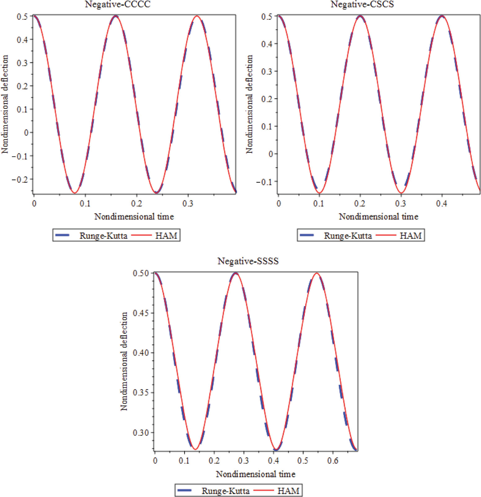
The Runge–Kutta method against HAM results on negative second-order SGT (μ = 0.04, Vdc = 2, B = 0.5).
The variations of nondimensional deflection against the nondimensional time are disclosed in Figure 3. Certainly, the movable nanoplate deflects into the substrate one, when the pull-in occurs. According to Table 4, the CCCC has a higher pull-in voltage than other BCs. Also, in all of BCs, the positive theory has lower pull-in voltage than the negative one. Based on Table 4, one can also find that by considering the geometrical nonlinear terms the range of pull-in voltage changed lower than the geometrical linear situation.
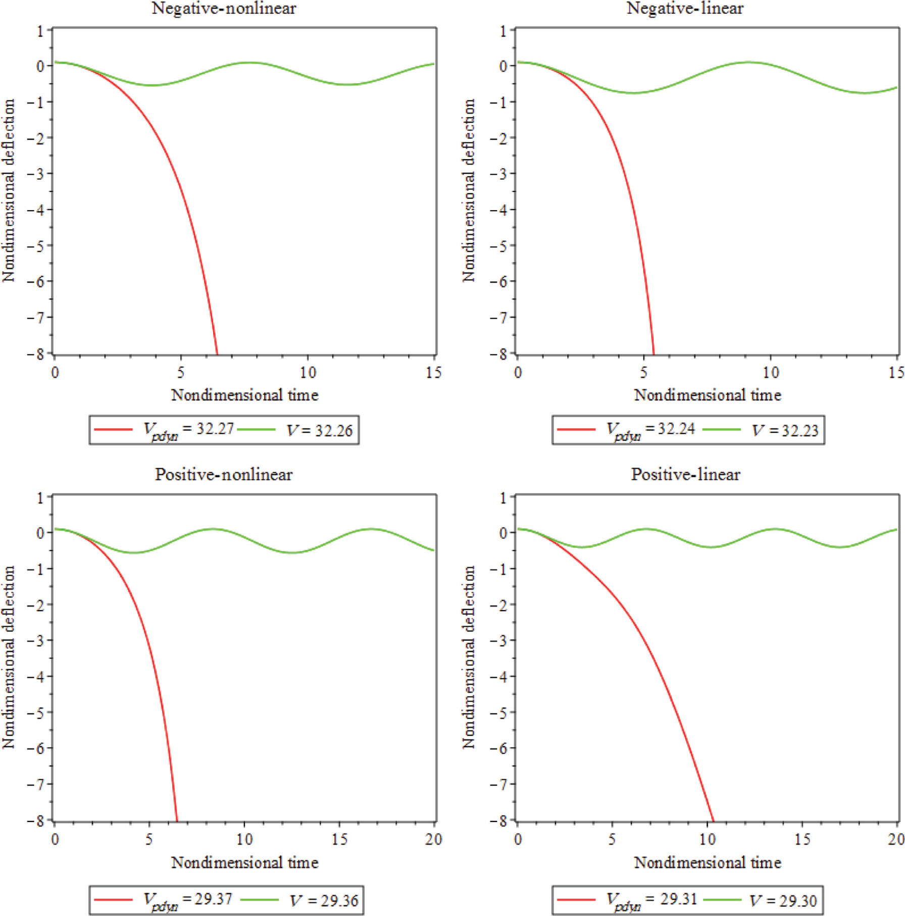
Centerpoint deflection of rectangular nanoplates considering geometrical nonlinear and linear terms in CCCC BC.
Dynamic pull-in voltage of the rectangular nanoplate.
| Second-order SGT | Geometrical | Length scale | CCCC | CSCS | SSSS |
|---|---|---|---|---|---|
| Negative | Nonlinear | 0 | 30.86 | 24.55 | 16.37 |
| 0.03 | 31.66 | 25.05 | 16.52 | ||
| 0.06 | 33.96 | 26.50 | 16.94 | ||
| 0.10 | 38.87 | 29.65 | 17.89 | ||
| Linear | 0 | 30.81 | 24.50 | 16.32 | |
| 0.03 | 31.62 | 25.01 | 16.46 | ||
| 0.06 | 33.94 | 26.47 | 16.89 | ||
| 0.10 | 38.88 | 29.66 | 17.86 | ||
| Positive | Nonlinear | 0 | 30.86 | 24.55 | 16.37 |
| 0.03 | 30.03 | 24.03 | 16.23 | ||
| 0.06 | 27.40 | 22.43 | 15.79 | ||
| 0.10 | 19.83 | 18.05 | 14.70 | ||
| Linear | 0 | 30.81 | 24.50 | 16.32 | |
| 0.03 | 29.98 | 23.98 | 16.17 | ||
| 0.06 | 27.33 | 22.36 | 15.73 | ||
| 0.10 | 19.66 | 17.92 | 14.61 |
The nondimensional fundamental frequency with respect to β is displayed in Figure 4 in order to show the size dependency based on the positive and negative second-order SGTs. It is clear that the nondimensional fundamental frequency reduces by increasing the λ; consequently, the pull-in instability delayed as λ is increased. On the other side, the pull-in instability occurs at a lower voltage by decreasing the λ. Moreover, this situation is free from nonclassical continuum theories and BCs.
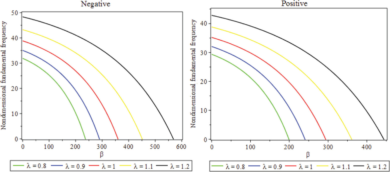
Impact of size dependency on nondimensional fundamental frequency against electrostatic force considering CCCC BC.
In Figure 5, the deviations of the nondimensional fundamental frequencies against β are revealed for dissimilar values of the nondimensional length scale parameters (μ) in order to show the softening and hardening behavior. It can be inferred that through intensifying μ the nondimensional fundamental frequency abates for positive second-order SGT and enhances for the negative one relatively. Likewise, the softening and hardening behaviors are displayed based on the positive and negative second-order SGTs with considering geometrical nonlinearity.
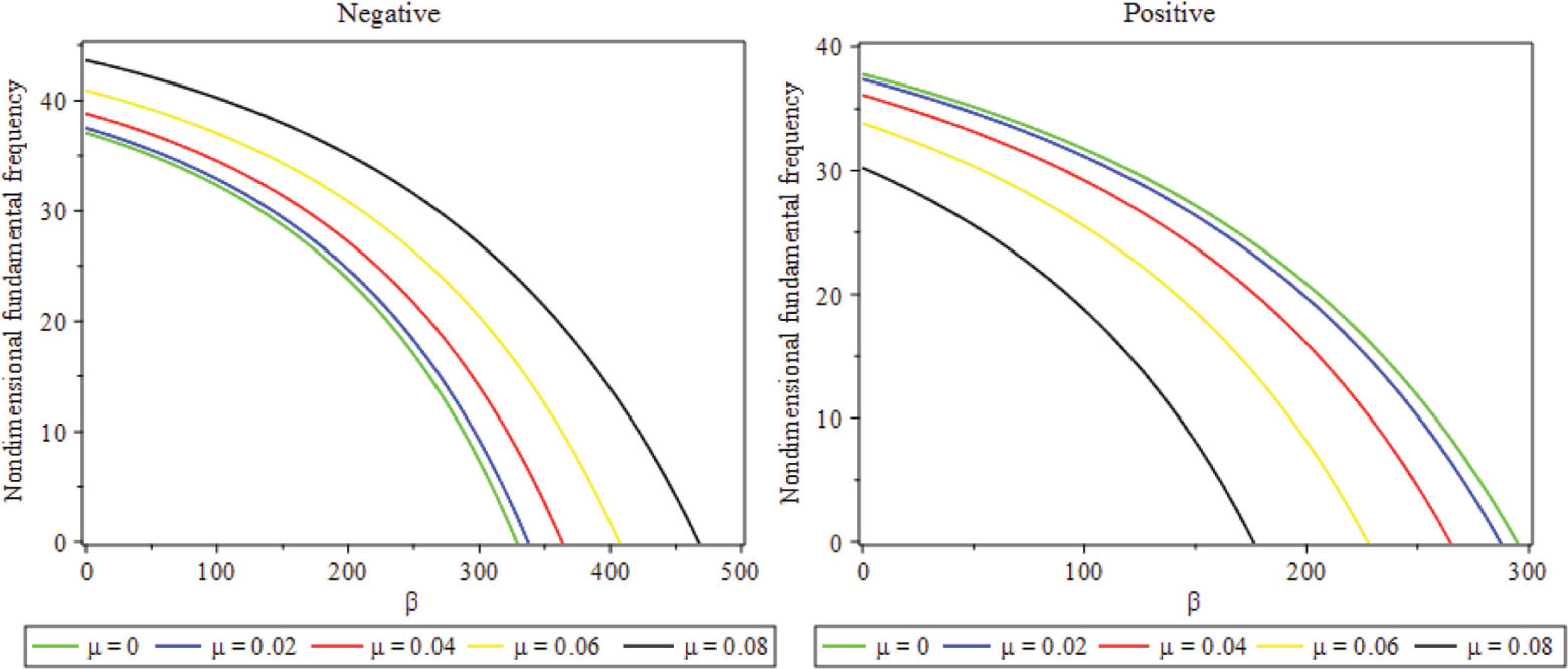
Impact of the parameter μ on the nondimensional fundamental frequency against nondimensional electrostatic actuation considering CCCC BC.
The differences of the nondimensional fundamental frequencies against nondimensional hydrostatic pressure parameters on behalf of dissimilar values of μ are exhibited in Figure 6 with considering CCCC BC. One can find that via rising Nhs, the fundamental frequency decreases comparatively, and it is the prime characteristic of hydrostatic pressure.
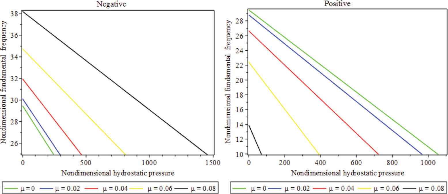
Outcome of parameter μ on nondimensional fundamental frequency versus nondimensional hydrostatic pressure considering CCCC BC
In Figure 7, the variations of the nondimensional fundamental frequencies versus NT are presented for disparate values of μ. It can be concluded that by increasing NT the nondimensional fundamental frequency enlarges, thereupon the gist of thermal actuation is sensible.
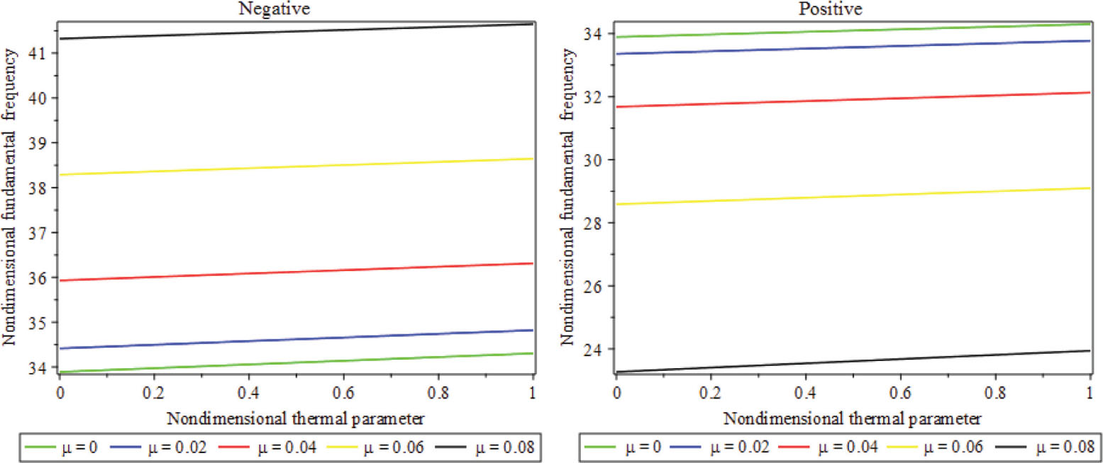
Influence of parameter μ on nondimensional fundamental frequency against nondimensional thermal actuation considering CCCC BC
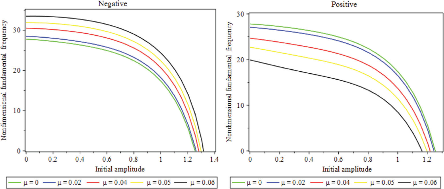
Consequence of parameter μ on nondimensional fundamental frequency versus initial amplitude considering CCCC BC
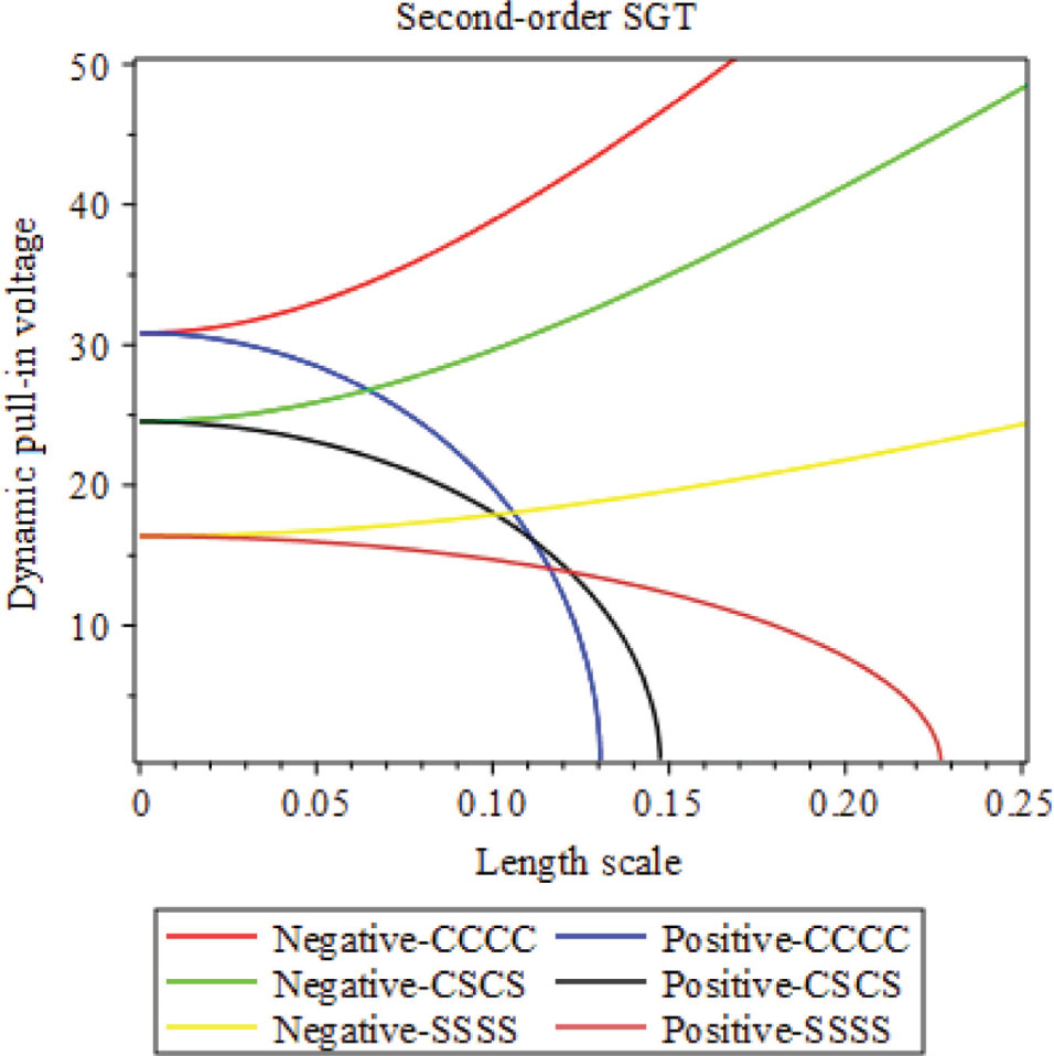
Dynamic pull-in voltage against length scale.
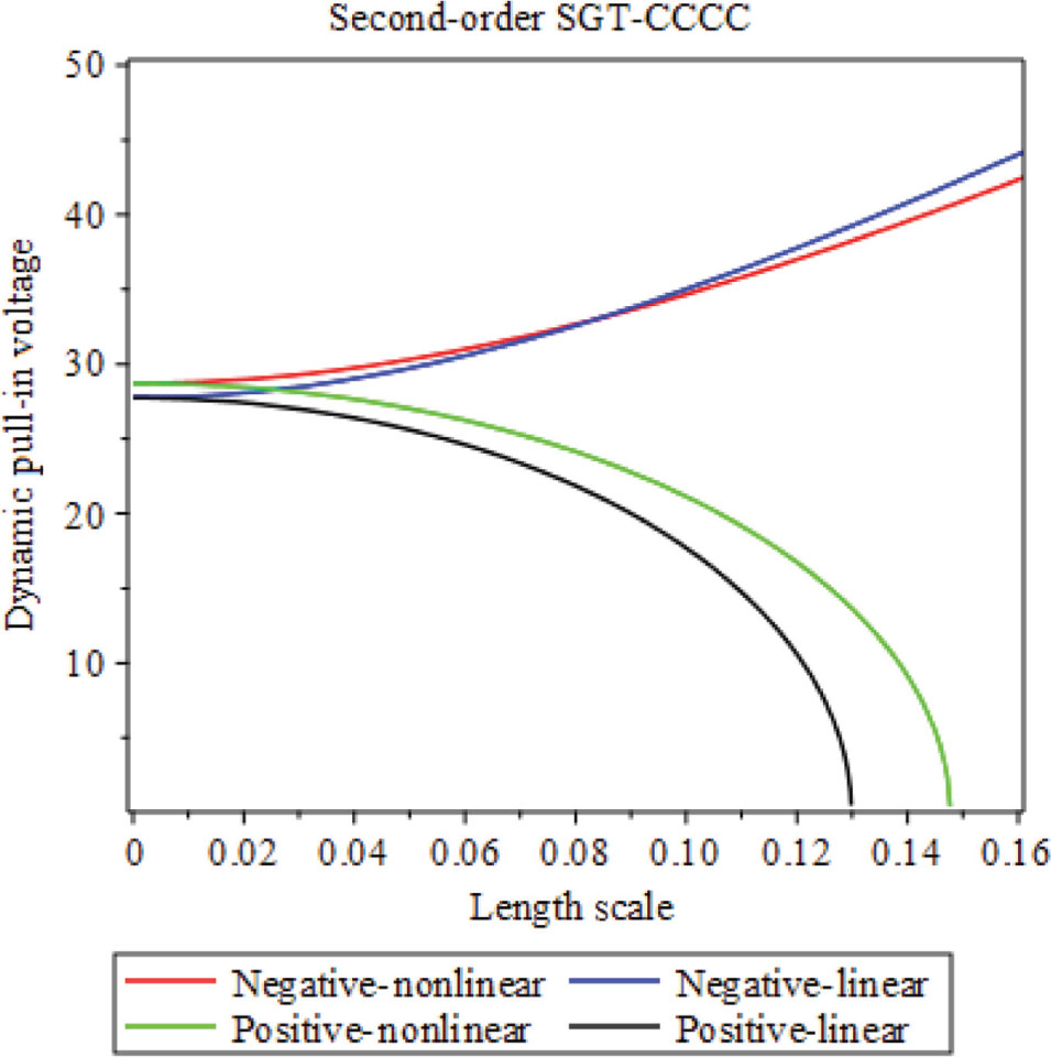
Dynamic pull-in voltage against length scale in CCCC BC
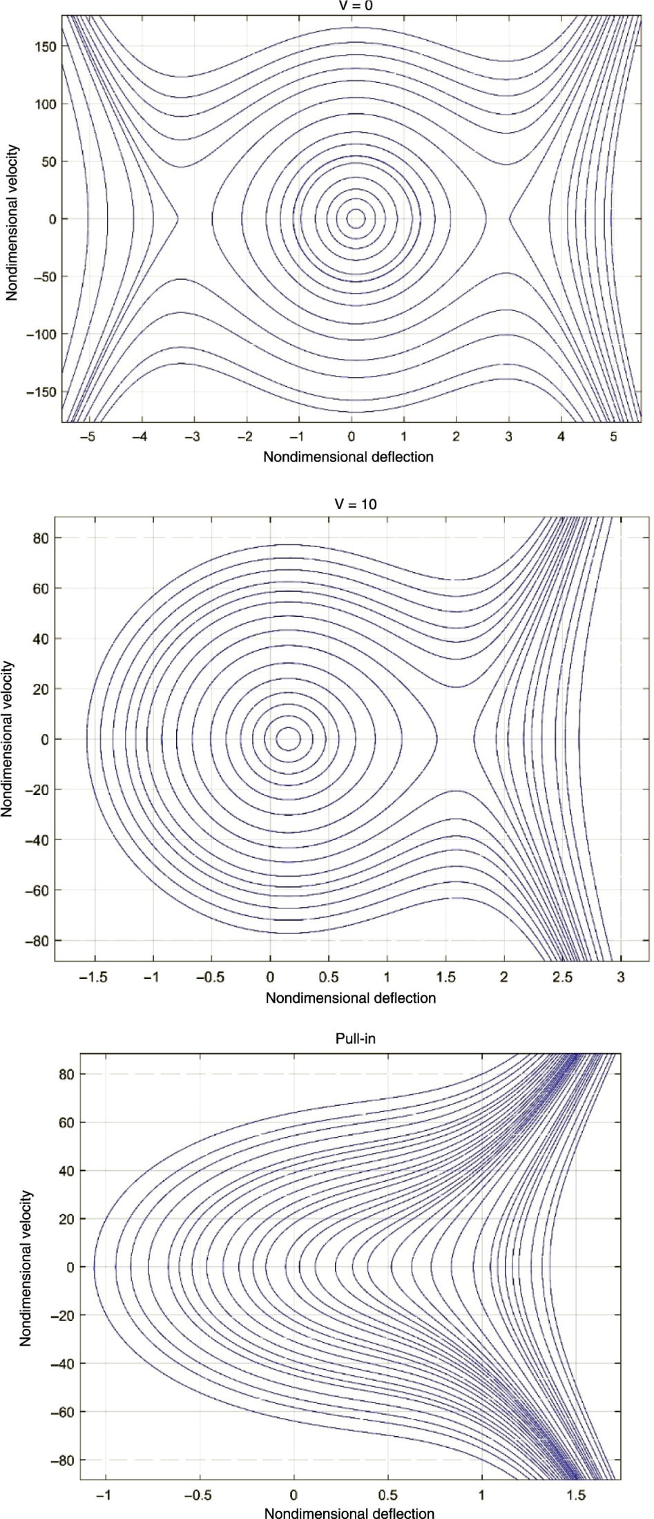
Phase diagram based on negative second-order SGT in CCCC BC.
The variations of the nondimensional fundamental frequency against initial amplitude are presented in Figure 8 for disparate values of μ. It is pellucid that by enhancing B the nonlinear frequency declines, and this attitude is free from BCs and the type of second-order SGT.
In Figure 9 dynamic pull-in voltage against length scale is presented based on the positive and negative second-order SGTs in different BCs and considering geometrical nonlinear terms. One can find that by increasing the length scale parameter the hardening behavior has occurred in negative theory, but the softening behavior is visible in a positive one.
Dynamic pull-in voltage against length scale is depicted based on the positive and negative second-order SGTs with considering geometrical linear and nonlinear in CCCC BC, as shown in Figure 10. It can be concluded that the dynamic pull-in voltage is decreased in positive theory by increasing the length scale parameter; however, it is increased in the negative one.
To show the pull-in nature and its destructive behavior on the nanosensor, the nondimensional velocity
6 Conclusion
In this article, the pull-in instability of rectangular nanoplates subjected to the electrostatic, hydrostatic, intermolecular, and thermal forces was analyzed based on the positive and negative second-order SGTs. Additionally, the von Kármán hypothesis was considered to apply geometrical nonlinearity, and Hamilton’s principle was employed to obtain the nonlinear governing equation. In this respect, GM was used for converting the governing equation to ODE in the time domain, with employing appropriate shape functions for different BCs. Then, the HAM was implemented as an analytical solution methodology. For analyzing the issue, various analytical results were reported. The results expose the folllowing:
In negative second-order SGT, through increasing length scale parameter, the nondimensional fundamental frequency enhances. Conversely, in positive second-order SGT, the nondimensional fundamental frequency subsides via intensifying the length scale parameter.
The nondimensional pull-in voltage and fundamental frequency are increased by increasing the nanoplates aspect ratio.
By escalating hydrostatic pressure, the nondimensional fundamental frequency decreases, but it is increased by intensifying the thermal load.
The softening and hardening effects are discovered through mechanical behavior in agreement with the positive and negative second-order SGTs.
Appendix
Parameters of positive second-order SGT in CCCC BC considering geometrical nonlinearity:
Parameters of negative second-order SGT in CCCC BC considering geometrical nonlinearity:
References
[1] M. Trabelssi, S. El-Borgi, L. L. Ke, and J. N. Reddy, Compos. Struct. 176, 736 (2017).10.1016/j.compstruct.2017.06.010Search in Google Scholar
[2] R. C. Batra, M. Porfiri, and D. Spinello, J. Sound Vib. 309, 600 (2008).10.1016/j.jsv.2007.07.030Search in Google Scholar
[3] A. C. Eringen and D. G. B. Edelen, Int. J. Eng. Sci. 10, 233 (1972).10.1016/0020-7225(72)90039-0Search in Google Scholar
[4] A. C. Eringen, J. Appl. Phys. 54, 4703 (1983).10.1063/1.332803Search in Google Scholar
[5] M. Bastami and B. Behjat, J. Braz. Soc. Mech. Sci. 40, 281 (2018).10.1007/s40430-018-1196-3Search in Google Scholar
[6] R. Ansari, J. Torabi, and M. Faghih Shojaei, Mech. Adv. Matl. Struct. 25, 500 (2018).10.1080/15376494.2017.1285457Search in Google Scholar
[7] M. Karimi, H. R. Mirdamadi, and A. R. Shahidi, J. Braz. Soc. Mech. Sci. 39, 1391 (2017).10.1007/s40430-016-0595-6Search in Google Scholar
[8] C. M. Wang, Y. Y. Zhang, and X. Q. He, Nanotechnology 18, 10 (2007).10.1088/0957-4484/18/10/105401Search in Google Scholar
[9] M. E. Gurtin and A. I. Murdock, Arch. Ration. Mech. An. 57, 291 (1975).10.1007/BF00261375Search in Google Scholar
[10] F. A. C. M. Yang, A. C. M. Chong, D. C. C. Lam, and P. Tong, Int. J. Solids Struct. 39, 2731 (2002).10.1016/S0020-7683(02)00152-XSearch in Google Scholar
[11] J. Kim, K. K. Zur, and J. N. Reddy, Compos. Struct. 209, 879 (2019).10.1016/j.compstruct.2018.11.023Search in Google Scholar
[12] M. Faraji Oskouie, R. Ansari, and H. Rouhi, Acta. Mech. Sin. 34, 871 (2018).10.1007/s10409-018-0757-0Search in Google Scholar
[13] R. Barretta, S. Ali Faghidian, and R. Luciano, Mech. Adv. Matl. Struct. 26, 15 (2019).10.1080/15376494.2018.1516253Search in Google Scholar
[14] A. Apuzzo, R. Barretta, F. Fabbrocino, S. Ali Faghidian, R. Luciano, et al., J. Appl. Comput. Mech. 5, 402 (2019).Search in Google Scholar
[15] R. Barretta, F. Fabbrocino, R. Luciano, and F. Marotti de Sciarra, Physica E 97, 13 (2018).10.1016/j.physe.2017.09.026Search in Google Scholar
[16] C. W. Lim, G. Zhang, and J. N. Reddy, J. Mech. Phys. Solids. 78, 298 (2015).10.1016/j.jmps.2015.02.001Search in Google Scholar
[17] H. Tang, L. Li, Y. Hu, W. Meng, and K. Duan, Thin Wall. Struct. 137, 377 (2019).10.1016/j.tws.2019.01.027Search in Google Scholar
[18] L. Lu, X. Guo, and J. Zhao, Appl. Math. Model. 68, 583 (2019).10.1016/j.apm.2018.11.023Search in Google Scholar
[19] R. Barretta, S. Ali Faghidian, F. Marotti de Sciarra, R. Penna, and F. P. Pinnola, Compos. Struct. 233, 111550 (2020).10.1016/j.compstruct.2019.111550Search in Google Scholar
[20] M. R. Barati, J. Braz. Soc. Mech. Sci. 39, 4335 (2017).10.1007/s40430-017-0890-xSearch in Google Scholar
[21] L. Li, L. Xiaobai, and H. Yujin Hu, Int J Eng Sci 102, 77 (2016).10.1016/j.ijengsci.2016.02.010Search in Google Scholar
[22] A. Apuzzo, R. Barretta, S. A. Faghidian, R. Luciano, and F. Marotti de Sciarro, Int. J. Eng. Sci. 133, 99 (2018).10.1016/j.ijengsci.2018.09.002Search in Google Scholar
[23] R. D. Mindlin, Arch. Ration. Mech. An. 16, 51 (1964).10.1007/BF00248490Search in Google Scholar
[24] R. D. Mindlin, Int. J. Solid. Struct. 1, 417 (1965).10.1016/0020-7683(65)90006-5Search in Google Scholar
[25] D. C. C. Lam, F. Yang, A. C. M. Chong, J. Wang, and P. Tong, J. Mech. Phys. Solids. 51, 1477 (2003).10.1016/S0022-5096(03)00053-XSearch in Google Scholar
[26] C. H. Thai, A. J. M. Ferreira, T. Rabczuk, and H. Nguyen-Xuan, Eur. J. Phys. A Solids 72, 521 (2018).10.1016/j.euromechsol.2018.07.012Search in Google Scholar
[27] J. Torabi, R. Ansari, and M. Darvizeh, Comput. Method Appl. M. 344, 1124 (2019).10.1016/j.cma.2018.09.016Search in Google Scholar
[28] J. Torabi, R. Ansari, and M. Darvizeh, Compos. Struct. 205, 69 (2018).10.1016/j.compstruct.2018.08.070Search in Google Scholar
[29] S. B. Altan and E. C. Aifantis, Scripta Metall. Mater. 26, 319 (1992).10.1016/0956-716X(92)90194-JSearch in Google Scholar
[30] E. C. Aifantis, J. Mech. Behav. Mater. 5, 355 (1994).10.1515/JMBM.1994.5.3.355Search in Google Scholar
[31] B. Babu and B. P. Patel, Compos. Part B 168, 302 (2019).10.1016/j.compositesb.2018.12.066Search in Google Scholar
[32] B. Babu and B. P. Patel, Mech. Adv. Matl. Struct. 26, 15 (2019).10.1080/15376494.2018.1516253Search in Google Scholar
[33] B. Babu and B. P. Patel, Eur. J. Mech. A Solids 73, 101 (2019).10.1016/j.euromechsol.2018.07.007Search in Google Scholar
[34] G. Taylor, Proc. R. Soc. Lon. Ser.-A 306, 423 (1968).10.1098/rspa.1968.0159Search in Google Scholar
[35] H. C. Nathanson, W. E. Newell, R. A. Wickstorm, and J. R. Davis, IEE Trans. Elec. Devices 14, 3 (1967).10.1109/T-ED.1967.15886Search in Google Scholar
[36] R. Ansari, V. Mohammadi, M. Faghihi Shojaei, R. Gholami, and M. A. Darabi, Int. J. Nonlin. Mech. 67, 16 (2014).10.1016/j.ijnonlinmec.2014.05.012Search in Google Scholar
[37] L. Yang, F. Fang, J. S. Peng, and J. Yang, Int. J. Struct. Stab. Dy. 17, 10 (2017).10.1142/S0219455417501176Search in Google Scholar
[38] R. Gholami, R. Ansari, and H. Rouhi, Int. J. Struct. Stab. Dy. 19, 2 (2019).10.1142/S021945541950007XSearch in Google Scholar
[39] K. F. Wang, T. Kitamura, and B. Wang, Int. J. Mech. Sci. 99, 288 (2015).10.1016/j.ijmecsci.2015.05.006Search in Google Scholar
[40] K. F. Wang, B. Wang, and C. Zhang, Acta. Mech. 228, 129 (2017).10.1007/s00707-016-1701-7Search in Google Scholar
[41] A. Zabihi, R. Ansari, J. Torabi, F. Samadani, and K. Hosseini, Mater. Res. Exp. 6, 0950b3 (2019).10.1088/2053-1591/ab31bcSearch in Google Scholar
[42] F. Samadani, R. Ansari, K. Hosseini, and A. Zabihi, Commun. Theor. Phys. 71, 349 (2019).10.1088/0253-6102/71/3/349Search in Google Scholar
[43] I. Karimipour, Y. T. Beni, A. Koochi, and M. Abadyan, J. Braz. Soc. Mech. Sci. 38, 1779 (2016).10.1007/s40430-015-0385-6Search in Google Scholar
[44] D. J. Hasanyan, R. C. Batra, and S. Harutyunyan, J. Therm. Stresses 31, 1006 (2008).10.1080/01495730802250714Search in Google Scholar
[45] M. Moghimi Zand and M. T. Ahmadian, Mech. Res. Comm. 36, 851 (2009).10.1016/j.mechrescom.2009.03.004Search in Google Scholar
[46] S. Liao, Homotopy Analysis Method in Nonlinear Differential Equations, Springer, Beijing, China 2012.10.1007/978-3-642-25132-0Search in Google Scholar
[47] A. Alipour, M. Moghimi Z, and H. Daneshpajooh, Sci. Iran F 22, 1322 (2015).Search in Google Scholar
[48] F. Samadani, P. Moradweysi, R. Ansari, K. Hosseini, and A. Darvizeh, Z. Naturforsch. A 72, 1093 (2017).10.1515/zna-2017-0174Search in Google Scholar
[49] A. Gusso and G. J. Delben, J. Phys. D Appl. Phys. 41, 17 (2008).10.1088/0022-3727/41/17/175405Search in Google Scholar
[50] S. K. Lamoreaux, Phys. Rev. Lett. 78, 1 (1997).10.1103/PhysRevLett.78.1Search in Google Scholar
[51] M. J. Sparnaay, Physica 24, 751 (1958).10.1016/S0031-8914(58)80090-7Search in Google Scholar
[52] A. Nabian, G. Rezazadeh, M. Haddad-derafshi, and A. Tahmasebi, Microsyst. Technol. 14, 235 (2008).10.1007/s00542-007-0425-ySearch in Google Scholar
[53] R. Ansari, R. Gholami, V. Mohammadi, and M. Faghihi Shojaei, J. Comput. Nonlin. Dyn. 8, 021015-1 (2013).10.1115/1.4007358Search in Google Scholar
[54] R. Barretta, Acta. Mech. 224, 2955 (2013).10.1007/s00707-013-0912-4Search in Google Scholar
[55] R. Barretta, Acta. Mech. 225, 2075 (2014).10.1007/s00707-013-1085-xSearch in Google Scholar
[56] S. Ali Faghidian, Int. J. Mech. Sci. 111, 65 (2016).10.1016/j.ijmecsci.2016.04.003Search in Google Scholar
[57] A. D. Kovalenko, Strength Mater. 3, 1134 (1971).10.1007/BF01527541Search in Google Scholar
[58] X. J. Xu, X. C. Wang, M. L. Zheng, and Z. Ma, Compos. Struct. 160, 366 (2017).10.1016/j.compstruct.2016.10.038Search in Google Scholar
[59] Y. M. Yue, C. Q. Ru, and K. Y. Xu, Int. J. Nonlin. Mech. 88, 67 (2017).10.1016/j.ijnonlinmec.2016.10.013Search in Google Scholar
[60] R. C. Batra, M. Porfiri, and D. Spinello, Int. J. Solid Struct. 45, 3558 (2008).10.1016/j.ijsolstr.2008.02.019Search in Google Scholar
[61] K. Rashvand, G. Rezazadeh, and H. Madinei, Int. J. Eng. 27, 375 (2014).Search in Google Scholar
© 2020 Walter de Gruyter GmbH, Berlin/Boston
Articles in the same Issue
- Frontmatter
- Atomic, Molecular & Chemical Physics
- The Reaction and Microscopic Electron Properties from Dynamic Evolutions of Condensed-Phase RDX Under Shock Loading
- Trace Hydrogen Sulphide Gas Sensor Based on Cu/rGO Membrane-Coated Photonic Crystal Fibre Michelson Interferometer
- Dynamical Systems & Nonlinear Phenomena
- A General Viscous Model for Some Aspects of Tropical Cyclonic Winds
- Nonlinear Pull-in Instability of Rectangular Nanoplates Based on the Positive and Negative Second-Order Strain Gradient Theories with Various Edge Supports
- Hydrodynamics
- On the Heat Flow Through a Porous Tube Filled with Incompressible Viscous Fluid
- Effect of Magnetic Field on the Unsteady Boundary Layer Flows Induced by an Impulsive Motion of a Plane Surface
- Solid State Physics & Materials Science
- Facile Combustion Synthesis of (Y,Pr)2O3 Red Phosphor: Study of Luminescence Dependence on Dopant Concentration and Enhancement by the Effect of Co-dopant
- Size-Dependent Ultrasonic and Thermophysical Properties of Indium Phosphide Nanowires