Investigation of the Finite Size Properties of the Ising Model Under Various Boundary Conditions

1 Introduction

Finite-size scaling has been developed intensively during the last few decades [1], [2], [3], [4], and it has become a standard tool in the studies of critical systems. As soon as one has a finite system, one must consider the question of boundary conditions on the outer surfaces or “walls” of the system. As the boundary conditions affect only a small part of the system, we expect that as long as the system is finite we can observe some differences if we choose different boundary conditions, but as soon as we take the thermodynamic limit, these differences become irrelevant. The boundary conditions dependence of the finite-scaling functions is an interesting subject in condensed matter physics and statistical mechanics. Analytical results about the effect of boundary conditions on the finite-size scaling functions are scarce [5], [6], [7], [8]. To understand the effects of boundary conditions on finite-size scaling, it is valuable to study model systems, especially those that have exact results.

The Ising model [9], [10], [11] is a well-known and well-studied model for describing the magnetic system, where a spin variable that takes two possible values lives on each lattice site, which interact only with its nearest neighbours of magnetism. Although the magnetic and thermodynamic properties of the Ising model were investigated for an arbitrary lattice size N, usual focus of analysis has been in the thermodynamic limit.

The present article will be devoted to the exact solutions of the Ising model in the absence (presence) of a magnetic field. We will focus on the dependence of the finite size behaviour on the boundary conditions. It has been shown that the behaviour of the finite-size scaling functions for free energy, internal energy, heat capacity, entropy, magnetisation, and magnetic susceptibility depend on the boundary conditions and are different from that of the infinite size case.

The plan of the article is as follows: In Section 2, we briefly review the model and write the basic equation for the partition function. In Section 3, the finite-size scaling functions of the thermal properties of the model in the absence of the magnetic field are calculated and analysed under different kinds of boundary conditions. In Section 4, we study and investigate the magnetic properties of the model in the presence of the magnetic field under Neumann–Dirichlet boundary conditions. In Section 5, we discuss the bulk properties of the model in the thermodynamic limit. The article closes with concluding remarks given in Section 6.

2 The Model

We consider the one-dimensional Ising model of N spins (σi,i=1,…,N) with ferromagnetic (J > 0) coupling and with various boundary conditions. The interaction energy of a given configuration of spins σ_i is given by

The first term in the right-hand side of (1) describes the interaction between the spins in the system, whereas the second term is the boundary term, which depends on the boundary conditions (denoted by the superscript τ); it describes the interaction of the spins in the region with a specified configuration outside the system. The third term describes the effect of an external field h on the spins of the system.

As usual, the partition function of the Ising model is given by the sum over all spin configurations:

where β=1/kBT is the inverse temperature, k_B is the Boltzmann constant, and T is the temperature. We are going to consider three different boundary conditions: Dirichlet–Dirichlet, Neumann–Neumann, and Neumann–Dirichlet boundary conditions. Here we use the classic terminology for the boundary conditions; i.e. we use the terms Dirichlet and Neumann instead of free (or open) and fixed, respectively.

Under Dirichlet–Dirichlet (τ = D) boundary conditions for a lattice spin system, we mean here the case when the interaction of the system with the “surrounding world” is modelled by fixing to zero value the spin configuration outside the system (i.e. no neighbours at the edge of the system),

Under Neumann–Neumann (τ = N) boundary conditions, in this case the interaction is modelled by setting the surrounding spins to be equal to their nearest neighbours inside the system, i.e.

Under Neumann–Dirichlet (τ = ND) boundary conditions (mixed boundary conditions), we mean

In the next section we study the finite-size scaling behaviour of the one-dimensional Ising model in the absence of an external field (h = 0).

3 Finite-Size Scaling Functions in the Absence of the External Field

By direct evaluation of the summation in the partition function (2) under the influence of the boundary conditions in the case of nonzero field, one obtains the finite-size free energy at finite values of N

In the thermodynamic limit N → ∞, we obtain the bulk free energy

where the boundary conditions do not affect the properties of macroscopic systems and their effect only on finite systems. Now all the thermodynamical properties of the model could be defined by the partition function and the finite-size free energy or one of its derivatives. The main thermal properties are the internal energy U, the heat capacity C, and the entropy S:

By using (6) and (8), one easily obtains the following exact finite-size scaling functions:

and

Note that the energy per spin U(T)/(N − 1), heat capacity per spin C(T)/(N − 1), and the entropy per spin S(T)/(N − 1) are independent of the size with the Dirichlet–Dirichlet boundary conditions.

Figure 1:

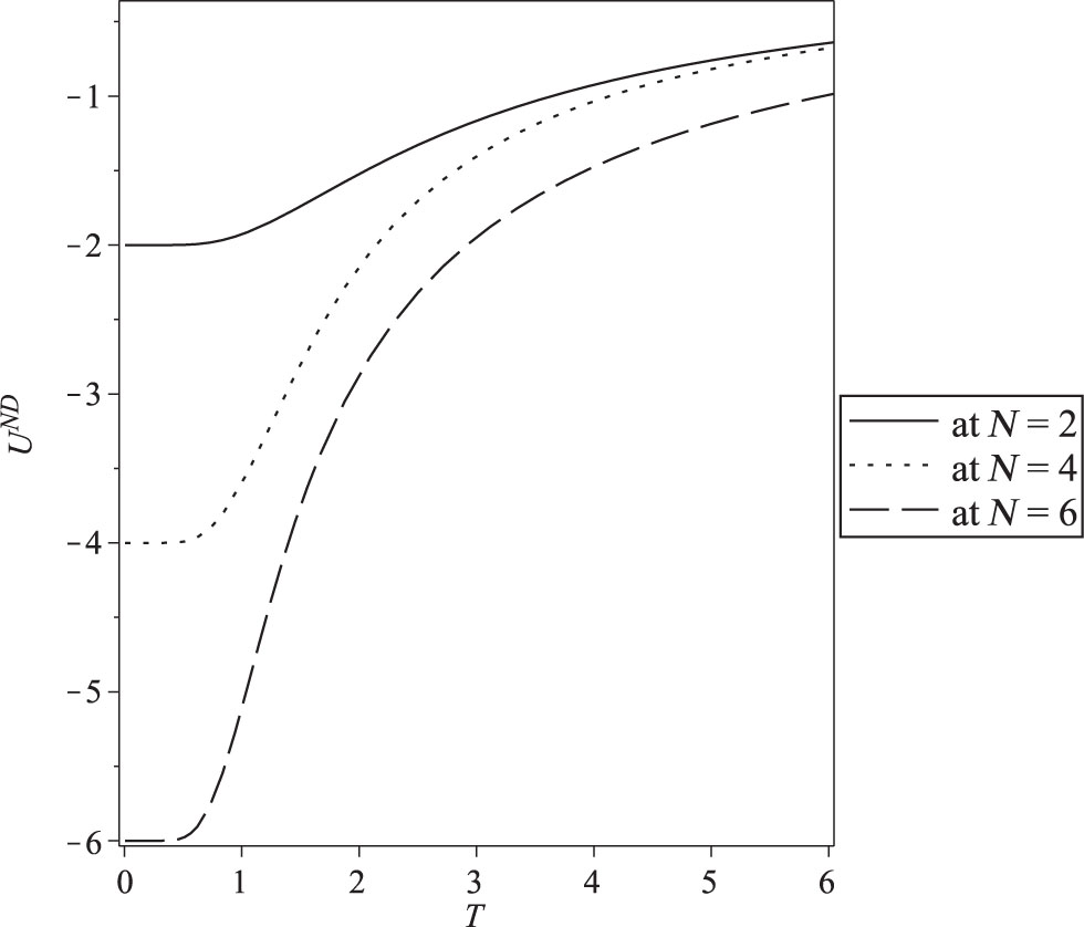
The internal energy as a function of temperature in the case of Neumann–Dirichlet boundary conditions for N = 2, 4, and 6.

Figure 2:

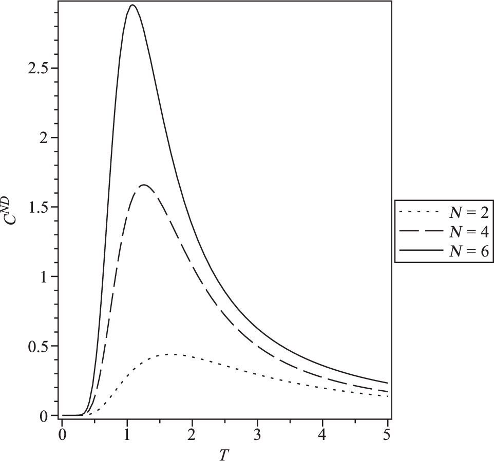
Heat capacity versus temperature when Neumann–Dirichlet boundary conditions are applied, for N = 2, 4, and 6.

Figure 3:

The entropy as a function of temperature in the case of Neumann–Dirichlet boundary conditions for N = 2, 4, and 6.

The exact results of the finite size properties of the one-dimensional Ising model versus temperature T (we take k_B = 1) for different values of the size N = 2, 4 and 6 in the case of Neumann–Dirichlet boundary conditions are presented in Figures 1–3. The dependence on the different boundary conditions is shown in Figures 4–6.

Results show that the internal energy is affected by increasing N and becomes constant and converges to zero at higher temperature values (Fig. 1). Figure 2 shows the temperature dependence of the heat capacity for different values of N. We notice that the heat capacity exhibits peak increases by increasing N. The entropy temperature dependence at different N is shown in Figure 3. At low temperature, the entropy becomes constant rapidly, and when T → 0, entropy goes to zero.

The use of the boundary conditions leads to a size dependence of the internal energy, the heat capacity, and the entropy (Figs. 4–6). We see that the properties belonging to the different boundary conditions are clearly distinct, thus demonstrating explicitly the boundary conditions dependence of the finite size properties of the model.

Figure 4:

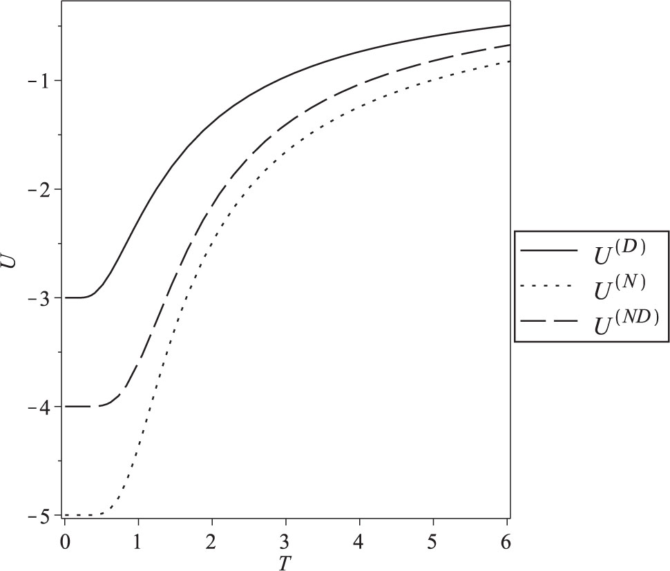
Internal energy in the presence of different boundary conditions for N = 4.

Figure 5:

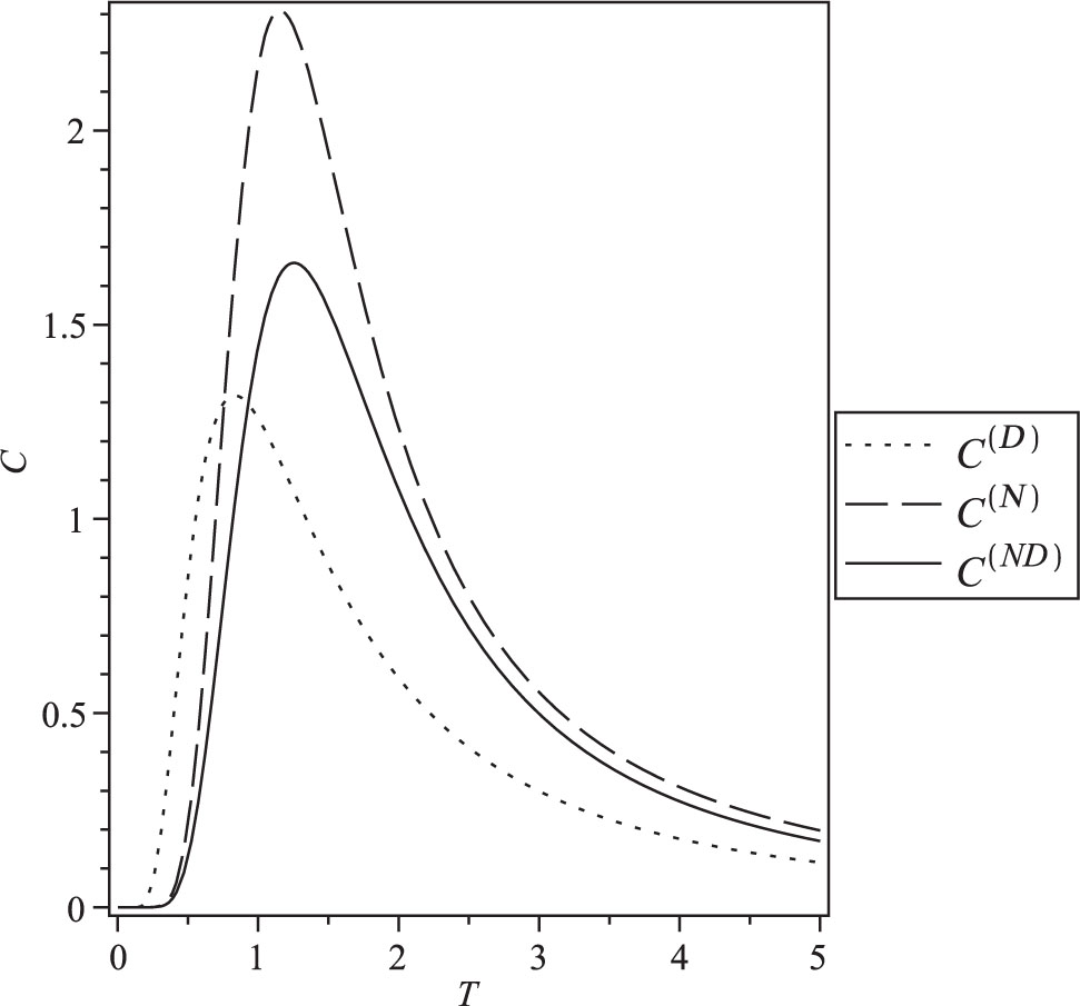
Heat capacity in the presence of different boundary conditions for N = 4.

Figure 6:

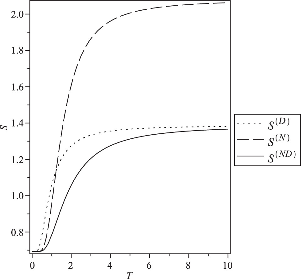
The entropy in the presence of different boundary conditions for N = 2.

4 Finite-Size Scaling Functions in the Presence of the External Field

In this section, our concentration will be in the one-dimensional Ising model with Neumann–Dirichlet boundary conditions in the presence of an external magnetic field. We now rewrite the partition function in the following form:

where K = βJ and H = βh are the reduced spin–spin nearest neighbour coupling energy and the reduced magnetic field. The partition function in this case can be calculated by using the transfer matrix method [12], [13]. The matrix elements T_{i, j} of the transfer matrix T may be written as follows:

The matrix elements of T can be computed directly from (17):

The partition function in (16) may now be written as follows:

where λ_i are the eigenvalues of T. They may be easily computed as T is 2 × 2. The characteristic equation is

which gives the two eigenvalues

In this case, the finite-size free energy is given by

In the thermodynamic limit N → ∞, the term (λ2/λ1)N will tend to zero as λ2/λ1<1. Hence, one obtains the bulk free energy:

Now all the properties of the model in the presence of the magnetic field can be obtained, but our focus will be devoted to studying the magnetic properties such as the magnetisation M(T, H) and the magnetic susceptibility χ (T, H). By direct calculations, the finite-size scaling functions of M(T, H) and χ (T, H) take the following form:

Figure 7:

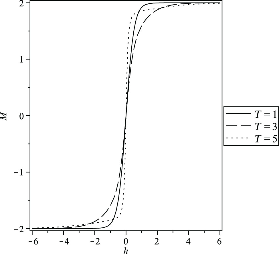
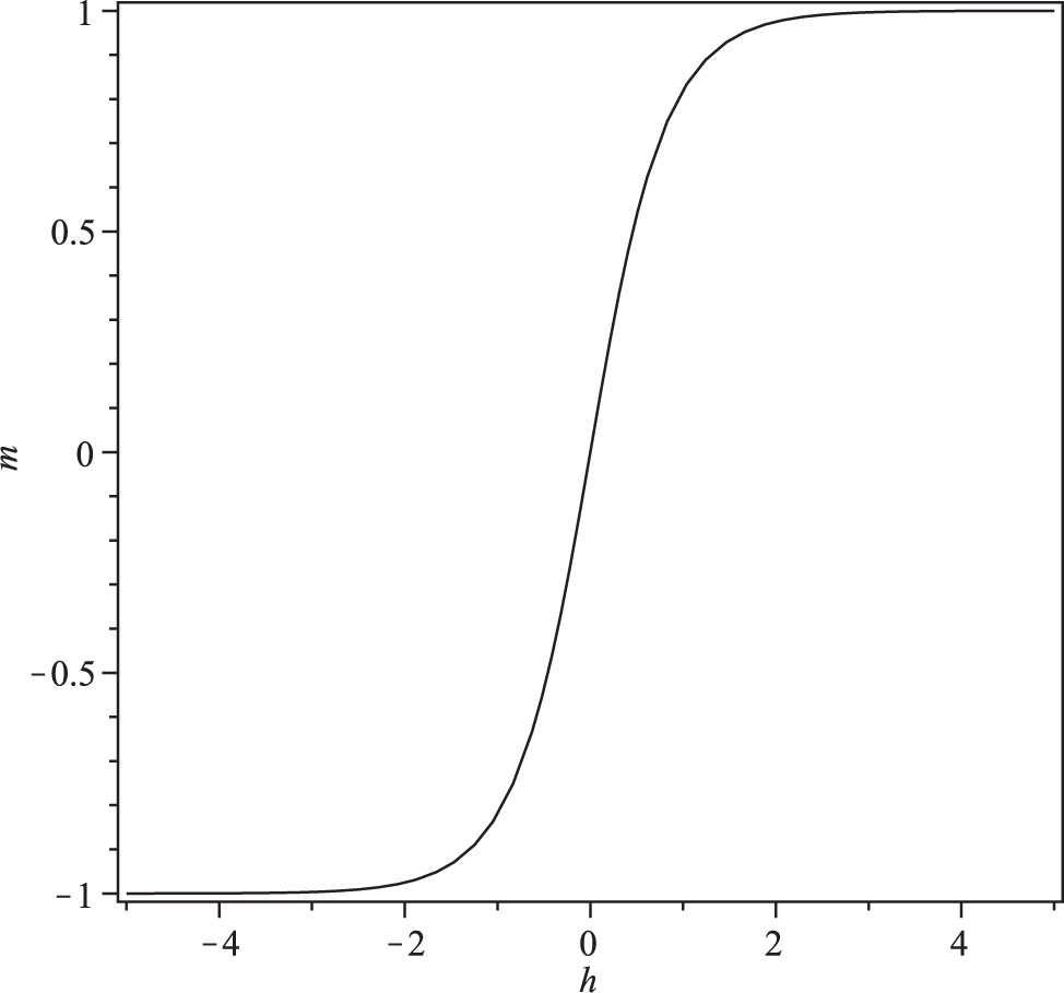
Magnetisation as a function of magnetic field at size N = 2 for different temperature T = 1, 3, and 5.

Figure 8:

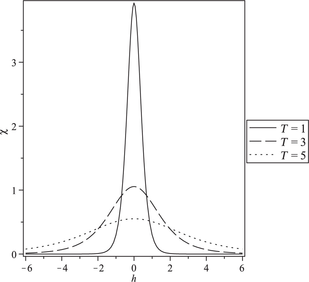
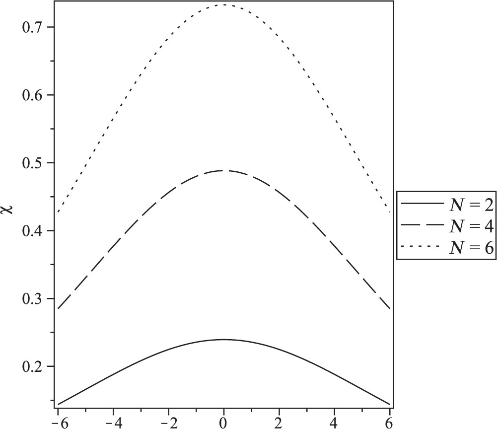
Magnetic susceptibility as a function of the field at size N = 2 for different values of temperature T = l, 3, and 5.

Figure 9:

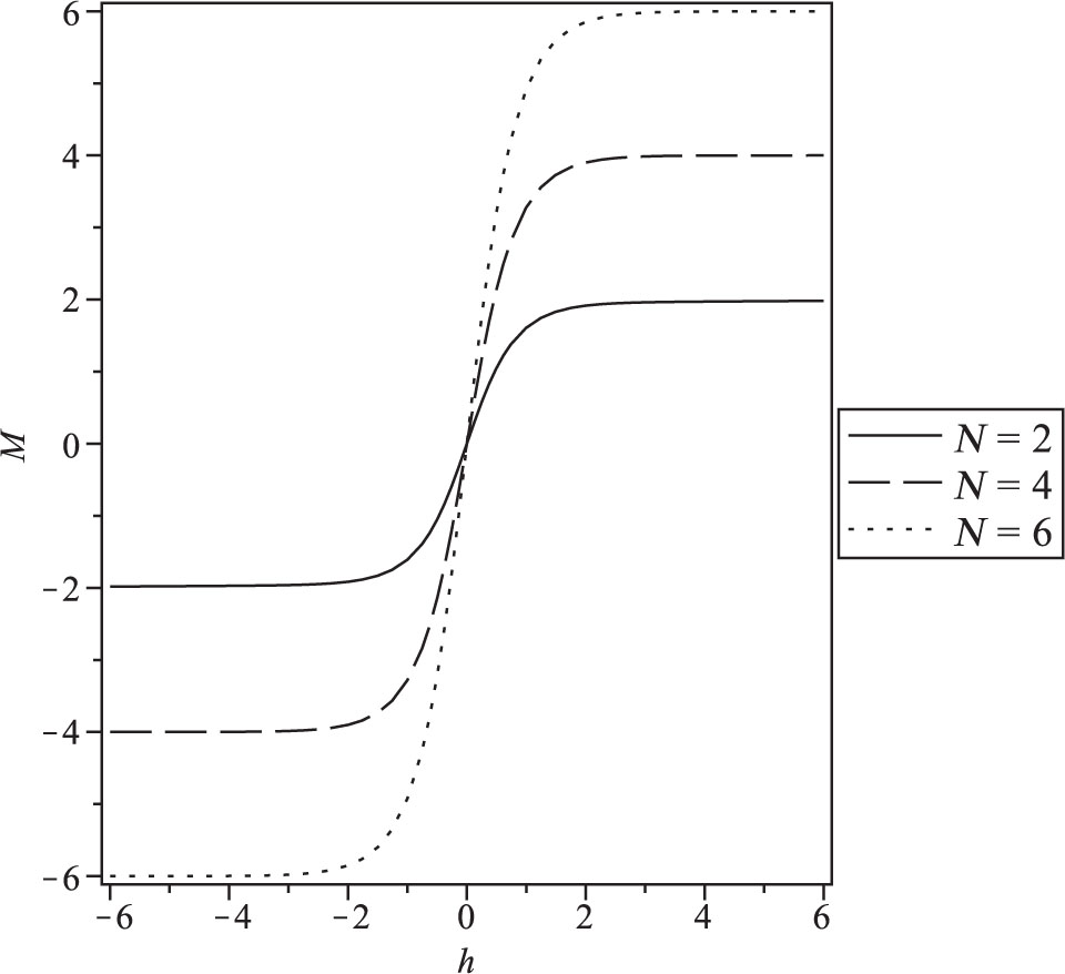
Magnetisation as a function of magnetic field at temperature T = 10 for different size N = 2, 4, and 6.

The behaviour of the magnetisation and the susceptibility as a function of the field under the effect of the temperature (T = 1, 3 and 5) are given in Figures 7 and 8 and in the presence of different sizes (N = 2, 4 and 6) are given in Figures 9 and 10.

We observe that the magnetisation behaviour with the change of the magnetic field is smoother with the increase in the temperature and becomes a step function in the limit of T → 0 corresponding to a ferromagnetic phase (Fig. 7).

The magnetic field dependence of the susceptibility is plotted in Figure 8 for different values of the temperature. The susceptibility peaks show that the maximum of χ (T, H) is larger for low temperature.

The effect of the size of the system on the magnetisation is observed in Figure 9. It is clear that increasing the size is accompanied by shifting the maximum value of the magnetisation. The same result was obtained for susceptibility (Fig. 10).

Figure 10:

Magnetic susceptibility as a function of magnetic field at temperature T = 10 for different size N = 2, 4, and 6.

Figure 11:

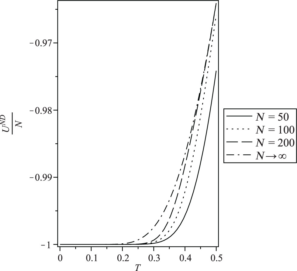
Internal energy per spin under Neumann–Dirichlet boundary conditions for N = 50, 100, and 200 compared with the bulk value N = ∞.

5 Bulk Properties of the Model

In the thermodynamic limit N → ∞, the finite-size scaling functions of the one-dimensional Ising model reduce to the bulk properties (intensive functions) in the well-known forms:

Figure 12:

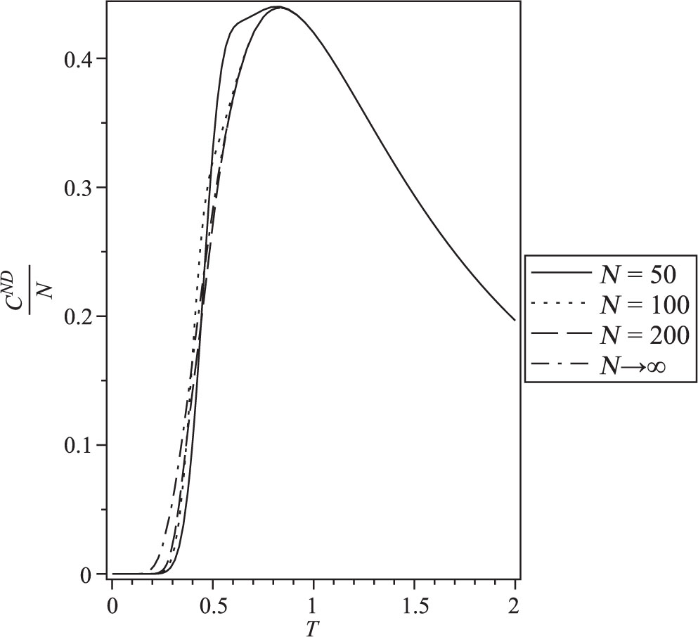
Heat capacity per spin under Neumann–Dirichlet boundary conditions for N = 50, 100, and 200 compared with the bulk value N = ∞.

Figure 13:

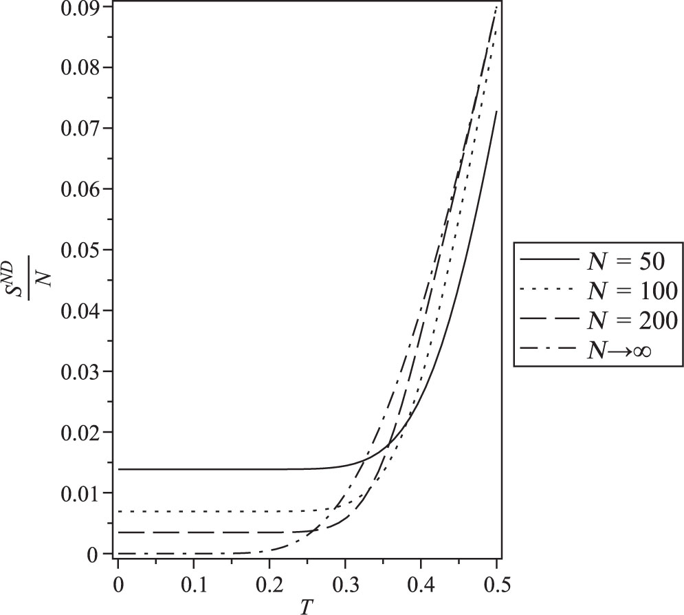
The entropy per spin under Neumann–Dirichlet boundary conditions for N = 50, 100, and 200 compared with the bulk value N = ∞.

The behaviour of the finite-size properties per spin in the case of Neumann–Dirichlet boundary conditions for N = 50, 100 and 200 compared with the bulk value N = ∞ (26) is plotted in Figures 11–14. Figure 11 indicates that the internal energy per spin increases with N, but the increases slow down for larger values of N where the curve for N = 200 approximates N = ∞ much better than N = 50. Again, the heat capacity per spin for N = 200 approaches the bulk value (Fig. 12). For the entropy per spin, the same behaviour is given in Figure 13; increasing size of the system will lead it to approach bulk value. In the presence of magnetic field, one has two eigenvalues; one of them is larger than the other. For small values of N, the two eigenvalues should be taken into account for computation of the magnetisation and the susceptibility (24 and 25), but for large values of N, the ratio λ2/λ1 is neglected. In Figure 14, we notice that the finite size of the magnetisation per spin for large N is in exact agreement with those of the infinite case.

Figure 14:

Magnetisation per spin under Neumann–Dirichlet boundary conditions for N = 50, 100, and 200 compared with the bulk value N = ∞.

6 Conclusions

The one-dimensional Ising model of finite sizes is considered. We investigated the effect of the finite size and the boundary conditions on the properties of the model. The thermodynamic properties such as internal energy, heat capacity, and entropy are derived exactly in the absence of magnetic field. It has been shown that the finite-size scaling of the thermodynamic properties is different from that of the infinite case and depends on the boundary conditions. The magnetic properties of the model are studied by using the transfer matrix method. We have performed the magnetisation and magnetic susceptibility as a function of the field under the effect of different temperatures and different sizes. We have shown that when the size of the system is limited the finite-size effect seems important as the deviation of the finite-size properties from the bulk values is large, and the deviation vanishes when N becomes large. Our results are consistent with the previous results on the one-dimensional Ising model.

References

[1] M. E. Fisher, in: Critical Phenomena, International School of Physics “Enrico Fermi” (Ed. M. S. Green), Academic Press, New York 1971, p. 1.Search in Google Scholar
[2] M. N. Barber, in: Phase Transition and Critical Phenomena (Eds. C. Domb, J. L. Lebowitz), Academic Press, London 1983, p. 144Search in Google Scholar
[3] V. Privman, in: Finite Size Scaling and Numerical Simulation of Statistical Systems (Ed. V. Privman), World Scientific, Singapore 1990, p. 1.10.1142/1011Search in Google Scholar
[4] J. G. Brankov, D. M. Danchev, and N. Tonchev, in: Theory of Critical Phenomena in Finite-Size Systems-Scaling and Quantum Effects, World Scientific, Singapore 2000, p. 1.10.1142/4146Search in Google Scholar
[5] K. Binder, Z. Phys. B 43, 119 (1981).10.1007/BF01293604Search in Google Scholar
[6] T. Anatal, M. Droz, G. Györgyi, and Z. Rácz, Phys. Rev. Lett. 87, 240601 (2001).10.1103/PhysRevLett.87.240601Search in Google Scholar PubMed
[7] T. Anatal, M. Droz, G. Györgyi, and Z. Rácz, Phys. Rev. E 65, 046140 (2002).10.1103/PhysRevE.65.046140Search in Google Scholar PubMed
[8] T. Anatal, M. Droz, and Z. Rácz, J. Phys. A 37, 1465 (2004).10.1088/0305-4470/37/5/001Search in Google Scholar
[9] E. Ising, Z. Phys. 31, 253 (1925).10.1007/BF02980577Search in Google Scholar
[10] K. Huang, Statistical Mechanics, John Wiley and Sons Inc., New York 1987.Search in Google Scholar
[11] R. K. Pathria, Statistical Mechanics, Elsevier, Amsterdam 1996.Search in Google Scholar
[12] H. A. Kramers and G. H. Wannier, Phys. Rev. 60, 252 (1941).10.1103/PhysRev.60.252Search in Google Scholar
[13] R. K. Pathria and P. D. Beale, Statistical Mechanics, Academic Press, Elsevier 2011.Search in Google Scholar
©2020 Walter de Gruyter GmbH, Berlin/Boston
Articles in the same Issue
- Frontmatter
- Atomic, Molecular & Chemical Physics
- Numerical Investigation of the Cooling Temperature of the InGaP/InGaAs/Ge Subcells Under the Concentrated Illumination
- Dynamical Systems & Nonlinear Phenomena
- Ion-Acoustic Cnoidal Waves with the Density Effect of Spin-up and Spin-down Degenerate Electrons in a Dense Astrophysical Plasma
- Hydrodynamics
- Landau Quantised Modification of Rayleigh–Taylor Instability in Dense Plasmas
- Interaction of a Singular Surface with a Characteristic Shock in a Relaxing Gas with Dust Particles
- Quantum Theory
- Path Integrals, Spontaneous Localisation, and the Classical Limit
- Proposal for a New Quantum Theory of Gravity III: Equations for Quantum Gravity, and the Origin of Spontaneous Localisation
- Quantum-Phase-Field: From de Broglie–Bohm Double-Solution Program to Doublon Networks
- Solid State Physics & Materials Science
- Photovoltaic Generator Based on Laser-Induced Reversible Aggregation of Magnetic Nanoparticles
- Thermodynamics & Statistical Physics