Rogue Waves and New Multi-wave Solutions of the (2+1)-Dimensional Ito Equation

1 Introduction

It is well known that high-dimensional nonlinear wave systems have richer behaviour than one-dimensional ones. It has been shown that different structures of solitons peculiar to higher dimensionality may contribute to a variety of dynamics of nonlinear waves [1–5]. Therefore, the investigation of various structures of exact solutions is imperative for physics and mathematics to the complexity and variety of dynamics determined by high-dimensional nonlinear evolution equations (NEEs) [6–10].

Recently, the rogue wave phenomenon was popular in nonlinear science. Rogue waves are large and spontaneous nonlinear waves and have drawn much attention in some fields of nonlinear science such as oceanics [11–13], nonlinear optics [14–16], Bose–Einstein condensations [17], and even finance [18, 19]. It has been found that several nonlinear equations possessing rogue waves and rational solutions, such as the nonlinear Schrödinger equation (NLSE) [20, 21], the derivative NLSE [22, 23], the generalised NLSE [24, 25], the Hirota equation [26], the Kadomtsev–Petviashvili (KP) equation [27], the Davey–Stewartson equations [28, 29], the Boussinesq equation [30, 31], the couped NLSE [32], the higher-order Hirota system [33], and the Toda lattice equation [34]. In order to find rogue wave and rational solutions of nonlinear wave systems, some effective methods have been proposed, such as the D. H. Peregrine method, homoclinic test approach, the Akhmdiev breather method, extended homoclinic test approach, homoclinic test limit method, the Wronskian technique, and so on [11–37]. In this work, we propose a three-soliton limit method (TSLM) to seek rogue waves to NEE. Let us consider a general nonlinear partial differential equation in the form

P(u, ut, ux, uy, uxx, uxy, uxt…) = 0,

where P is a polynomial in its arguments, and u : R_x×R_y×R_t → R. To determine the function u(x, y, t) explicitly, we take the following three steps:

Step 1. By the Painlevé analysis, a transformation

u = T(f)

is made for some new and unknown function f. By using this transformation, the original equation can be transformed into Hirota’s bilinear form

G(Dx, Dy, Dt; f) = 0,

where the Hirota bilinear operator D, e.g., for two-variable functions, is defined as

DxmDtnf(x, t) ⋅ g(x, t) = (∂∂x−∂∂x′)m(∂∂t−∂∂t′)n[f(x, t)g(x′, t′)]|x′ = x, t′ = t.

Step 2. Solve the preceding equation to get some multi-wave solutions to the original equation by using modified three-soliton method [38].

Step 3. In order to get rational solutions (rogue waves), let some parameter tend to be zero in some multi-wave solutions obtained in Step 2.

As an example, let us consider the well-known (2+1)-dimensional Ito equation established by Ito in 1980 [39]. The (2+1)-dimensional Ito equation reads as

(1)utt + uxxxt + 32uxut + uuxt) + 3uxx∫−∞xutdx′ + auyt + buxt = 0, (1)

where a, b are constants; u= u(x, y, t) is an unknown function of independent variables x, y, t; and the subscripts denote partial derivatives. The (2+1)-dimensional Ito equation (1) is reduced to (1+1) dimensional when a= 0, b= 0 [39].

There have been some studies concerning the (2+1)-dimensional Ito equation (1) [39–45]. But to the best of out knowledge, rogue waves to the Ito equation (1) have not been reported in previous literatures. This work focusses on new multi-wave solutions and then rogue wave solutions of (1). Applying TSLM to (1), we first get some new multi-wave solutions and then obtain two rational solutions by letting some parameter tend to be zero in breather solitary wave solution and double-breather solitary wave solution. Finally, we show that the rational solutions are just rogue waves. It is a new and interesting discovery that rogue wave can be obtained from extreme behavior of double-breather solitary wave.

2 Multi-wave Solutions

By applying the truncated Painlevé expansion, we assume

(2)u = 2(ln f)xx, (2)

where f= f(x, y, t) is an unknown function. Substituting transformation (2) into (1), the bilinear equation of (1) is found to be

(3)Dt(Dt + Dx3 + aDy + bDx)f ⋅ f = 0, (3)

Using modified three-soliton method, we choose the function

(4)f = e−ξ + Acosη + Bcoshτ + Ceξ, (4)

where ξ= p(x + a₁y + b₁t), η= q(x + a₂y + b₂t), τ= r(x + a₃y + b₃t) and A, B, C, p, q, r, a_i, b_i(i= 1, 2, 3) are some constants to be determined later.

Substituting (4) into (3) and equating all the coefficients of e^ξ, e^–ξ, sinη, cosη, sinhτ, coshτ and constant term to zero, we can obtain a set of nonlinear algebraic equations for A, B, C, p, q, r, a_i, b_i (i= 1, 2, 3). Solving the system with the aid of Maple, we get the following results.

Case 1:

(5)B = 0, a1 = − bq2A2 + aA2q2a2 + 4p2Cb − A2q4 + 3q2A2p2 − 12p2Cq2 + 4p4C4aCp2,b1 = q2A2(b + aa2 + 3p2 − q2)4Cp2, b2 = − b − aa2 − 3p2 + q2, (5)

where A, C, p, q, a₂ are free real constants.

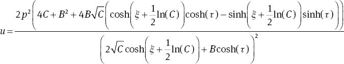
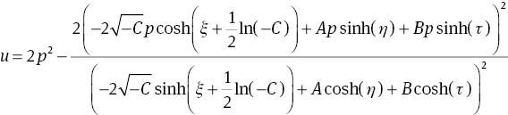
Substituting (4) into (2) with (5), we obtain the following breather solitary waves of (1):

(6)u = 2(4Cp2 − A2q2 + 2AC(p2 − q2)cosh(ξ + 12ln(C))cos(η) + 4ACpqsinh(ξ + 12ln(C))sin(η))(2Ccosh(ξ + 12ln(C)) + Acos(η))2 (6)

for C>0, and

(7)u = 2(4Cp2 − A2q2 − 2A−C(p2 − q2)sinh(ξ + 12ln(−C))cos(η) − 4A−Cpqcosh(ξ + 12ln(−C))sin(η))(−2−Csinh(ξ + 12ln(−C)) + Acos(η))2 (7)

for C<0, where ξ = p(x − bq2A2 + aA2q2a2 + 4p2Cb − A2q4 + 3q2A2p2 − 12p2Cq2 + 4p4C4aCp2y + q2A2(b + aa2 + 3p2 − q2)4Cp2t), η = q(x + a2y − (b + aa2 + 3p2 − q2)t).

Case 2:

(8)A = 0, B = B, C = C, a1 = −4p2 + b1 + ba, b3 = −4p2 − aa3 − b, r = p, (8)

where B, C, p, b₁, a₃ are free real constants.

Substituting (4) into (2) with (8), we find the following two-soliton solutions of (1):

(9)u = 2p2(4C + B2 + 4BC(cosh(ξ + 12ln(C))cosh(τ) − sinh(ξ + 12ln(C))sinh(τ)))(2Ccosh(ξ + 12ln(C)) + Bcosh(τ))2 (9)

for C>0, and

(10)u = 2p2(4C + B2 + 4B−C(cosh(ξ + 12ln(−C))sinh(τ)−sinh(ξ+12ln(−C))cosh(τ)))(−2−Csinh(ξ + 12ln(−C)) + Bcosh(τ))2 (10)

for C<0, where ξ = p(x − 4p2 + b1 + bay + b1t), τ = p(x + a3y − (4p2 + aa3 + b)t).

Case 3:

(11)C = B2p2b1 − A2q2b24b1p2, a1 = −b1 + b + p2 − 3q2a, a2 = −b2 + b + 3p2 − q2a, a3 = −−b1 + b + p2 − 3q2a, b3 = −b1, r = p, (11)

where A, B, p, q, b₁, b₂ are free real constants.

It is easy to see that C>0 if and only if (b₂/b₁)<(B²p² / A²q²). Substituting (4) into (2) with (11), we get the following breather double-soliton solutions to (1):

(12)u = 2(2Cp2cosh(ξ + 12ln(C)) − Aq2cos(η) + Bp2cosh(τ))2Ccosh(ξ + 12ln(C)) + Acos(η) + Bcosh(τ) − 2(2Cpsinh(ξ + 12ln(C)) − Aqsin(η) + Bpsinh(τ))2(2Ccosh(ξ + 12ln(C)) + Acos(η) + Bcosh(τ))2 (12)

for (b₂/b₁)<(B²p² / A²q²), and

(13)u = 2(−2−Cp2sinh(ξ + 12ln(−C)) − Aq2cos(η) + Bp2cosh(τ))−2−Csinh(ξ + 12ln(−C)) + Acos(η) + Bcosh(τ) − 2(−2−Cpcosh(ξ + 12ln(−C)) − Aqsin(η) + Bpsinh(τ))2(−2−Csinh(ξ + 12ln(−C)) + Acos(η) + Bcosh(τ))2 (13)

for (b₂/b₁)>(B²p² / A²q²), where ξ = p(x − b1 + b + p2 − 3q2ay + b1t), η = q(x − b2 + b + 3p2 − q2ay + b2t), τ = p(x − −b1 + b + p2 − 3q2ay − b1t).

Case 4:

(14)r = −iq, B = A, C = C, a1 = −p2 + b − 3q2a, b1 = 0, a2 = −3p2 − q2 + b + b2a, a3 = −3p2 − q2 + b − b2a, b3 = −b2, (14)

where A, C, p, q, b₂ are free real constants.

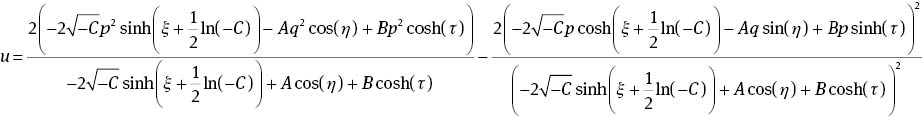
Substituting (4) into (2) with (14), one can get the following double-breather solitary waves of (1):

(15)u = 2(2Cp2cosh(ξ + 12ln(C)) − Aq2cos(η) − Aq2cos(τ))2Ccosh(ξ + 12ln(C)) + Acos(η) + Acos(τ) − 2(2Cpsinh(ξ + 12ln(C)) − Aqsin(η) − Aqsin(τ))2(2Ccosh(ξ + 12ln(C)) + Acos(η) + Acos(τ))2 (15)

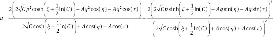
for C>0, and

(16)u = 2(−2−Cp2sinh(ξ + 12ln(−C)) − Aq2cos(η) − Aq2cos(τ))−2−Csinh(ξ + 12ln(−C)) + Acos(η) + Acos(τ) − 2(−2−Cpcosh(ξ + 12ln(−C)) − Aqsin(η) − Aqsin(τ))2(−2−Csinh(ξ + 12ln(−C)) + Acos(η) + Acos(τ))2 (16)

for C<0, where ξ = p(x − p2 − 3q2 + bay), η = q(x − 3p2 − q2 + b + b2ay + b2t), τ = q(x − 3p2 − q2 + b − b2ay − b2t).

Case 5:

(17)q = ip, r = p, A = A, B = B, C = C, b1 = −4p2 − b − aa1, b2 = −4p2 − b − aa2, a3 = −4p2 + ba, b3 = 0, (17)

where A, B, C, p, a₁, a₂ are free real constants.

Substituting (4) into (2) with (17), we obtain three-soliton solutions of (1) as follows:

(18)u = 2p2 − 2(2Cpsinh(ξ + 12ln(C)) + Apsinh(η) + Bpsinh(τ))2(2Ccosh(ξ + 12ln(C)) + Acosh(η) + Bcosh(τ))2 (18)

for C>0, and

(19)u = 2p2 − 2(−2−Cpcosh(ξ + 12ln(−C)) + Apsinh(η) + Bpsinh(τ))2(−2−Csinh(ξ + 12ln(−C)) + Acosh(η) + Bcosh(τ))2 (19)

for C<0, where ξ = p(x + a1y − (4p2 + b + aa1)t), η = p(x + a2y − (4p2 + b + aa2)t), τ = p(x − 4p2 + bay).

The earlier solutions have not been reported in previous literatures. They are new multi-wave solutions of the (2+1)-dimensional Ito equation (1).

3 Rogue Waves and Rational Solutions

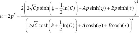
In order to obtain rational solution of the (2+1)-dimensional Ito equation (1), we consider the extreme behaviour of the breather solitary wave (6) (see Fig. 1a) and the double-breather solitary wave (15) (see Fig. 1b). If taking A= –2cos(p), C= 1, p= q in the breather solitary wave (6) and then letting p → 0, one can find a rational solution of (1):

Figure 1:

(a) The figure of the breather solitary wave (6) with A= –1, C= 1, p=q=1/2, a₂=1, a=b=1, t=0. (b) The figure of the double-breather solitary wave (15) with A=–(1/2), C=1, p=q=1, b₂=1, a=b=1, t=0.

(20)u = 8 + 8(x − 2b + aa2ay + (b + aa2)t)2 + 8(x + a2y − (b + aa2)t)2 − 32(x − bay)2(1 + (x − 2b + aa2ay + (b + aa2)t)2 + (x + a2y − (b + aa2)t)2)2, (20)

where a₂ is a free real constant. The rational solution (20) is nonsingular and is just a rogue wave (see Fig. 2a), From Figure 2a, we can see that the rogue wave takes maximal value 8 at (0,0) and has two to three times amplitude than its surrounding waves.

Figure 2:

(a) The figure of the rogue wave (20) with a₂=1, a=b=1, t=0. (b) The figure of the rogue wave (21) with b₂=2, a=b=1, t=1.

If we choose A = −cos(p), C = 1, q = 2p in the double-breather solitary wave (15) and then let p → 0, we can obtain the following rational solution of (1):

(21)u = 12 + 12(x − b + b2ay + b2t)2 + 12(x − b − b2ay − b2t)2 − 60(x − bay)2(1 + (x − b + b2ay + b2t)2 + (x − b − b2ay − b2t)2 + (x − bay)2)2, (21)

where b₂ is a free real constant. The solution (21) is also a rogue wave (see Fig. 2b). From Figure 2b, we can find that the rogue wave has maximal value 12 at (1,1). It is easy to see that the rogue waves (20) and (21) are different from each other. To the best of our knowledge, it is a new and interesting discovery that rogue wave can be obtained from the extreme behaviour of double-breather solitary wave.

4 Conclusion

In this work, we propose a TSLM for finding rogue waves of NEE. Applying the method to the (2+1)-dimensional Ito equation, we obtain a family of new multi-wave solutions and two rational solutions. Furthermore, the rational solutions obtained here are just rogue waves. We find that rogue wave can be obtained not only from the extreme form of breather solitary wave, but also from the extreme form of double-breather solitary wave. This is a new and interesting discovery. Our results show the complexity and variety of dynamical behaviour of the (2+1)-dimensional Ito equation. The method in this work can be used to discuss other NEE (especially in higher dimension).

References

[1] M. Tajiri and T. Arai, in: Proceedings of the Institute of Math. of NAS of Ukraine 30, 210 (2000).Search in Google Scholar
[2] E. Yomba, Chaos Solitons Fract. 22, 321 (2004).10.1016/j.chaos.2004.02.001Search in Google Scholar
[3] M. J. Ablowitz and P. A. Clarkson, Solitons, Nonlinear Evolution Equation and Inverse Scattering, Cambrige Universicity Press, Cambrige 1991.10.1017/CBO9780511623998Search in Google Scholar
[4] B. Konopechenko, Solitons in Mathematics, Inverse Spectral Transform Method, Word Scientific Press, Singapore 1993.Search in Google Scholar
[5] Z. D. Dai, S. L. Li, and D. L. Li, Chin. Phys. Lett. 24, 1429 (2007).Search in Google Scholar
[6] S. J. Yu, K. Tota, and N. Sasa, J. Phys. A Math. Gen. 31, 3337 (1998).10.1088/0305-4470/31/14/018Search in Google Scholar
[7] J. Schff, Painlevé Transendent, Their Asymptotics and Physical Applications, Plenum, New York 1992.Search in Google Scholar
[8] W. X. Ma and Z. Zhu, Appl. Math. Comput. 218, 11871 (2012).10.1016/j.amc.2012.05.049Search in Google Scholar
[9] Y. J. Hu, H. L. Chen, and Z. D. Dai, Appl. Math. Comput. 234, 548 (2014).10.1016/j.amc.2014.02.044Search in Google Scholar
[10] W. Chen, H. L. Chen, and Z. D. Dai, Commun. Ther. Phys. 62, 707 (2014).10.1088/0253-6102/62/5/13Search in Google Scholar
[11] P. Muller, C. Garrett, and A. Osborne, Oceanography 18, 65 (2005).10.5670/oceanog.2005.30Search in Google Scholar
[12] D. H. Peregrine, J. Austral. Math. Soc. Ser. B. 25, 16 (1983).10.1017/S0334270000003891Search in Google Scholar
[13] C. Kharif, E. Pelinovsky, and A. Sunyaey, Rogue Waves in the Ocean, Observation, Theories and Modeling, Spinger, New York 2009.Search in Google Scholar
[14] N. Akhmediev, A. Ankiewicz, and J. M. Soto-Crespo, Phys. Rev. E 80, 026601 (2009).10.1103/PhysRevA.80.043818Search in Google Scholar
[15] D. R. Solli, C. Ropers, P. Koonath, and B. Jalali, Nature 450, 1054 (2007).10.1038/nature06402Search in Google Scholar PubMed
[16] V. Yu. Biudov, V. V. Konotop, and N. Akhmediev, Opt. Lett. 34, 3015 (2009).10.1364/OL.34.003015Search in Google Scholar
[17] V. Yu. Bludov, V. V. Konotop, and N. Akhmediev, Phys. Rev. A. 80, 033610 (2009).10.1103/PhysRevA.80.033610Search in Google Scholar
[18] Z. Y. Yan, Phys. Lett. A. 375, 4274 (2011).10.1016/j.physleta.2011.09.026Search in Google Scholar
[19] Z. Y. Yan, Commun. Ther. Phys. 54, 947 (2010).10.1088/0253-6102/54/5/31Search in Google Scholar
[20] N. Akhmediev, A. Ankiewicz, and M. Taki, Phys. Lett. A. 373, 675 (2009).10.1016/j.physleta.2008.12.036Search in Google Scholar
[21] A. Ankiewcz, D. J. Kedziora, and N. Akhmediev, Phys. Lett. A. 375, 2782 (2011).10.1016/j.physleta.2011.05.047Search in Google Scholar
[22] S. W. Xu, J. S. He, and L. H. Wang, J. Phys. A Math. Theor. 44, 305203 (2011).10.1088/1751-8113/44/30/305203Search in Google Scholar
[23] S. W. Xu and J. S. He, J. Math. Phys. 53, 063507 (2012).10.1063/1.4726510Search in Google Scholar
[24] L. H. Wang, K. Porsezian, and J. S. He, Phys. Rev. E. 87, 053202 (2013).10.1103/PhysRevE.87.069904Search in Google Scholar
[25] Zhaqilao, Phys. Lett. A. 377, 855 (2013).10.1016/j.physleta.2013.01.044Search in Google Scholar
[26] G. Y. Yang, L. Li, and S. T. Jia, Phys. Rev. E. 85, 046608 (2012).10.1103/PhysRevE.85.046608Search in Google Scholar
[27] Y. F. Guo, L. M. Ling, and Z. D. Dai, Commun. Ther. Phys. 59, 723 (2013).10.1088/0253-6102/59/6/13Search in Google Scholar
[28] Y. Ohta and J. K. Yang, Phys. Rev. E. 86, 036604 (2012).10.1103/PhysRevE.86.036604Search in Google Scholar
[29] Y. Ohta and J. K. Yang, J. Phys. A Math. Theor. 46, 105202 (2013).10.1088/1751-8113/46/10/105202Search in Google Scholar
[30] W. X. Ma, C. X. Li, and J. S. He, Nonlinear Anal. 70, 4245 (2009).10.1016/j.na.2008.09.010Search in Google Scholar
[31] P. A. Clakson, Anal. Appl. 6, 349 (2008).10.1142/S0219530508001250Search in Google Scholar
[32] L. X. Li, J. Liu, Z. D. Dai, and R. L. Liu, Z. Naturforsch. 69a, 441 (2014).Search in Google Scholar
[33] D. W. Zuo, Y. T. Gao, Y. H. Sun, Y. J. Feng, and L. Xue, Z. Naturforsch. 69a, 521 (2014).10.5560/zna.2014-0045Search in Google Scholar
[34] W. X. Ma and Y. You, Chaos Solitons Fractals. 22, 395 (2004).10.1016/j.chaos.2004.02.011Search in Google Scholar
[35] N. Akhmediev, J. M. Soto-Crespo, and A. Ankiewicz, Phys. Lett. A. 373, 2137 (2009).10.1016/j.physleta.2009.04.023Search in Google Scholar
[36] Z. H. Xu, H. L. Chen, and Z. D. Dai, Appl. Math. Lett. 37, 34 (2014).10.1016/j.aml.2014.05.005Search in Google Scholar
[37] H. L. Chen, Z. H. Xu, and Z. D. Dai, Abstr. Appl. Anal. 2014, (2014) Article ID 378167.Search in Google Scholar
[38] Z. D. Dai and C. J. Wang, Nonlinear Sci. Lett. A. 1, 77 (2010).Search in Google Scholar
[39] M. Ito, J. Phys. Soc. Jpn. 49, 771 (1980).10.1143/JPSJ.49.771Search in Google Scholar
[40] A. Ceaser and S. Gomez, Appl. Math. Comput. 216, 241 (2010).Search in Google Scholar
[41] Z. H. Zhao, Z. D. Dai, and C. J. Wang, Appl. Math. Comput. 217, 2295 (2010).10.1016/j.amc.2010.06.059Search in Google Scholar
[42] D. Li and J. Zhao, Appl. Math. Comput. 215, 1968 (2009).10.1016/j.amc.2009.07.058Search in Google Scholar
[43] Q. Liu, Phys. Lett. A. 227, 31 (2000).10.1353/nlh.2000.0014Search in Google Scholar
[44] A. M. Wazwaz, Appl. Math. Comput. 202, 840 (2008).10.1016/j.amc.2008.03.029Search in Google Scholar
[45] G. Ebadi, A. H. Kara, M. D. Petkovic, A. Yildirim, and A. Biswas, Proc. Rom. Acad. Ser. A. 13, 215 (2012).Search in Google Scholar
©2015 by De Gruyter
Articles in the same Issue
- Frontmatter
- A Note on Exact Solutions for the Unsteady Free Convection Flow of a Jeffrey Fluid
- Equation of State, Nonlinear Elastic Response, and Anharmonic Properties of Diamond-Cubic Silicon and Germanium: First-Principles Investigation
- Quantum Electron-Exchange Effects on the Buneman Instability in Quantum Plasmas
- Diffraction of Pulsed Sound Signals by Elastic Bodies of Analytical and Non-analytical Forms, Put in Plane Waveguide
- Density Functional Theory Calculations of H/D Isotope Effects on Polymer Electrolyte Membrane Fuel Cell Operations