Spectral reconstruction using neural networks in filter-array-based chip-size spectrometers

1.1 Related works

In spectral reconstruction, two main principles have become apparent in the literature. First, one could reconstruct spectral data from RGB images by extrapolating additional information from the three color channels. The main goal of this approach is to circumvent the need for expensive hyper-spectral cameras while simultaneously acquiring spatial and spectral information. In [10], Zhang et al. highlight the most relevant approaches to spectral reconstruction on RGB images. Secondly, instead of relying on just three color channels, filter-array-based sensors can capture more spectral information, albeit at the expense of spatial resolution. These sensors usually replace classic spectrometers, which feature a high spectral resolution for point measurements. As we base this work on a filter-array spectral sensor, the following discussion of related work will focus on spectral reconstruction methods specific to this type of sensor.

Previous publications have added techniques that are considered state-of-the-art to stabilize the reconstruction. [11] uses adaptive Tikhonov regularization to stabilize the reconstruction result successfully. In [12], the authors use singular value decomposition with regularization to find solutions more quickly while maintaining accuracy. However, these methods were designed for miniature spectrometers, which are still large and expensive compared to a chip-size-spectrometer (CSS). To further decrease sensor cost and size, filters utilized in chip-scale spectrometers may exhibit inferior filter characteristics, with the sensitivity of each filter not confined to a narrow wavelength range. Additionally, cross-talk between filters and noise is becoming more problematic with a smaller sensor footprint. Therefore, recent publications aid their reconstructions with NNs for an improved result. In [8], the authors apply an Auto-Encoder to denoise the raw sensor data before the reconstruction process. Furthermore, the same authors employ a Multi-Layer-Perceptron (MLP) after reconstruction, i.e., at the other end of the processing pipeline, to correct its output [7].

2.1 Sensor setup

A key aspect of training an effective machine-learning model for spectral reconstruction is having a data set that is rich enough to cover as many different non-trivial spectra as possible while still having enough redundancy to depict deviations from manufacturing and sensor noise. As this work uses an internally developed CSS with a novel filter structure, no publicly available data set can fulfill the points mentioned above. Therefore, we have to collect our own data set.

The working principles of various filter-based miniature spectrometers are usually quite similar. Filter structures are applied on top of photodiodes, which filter out certain wavelengths, rendering each photodiode sensitive only to specific sections of the light spectrum. Arranged in an array, these diodes form a two-dimensional spectral sensor. The distinction among sensor technologies is in the manufacturing of the filters themselves. One such manufacturing technique is Colloidal Quantum Dots [7], [8], which the authors from the MLP-aided reconstructions use in their publications mentioned in Section 1.1. In contrast, the spectrometer used in this work functions with plasmonic color filters that make use of different-sized holes introduced into the metal layers of the CMOS process [13], [14], [15]. Further filtering techniques [16] are also possible but out of the scope of this work. The CSS used here consists of an array of 40 × 40 diodes, therefore totaling 1,600 spectral filters. The array is divided further into so-called meta-pixels with 4 × 4 filters, as shown in Figure 1. This division results from the manufacturing and sensor design, making one 4 × 4 array of filters placable and readable by the readout circuitry as a block. The filters inside each meta-pixel are designed by a controlled variation of the holes. This causes an ascending order in target wavelengths, leading to a marginal spatial relationship inside a meta-pixel. The placing of the meta-pixels on the chip does not follow any specifications. However, some further relations still exist. Different manufacturing techniques were tested to build the meta-pixels as the chip was developed in a research project. Therefore, some pixels might still react similarly to incoming light. As ground truth measurements, we utilize Broadcom’s QMini Wide VIS spectrometer, which can measure the spectrum from 225 nm to 1,000 nm. The colored foils are transparent to wavelengths above 700 nm. Therefore, we use an IR filter to block out the light above 700 nm and limit the considered wavelength range to 690 nm to prevent the edge effects of said filter. Additionally, the filters on the CSS are not sensitive to wavelengths below 450 nm. This results in a 1 × 240 output dimensionality to achieve 1 nm resolution in the reconstructed spectrum. As a last pre-processing step, we normalize both the CSS measurements and the ground truth data. The normalized spectrum of one filter channel

can be obtained by subtracting a dark measurement r n d without a light source from the raw measurement r _n and dividing the result by a white measurement with just the light source r n w , also corrected by the dark measurement. As all filter foils used for the dataset have a transmittance between 0 and 1, dividing by a white measurement equals dividing by the maximum possible value for each respective channel and wavelength. The subtraction of dark counts ensures that the input values are also around 0 in the absence of light, correcting for any remaining dark current.

Figure 1:

CSS-measurement with 40 × 40 filters. The meta-pixel grouping is indicated as a black grid.

2.2 Neural network architectures for reconstruction

We test various NN architectures ranging from simple dense over convolutional to transformer-based networks. The simplest NN is the dense network, which comprises five hidden layers with [2,560, 1,024, 512, 256, 256] neurons and ReLU activations (cf. Figure 2). We highlight the other networks in the following subsections.

Figure 2:

Network architecture of the CNN and dense model. For the CNN architecture, the output of the convolutional layers is forwarded into the input of the dense network.

2.2.2 Transformer-based networks

Recently, a new type of architecture has gained popularity as a tool for visual recognition tasks. Vision Transformers have improved performance compared to CNNs in many image processing problems. To understand their differences from CNNs and why they could probably also perform better for the problem of spectral reconstruction, we want to highlight the underlying architecture briefly.

Google introduced the transformer in 2017 based on the attention mechanism for natural language processing (NLP) [20]. Before, the encoder-decoder architecture or recursive NNs, which process each sentence in the written order, dominated the field of NLP [20]. However, it is possible that consecutive words do not necessarily depend on each other but rather on different aspects of a sentence. To solve this problem, the authors applied the attention layers as an extension to the encoder-decoder. In this way, the network can assign weights to different parts of the input sentence depending on their importance. Following its success, Google quickly adapted the transformer for image processing tasks. This Vision Transformer (ViT) [21] can similarly process an image by splitting the input in different patches and finding relations in between them (cf. Figure 3a). We apply the ViT as the first transformer-based architecture to test for spectral reconstruction. The dimensions specified in Figure 3a already describe the dimensions used to adapt the input to our frame size. By setting the patch size equal to the meta-pixel size, we expect the ViT to have an advantage for the reconstruction as this allows the network to find relations between meta-pixels. As discussed above, CNNs can also use the inherent data structure but the two approaches differ substantially in multiple aspects: (i) CNNs are more sensitive to changes in space than ViT. Transformers generally capture local and global dependencies effectively. (ii) CNNs perform well for grid data due to the underlying convolutions, whereas transformers work better with sequential data. Therefore, the ViT converts an image into a sequence of non-overlapping patches arranged in a vector. (iii) ViTs often have larger model sizes and higher memory requirements than CNNs. (iv) ViTs need a bigger training dataset than CNNs and more epochs to train effectively. The latter might be especially problematic with the small dataset size we currently have at hand [22], [23], [24].

Figure 3:

Architecture of the Vision Transformer based on [21] and modified to fit a CSS measurement. (a) Overview of the Vision Transformer, including the patching and linear projection called embedded patches. (b) Inner encoder structure, which is applied 8 times before the MLP head.

In addition to the ViT, we also test a more advanced version: Cross-Shaped Window Transformer (CSWin) [25], highlighted in Figure 4. One of the main differences between this architecture and the other ViT versions is the strip-shaped window used to perform the attention mechanism. In the area covered by the window, it shifts between consecutive self-attention layers. Some heads use horizontal stripe windows, while others use vertical stripes. The encoder block stays similar to the ViT encoder depicted in Figure 3b, replacing the standard multi-head attention with the cross-shaped window self-attention. Additionally, in between the transformer blocks, convolutional layers are added to combine the advantages of a ViT with those of a CNN.

Figure 4:

CSWin transformer architecture. The CSWin transformer block has the same structure as the encoder in 3b but with cross-shaped window self-attention instead of multi-head attention. The overall architecture is based on [25] and modified to fit a CSS measurement.

3.1 Optimal conditions without added noise

Qualitatively, all models can reconstruct a usable spectrum from the sensor data. In Figure 5, we plot an example reconstruction result from all approaches. Here, it is apparent that all models follow the general shape of the target spectrum quite well. However, only the linear model can reconstruct the spectral feature between 470 and 520 nm. This behavior is also apparent from the benchmark results in Figure 6. Here, the linear model and EELSpecNet show the best performance, with the linear model indicating slightly better standard deviation. The CNN places third in average mean squared error. CSWin and Dense come in fourth and fifth, with CSWin indicating slightly better performance. Surprisingly, the ViT places last with a high average and standard deviation compared to the other models. As discussed above, the non-optimal performance of the ViT is linked to the small dataset. The data is either not rich enough to find usable relations between the meta-pixels, or the relations are not as valuable as initially thought. Additionally, the high standard deviation demonstrates the data dependency of the underlying problem. Local information inside a meta-pixel can be helpful for some target spectra, whereas, for others, a global view of the complete chip is more critical. This leads to a high variation in the reconstruction performance, depending on the data in a fold. This behavior can be seen in the transformer-based models, where primarily global information between patches is processed. With this logic, CSWin should combine the best of both worlds, as it processes local and global information through convolutions and attention. However, the lack of an extensive dataset is still a hindrance. This is also the reason for EELSpecNet’s comparatively good performance. U-Net architectures work well with small datasets due to the inherent data augmentation from the down and upscaling inside the network. This behavior has already been observed in the original U-Net architecture [18], which was trained with only 30 samples.

Figure 5:

Exemplary reconstruction from all models without added noise. The ground truth is highlighted as a dashed red line.

Figure 6:

Benchmark results without added noise. The bars show the average reconstruction error as the mean squared error over all folds, with their standard deviation as error bars.

3.2 Deviating sensor data including added noise

With added noise, the reconstruction becomes noticeably worse (cf. Figure 7). The linear model starts to diverge drastically from the ground truth, with a nearly oscillating behavior. However, the transformer-based models also show a divergence. This visual indication is likewise reflected in the reconstruction error in Figure 8. Here, the linear model strongly depends on data quality, but the transformer-based networks also show a higher gradient with rising noise levels. Interstingly, the dense network nearly stays constant regardless of the noise and surpasses the CNN for higher data deviations. The clear best-performing model in this test is EELSpecNet. Even though the reconstruction error increases slightly with added noise, the MSE remains below all other approaches. This excellent performance is again connected to the underlying U-Net. Like the original purpose of EELSpecNet, U-Nets are often used to denoise data. Thus, they handle noisy input data quite well, which is also observable here. The high susceptibility of the linear model to noise could be linked to the regularization applied in the fitting process. In that way, the model is overfitted to the dataset and can not handle deviations in the input data well.

Figure 7:

Exemplary reconstruction from all models with added noise (σ = 0.08). The ground truth is highlighted as a dashed red line.

Figure 8:

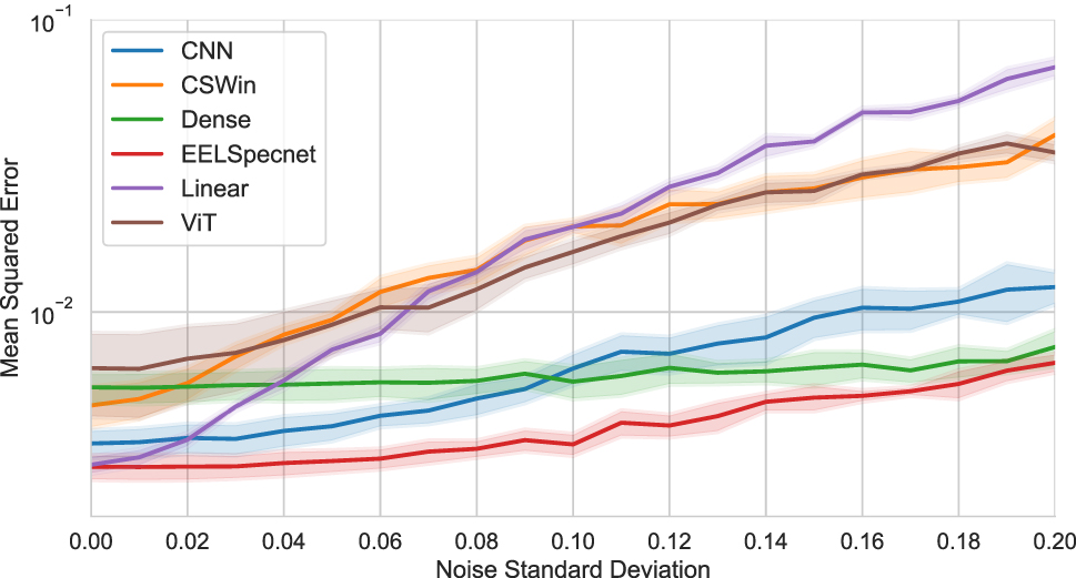
Benchmark results with added noise. The solid lines indicate the mean MSE over all folds, with their standard deviation as the de-saturated area around them.

References

[1] M. Pirzada and Z. Altintas, “Recent progress in optical sensors for biomedical diagnostics,” Micromachines, vol. 11, no. 4, p. 356, 2020. https://doi.org/10.3390/mi11040356.Search in Google Scholar PubMed PubMed Central
[2] M. I. Ahmad Asri, M. Nazibul Hasan, M. R. A. Fuaad, Y.Md. Yunos, and M. S. M. Ali, “Mems gas sensors: a review,” IEEE Sens. J., vol. 21, no. 17, pp. 18381–18397, 2021. https://doi.org/10.1109/jsen.2021.3091854.Search in Google Scholar
[3] C. Prakash, L. P. Singh, A. Gupta, and S. K. Lohan, “Advancements in smart farming: a comprehensive review of IoT, wireless communication, sensors, and hardware for agricultural automation,” Sens. Actuators A: Phys., vol. 362, 2023, p. 114605. https://doi.org/10.1016/j.sna.2023.114605.Search in Google Scholar
[4] S. De Alwis, Z. Hou, Y. Zhang, M. H. Na, B. Ofoghi, and A. Sajjanhar, “A survey on smart farming data, applications and techniques,” Comput. Ind., vol. 138, 2022, p. 103624. https://doi.org/10.1016/j.compind.2022.103624.Search in Google Scholar
[5] W.-H. Su, “Advanced machine learning in point spectroscopy, RGB- and hyperspectral-imaging for automatic discriminations of crops and weeds: a review,” Smart Cities, vol. 3, no. 3, pp. 767–792, 2020. https://doi.org/10.3390/smartcities3030039.Search in Google Scholar
[6] A. Ashapure, J. Jung, A. Chang, S. Oh, M. Maeda, and J. Landivar, “A comparative study of RGB and multispectral sensor-based cotton canopy cover modelling using multi-temporal UAS data,” Remote Sens., vol. 11, no. 23, p. 2757, 2019. https://doi.org/10.3390/rs11232757.Search in Google Scholar
[7] J. Zhang, X. Zhu, and J. Bao, “Solver-informed neural networks for spectrum reconstruction of colloidal quantum dot spectrometers,” Opt. Express, vol. 28, no. 22, pp. 33656–33672, 2020. https://doi.org/10.1364/oe.402149.Search in Google Scholar PubMed
[8] J. Zhang, X. Zhu, and J. Bao, “Denoising autoencoder aided spectrum reconstruction for colloidal quantum dot spectrometers,” IEEE Sens. J., vol. 21, no. 5, pp. 6450–6458, 2021. https://doi.org/10.1109/jsen.2020.3039973.Search in Google Scholar
[9] C.-C. Chang and H.-N. Lee, “On the estimation of target spectrum for filter-array based spectrometers,” Opt. Express, vol. 16, no. 2, pp. 1056–1061, 2008. https://doi.org/10.1364/oe.16.001056.Search in Google Scholar PubMed
[10] J. Zhang, R. Su, Q. Fu, W. Ren, F. Heide, and Y. Nie, “A survey on computational spectral reconstruction methods from RGB to hyperspectral imaging,” Sci. Rep., vol. 12, 2022, no. 1, p. 11905. https://doi.org/10.1038/s41598-022-16223-1.Search in Google Scholar PubMed PubMed Central
[11] U. Kurokawa, B. I. Choi, and C.-C. Chang, “Filter-based miniature spectrometers: spectrum reconstruction using adaptive regularization,” IEEE Sens. J., vol. 11, no. 7, pp. 1556–1563, 2011. https://doi.org/10.1109/jsen.2010.2103054.Search in Google Scholar
[12] P. Wang and R. Menon, “Computational spectroscopy via singular-value decomposition and regularization,” Opt. Express, vol. 22, no. 18, pp. 21541–21550, 2014. https://doi.org/10.1364/oe.22.021541.Search in Google Scholar
[13] S. Junger, N. Verwaal, R. Nestler, and D. Gäbler, “Integrierte Multispektralsensoren in CMOS-Technologie,” in Mikrosystemtechnik Kongress München, 2017.Search in Google Scholar
[14] A. Stefani, et al.., “Investigation of the influence of the number of spectral channels in colorimetric analysis,” in 2021 Conference on Lasers and Electro-Optics Europe and European Quantum Electronics Conference, Munich, Germany, 2021, pp. 1–1. https://doi.org/10.1109/CLEO/Europe-EQEC52157.2021.9542450.Search in Google Scholar
[15] S. Yokogawa, S. P. Burgos, and H. A. Atwater, “Plasmonic color filters for cmos image sensor applications,” Nano Lett., vol. 12, no. 8, pp. 4349–4354, 2012. https://doi.org/10.1021/nl302110z.Search in Google Scholar PubMed
[16] A. Kobylinskiy, et al.., “Substantial increase in detection efficiency for filter array-based spectral sensors,” Appl. Opt., vol. 59, no. 8, pp. 2443–2451, 2020. https://doi.org/10.1364/ao.382714.Search in Google Scholar PubMed
[17] S. M. Shayan Mousavi, A. Pofelski, and G. Botton, “EELSpecNet: deep convolutional neural network solution for electron energy loss spectroscopy deconvolution,” Microsc. Microanal., vol. 27, no. S1, pp. 1626–1627, 2021. https://doi.org/10.1017/s1431927621005997.Search in Google Scholar
[18] O. Ronneberger, P. Fischer, and T. Brox, “U-Net: convolutional networks for biomedical image segmentation,” in Medical Image Computing and Computer-Assisted Intervention – MICCAI 2015, Nassir Navab, Joachim Hornegger, W. M. Wells, and A. F. Frangi, Eds., Cham, Springer International Publishing, 2015, pp. 234–241.10.1007/978-3-319-24574-4_28Search in Google Scholar
[19] Y. Cai, et al.., “Mask-guided spectral-wise transformer for efficient hyperspectral image reconstruction,” in 2022 IEEE/CVF Conference on Computer Vision and Pattern Recognition (CVPR), Los Alamitos, CA, USA, IEEE Computer Society, 2022, pp. 17481–17490.10.1109/CVPR52688.2022.01698Search in Google Scholar
[20] M. Tong, X. Jing, Z. Yan, and W. Pedrycz, “Attention is all you need,” in 31st Conference on Neural Information Processing Systems (NIPS 2017), 2017.Search in Google Scholar
[21] A. Dosovitskiy, et al.., “An image is worth 16x16 words: transformers for image recognition at scale,” in International Conference on Learning Representations, 2021.Search in Google Scholar
[22] Y. Bai, J. Mei, A. L. Yuille, and C. Xie, “Are transformers more robust than CNNs?” in Advances in Neural Information Processing Systems, vol. 34, M. Ranzato, A. Beygelzimer, Y. Dauphin, P. S. Liang, and J. Wortman Vaughan, Eds., Curran Associates, Inc, 2021, pp. 26831–26843.Search in Google Scholar
[23] H. Zhu, B. Chen, and C. Yang, Understanding Why ViT Trains Badly on Small Datasets: An Intuitive Perspective, 2023. https://arxiv.org/abs/2302.03751.Search in Google Scholar
[24] J. Maurício, I. Domingues, and J. Bernardino, “Comparing vision transformers and convolutional neural networks for image classification: a literature review,” Appl. Sci., vol. 13, no. 9, p. 5521, 2023. https://doi.org/10.3390/app13095521.Search in Google Scholar
[25] X. Dong, et al.., “Cswin transformer: a general vision transformer backbone with cross-shaped windows,” in IEEE/CVF Conference on Computer Vision and Pattern Recognition, Los Alamitos, CA, USA, IEEE Computer Society, 2021, pp. 12114–12124.10.1109/CVPR52688.2022.01181Search in Google Scholar
[26] Roscolux, “Roscolux filter swatchbook,” Available at: https://www.edmundoptics.com/f/roscolux-color-filter-swatchbook/12186 Accessed: Apr. 10, 2024.Search in Google Scholar
[27] P. Menz, A. Backhaus, and U. Seiffert, “Transfer learning for transferring machine-learning based models among various hyperspectral sensors,” in European Symposium on Artificial Neural Networks, Computational Intelligence and Machine Learning (ESANN 2019), ESANN, 2019.Search in Google Scholar
© 2024 the author(s), published by De Gruyter, Berlin/Boston
This work is licensed under the Creative Commons Attribution 4.0 International License.
Articles in the same Issue
- Frontmatter
- Editorial
- Measurement systems and sensors with cognitive features III
- Research Articles
- Opportunities of artificial intelligence in the field of calibration services
- Neuronale Netze zur Startwertschätzung bei der Identifikation piezoelektrischer Materialparameter