
Discrepancies in walking speed measurements post-bed-rest: a comparative analysis of real-world vs. laboratory assessments
-
Marcello Grassi
 ,
Ramona Ritzmann
,
Fiona Von Der Straten
,
Jonas Böcker
,
Uwe Mittag
,
Ramona Ritzmann
,
Fiona Von Der Straten
,
Jonas Böcker
,
Uwe Mittag


Abstract
Objectives
Understanding differences between real-world walking speed (RWS) and laboratory-measured walking speed (LWS) is crucial for comprehensive mobility assessments, especially in context of prolonged immobilization. This study aimed to investigate disparities in walking speed following a 60-day bed-rest period.
Methods
In 11 male participants, RWS was continuously monitored using a tri-axial accelerometer worn on the waist, while LWS was assessed via a 10-m walk test at preferred speed, on three different study days after immobilization. Statistical analyses included Bland–Altman and Pearson’s correlation to evaluate agreement between RWS and LWS, alongside paired-sample t-tests and univariate linear regression models to assess significance of differences and temporal effects on gait speed.
Results
Results of Bland-Altman analysis showed no agreement between RWS and LWS (mean difference 0.77 m/s) and nonsignificant correlation (r=0.19, p-value=0.3). Paired-sample t-tests indicated significantly lower RWS compared to LWS for all study days (p-value <0.001). Univariate linear regression models demonstrated a significant effect of test day on RWS (p-value <0.001) but not on LWS (p-value=0.23).
Conclusions
These findings emphasize the importance of integrating both assessments to capture comprehensive mobility changes following prolonged periods of inactivity. Particularly significant is that RWS is constantly lower than LWS, with the former being more representative as it reflects what normally participants would do when not under observation. Lastly, understanding discrepancies between RWS and LWS would allow for more appropriate rehabilitation programs to speed up recovery while simultaneously keeping the rehabilitation safe and tailored.
Introduction
Gait speed is an important well-recognized parameter that reflects mobility and the overall well-being of an individual, as well as being an indicator of physical functioning, cognitive impairment [1], disability, falls and mortality 2], [3], [4], [5. Slow self-selected walking speed is associated with a lower quality of life [6], symptoms of depression [7], higher healthcare utilization [8] and higher mortality rate [9]. The role of gait speed is also linked to the assessment of the recovery process after surgery [10] and after experimental bed-rest 11], [12], [13. Due to its versatility in predicting different outcomes, as well as the relatively low cost and ease to administer, it has been named “the sixth vital sign” by Middleton [4].
However, in recent years it became evident that self-selected walking speed in a controlled environment (e.g., laboratory gait tests) can differ from self-selected walking speed in real-world conditions 14], [15], [16. Even the representativity of laboratory gait tests for real-world behavior has been recently questioned [17] as laboratory-based assessments, often conducted over short distances in controlled settings, may not capture the complexity of real-world ambulation. It was shown that real-world gait assessments using wearables are better at predicting fall risk in older people than clinical gait assessments [18] and undoubtedly offers a more ecologically valid representation of daily mobility patterns [19, 20]. Aforementioned distinctions are paramount when it comes to pathological conditions. Especially in the context of extended bed-rest, it is particularly important to represent gait capacity in realistic scenarios to support a conclusive clinical statement.
Experimental bed-rest studies are widely accepted to simulate the effects of microgravity in space on different physiological systems and therefore, they provide valuable insight in the physiological impact of neuromuscular and coordinative deconditioning. Obviously, that is also relevant to clinical cases of bed-rest. Immobilization by experimental bed-rest leads to a rapid degradation process encompassing most bodily structures, systems, and organs and, hence, a decline in the overall fitness and health status 21], [22], [23. Particularly, gait course analyses after bed-rest of differing lengths showed that preferred walking speed, moderate running speed and spatio-temporal parameters decrease with the duration of bed-rest and results in delayed recovery curves after bed-rest 11], [12], [13. However, clear evidence on the diagnostic differences and specificities of wearable solutions in everyday life compared to laboratory tests is still unclear.
The focus of this work was to study the differences between self-selected laboratory walking speed (LWS) and real-world walking speed (RWS) after 60 days of immobilization by experimental bed-rest. For that purpose, we assessed, in a prospective longitudinal study, gait speed at three equidistant time intervals after the end of bed-rest, named R0, R7 and R13, where the R before the number indicates the recovery phase and the number after the R indicates the day of the recovery phase in which the test was performed (e.g., R7 indicates the seventh day after bed-rest). We hypothesized that LWS and RWS would demonstrate major differences. Furthermore, we investigated whether the effect of time after bed-rest is reflected in LWS and RWS data. The summary of this article is presented in Figure 1.
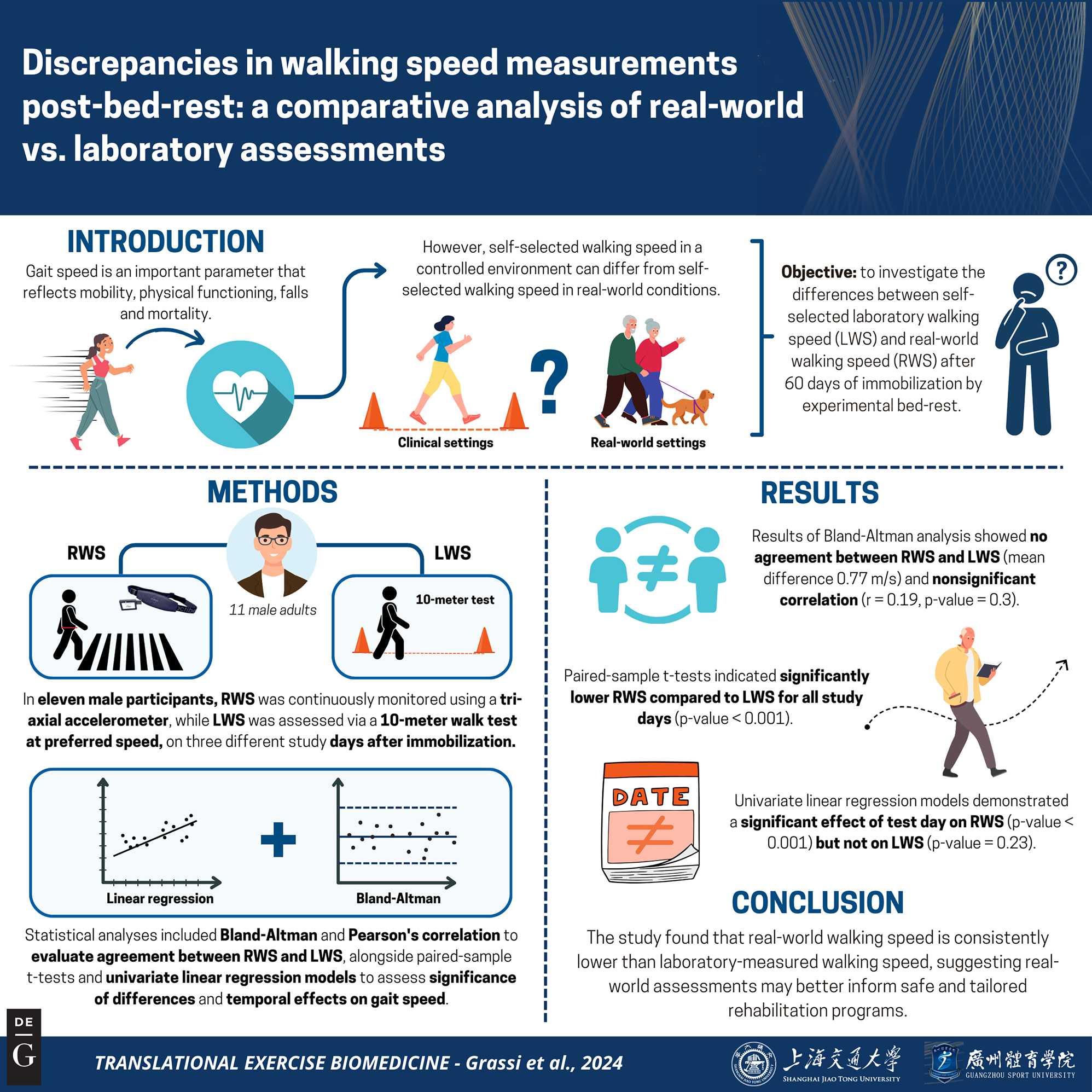
Graphical representation of this study. Key points: (1) Lack of agreement between RWS and LWS: The study found no significant correlation between Real-world Walking Speed (RWS) and Laboratory-measured Walking Speed (LWS), with Bland–Altman analysis showing a mean difference 0f 0.77 m/s, indicating a substantial disparity between the two measures. (2) Consistently lower RWS: RWS was significantly lower than LWS across all study days following the 60-day immobilization period. (3) Temporal effects on RWS: The day of testing significantly influenced RWS, while LWS remained unaffected, suggesting RWS captures gradual changes in mobility better than LWS after prolonged inactivity. Figure created with BioRender.
Materials and methods
Study design
A prospective longitudinal cohort study was performed at the :envihab research laboratory of the Institute of Aerospace Medicine at the German Aerospace Center – Deutsches Zentrum für Luft-und Raumfahrt (DLR) in Cologne, Germany. The bed-rest study took place from February to April 2016 and lasted for 60 consecutive days plus an in-house period of two weeks before and after the bed-rest. Thus, each participant had a two-week Baseline Data Collection (BDC) phase before immobilization, a 60-day 6° head down tilt bed-rest, and another two-week recovery (R) phase. This extended period of 3 months was the second campaign of a bigger study named RSL (Reactive Jumps in a Sledge Jump System as a Countermeasure during Long-Term Bed Rest 2015–2016) (see [24] for more details about the RSL study). During the two two-week phases before and after the immobilization phase, participants were confined to the DLR ward to undergo various measurement procedures (including gait tests).
As a countermeasure against the effect of immobilization by experimental bed rest, seven participants were assigned to undergo 48 training sessions during the bed-rest phase on a Sledge Jump System (SJS) that allows mimicking reactive jumps in a horizonal position at different gravity loads (see [24] for more details on the training sessions and [25] for more information about the training device). On the morning of the first bed-rest day, participants were randomly assigned to either a passive control group that did not perform any training sessions, or to an exercise group, which participated in the scheduled horizontal training sessions.
The study protocol was approved by the ethics committee of the Northern Rhine Medical Association (Ärztekammer Nordrhein) in Düsseldorf, Germany (2014105) and the Federal Office for Radiation Protection (Bundesamt für Strahlenschutz) (Z5-22462/2-2014-032). All participants provided written informed consent before participating.
The study is registered at the German Clinical Trials Register (www.drks.de) under the number DRKS00012946.
Participants
Eleven healthy male participants were randomly assigned into two groups, the control group (CTRL group, n=4; age 31 ± 7.5 years; height 179 ± 2.2 cm; weight 73 ± 8.7 kg) and the exercise group (JUMP group, n=7; age 29.6 ± 6.1 years; height 184 ± 4.8 cm; weight 81.5 ± 4.2 kg). Before being selected as study participants, volunteers had to go through an information session, an interview, two psychological tests and an elaborate medical screening to be sure they were physically and mentally fit for extended period of immobilization (see [24] for further details).
Gait speed measurements
Laboratory gait speed
Gait speed was assessed on a 10-m track [12] at the participants’ preferred gait speed. To assess spatiotemporal characteristics of the locomotor pattern the Optogait system was used (Optogait; Microgate, Bolzano, Italy). The data were extracted at sampling frequency of 200 Hz. Trials were repeated twice and averaged.
Participants were explicitly asked to perform the course at a normal or self-selected pace, meaning they were instructed to walk as they would naturally, without rushing or intentionally slowing down. No time constraints were imposed, nor were they asked to walk as quickly as possible. The goal was to observe their typical walking behavior in a comfortable, real-life scenario. Additionally, the course had a 5-m buffer before and after the start/stop line allowing a flying start and stop to account for acceleration and deceleration phases.
Real-world gait speed
RWS was assessed via a tri-axial accelerometer (actibelt®, Trium Analysis Online GmbH, Munich, Germany) placed on the frontal region below the umbilicus. The device can record acceleration of the body center of mass over the three spatial axes with a sample frequency of 100 Hz. Participants were asked to wear the actibelt® as much as possible during the day to capture all possible walking segments. They were instructed to remove it while taking showers or when sleeping. Wearing time was assessed electronically by the device with a switch that can determine whether the belt buckle is closed. RWS was estimated with the stepwave algorithm [26], which computed the mean speed per each walking step, and subsequently, the daily RWS is derived as the average of these mean speeds. Additionally, the algorithm provides a walking bout index per step, enabling the calculation of walking bout distances. Walking bouts with distances ranging from 8 to 12 m are identified and used in the second section of the analysis presented in this work.
Statistical analysis
Statistical analysis was performed using R Studio v. 4.0.3 (RStudio: Integrated Development Environment for R, RStudio, Inc., Boston, MA).
This study presents two analyses that account for different types of RWS. The first analysis estimates daily RWS using all steps and walking bouts detected by the stepwave algorithm. The second analysis focuses only on walking bouts of approximately 10 m to provide a more consistent comparison. More precisely, the second analysis focused on bouts of length between 8 and 12 m.
For each of the analyses, the following steps have been carried out:
Data distribution of RWS and LWS was assessed with the Shapiro–Wilk test of normality [27] using the R function stats::shapiro.test() and homogeneity of variance between RWS and LWS was tested using the Fligner-Killeen Test of Homogeneity of Variance [28] using the R function stats::fligner.test().
Bland–Altman [29] and Pearson’s product-moment correlation analysis [30] were performed to assess the levels of agreement between the RWS and LWS. Pearson’s product-moment correlation analysis was performed using the R function stats::cor.test(), while the Bland–Altman plot was built using custom R functions.
A paired-sample two-sided t-test was performed to assess whether LWS is significantly greater than RWS using the R function stats::t.test() among all the samples and by study day. The p-values were adjusted for multiple comparisons using the Bonferroni correction [31, 32].
Significance of the effect of test days (R0, R7 and R13) on RWS and LWS was assessed by fitting a univariate linear regression model to the data using the variable of interest (RWS or LWS) as dependent variable and study phase (R0, R7 and R13) as independent variable. The model was fitted by calling the stats::lm() R function. Subsequently, a Tukey Honest Significant Difference test [33] was used as post-hoc test to determine differences between study days. All plots were made using the R library ggplot2, version 3.3.6.
Group information (training or control) was not factored in any of the analyses due to the relatively small number of participants in each group, which precludes a reliable assessment of the outcome.
Data are given in mean ± standard deviations.
Results
All walking bouts
In this section are reported the results coming from the comparison of RWS estimated values using all the walking bouts detected by the stepwave algorithm against the LWS values.
Wearing time
Wearing time of the three-axial accelerometer throughout the three days of measurements was as follows (mean ± SD hours/day): R0: 14.6 ± 2.9, R7: 14.3 ± 4.2 and R13: 15.7 ± 3.5.
Levels of agreement
Bland–Altman showed little to no agreement between the two measurements with a mean difference of 0.77 m/s and the 95 % confidence intervals for the limit of agreements were 0.23 m/s to 1.31 m/s, and no significant correlation (t30=1.05, p-value=0.3, r=0.19).
Level of agreement by study day showed also no agreement between RWS and LWS, with mean difference and 95 % confidence intervals for the limit of agreements (expressed in m/s) of 0.83 [0.29 to 1.38], 0.59 [0.18 to 1] and 0.89 [0.38 to 1.4] for R0, R7 and R13, respectively. Also, the Pearson’s product-moment correlation showed little to no correlation for all three study days (R0: t9=1.71, p-value=0.12; r=0.49; R7: t9=1.27, p-value=0.23, r=0.39; R13: t8=−0.64, p-value=0.54, r=−0.22). Figure 2 and Table 1 present and summarize the results reported in this section.
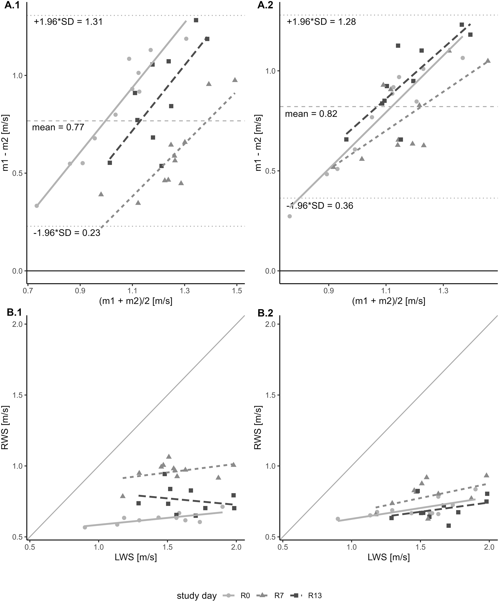
Bland–Altman plot and scatter plot comparing RWS (Real-world Walking Speed) and LWS (Laboratory-measured Walking Speed). Panel A: Bland–Altman plot illustrating the pairwise agreement between two measurements, RWS and LWS, across three study days. The x-axis represents the average of the two measurements, while the y-axis depicts the difference between them. A dashed horizontal line denotes the mean difference between the two measurements. Additionally, two dotted lines indicate the lower and upper limits of agreement. The plot is color-coded with three different shades of grey to differentiate the data points and regression lines corresponding to each of the three study days. Panel A.1 shows comparison of LWS with RWS (all walking bouts). Panel A.2 shows comparison of LWS with RWS (10-m walking bouts). Panel B: Scatter plot showing the relationship between LWS and RWS, both expressed in meters per second (m/s). The x-axis represents LWS, while the y-axis represents RWS. Each data point in the plot corresponds to a measurement obtained from the study. The plot is distinguished by three different shades of grey, each representing data collected on a different study day, together with the respective regression lines. Panel B.1 shows comparison of LWS with RWS (all walking bouts). Panel B.2 shows comparison of LWS with RWS (10-meter walking bouts).
Bland–Altman and Pearson’s product-moment correlation of Real-world walking speed (RWS) and Laboratory-measured walking speed (LWS). Values of the Bland–Altman analysis are given in m/s.
| Study day | |||||
|---|---|---|---|---|---|
| Method | Statistics | Combined | R0 | R7 | R13 |
| All walking bouts | |||||
|
|
|||||
| Bland–Altman | Mean bias | 0.77 | 0.83 | 0.59 | 0.89 |
| Upper limit of agreement | 1.31 | 1.38 | 1 | 1.4 | |
| Lower limit of agreement | 0.23 | 0.29 | 0.18 | 0.38 | |
| Pearson’s product-moment correlation | Pearson’s correlation coefficient | 0.19 | 0.49 | 0.39 | −0.22 |
| Degree of freedom | 30 | 9 | 9 | 8 | |
| t-value | 1.05 | 1.71 | 1.27 | −0.64 | |
| p-value | 0.3 | 0.12 | 0.23 | 0.54 | |
|
|
|||||
| 10-meter walking bouts | |||||
|
|
|||||
| Bland–Altman | Mean bias | 0.82 | 0.76 | 0.77 | 0.95 |
| Upper limit of agreement | 1.28 | 1.26 | 1.17 | 1.35 | |
| Lower limit of agreement | 0.36 | 0.26 | 0.37 | 0.55 | |
| Pearson’s product-moment correlation | Pearson’s correlation coefficient | 0.42 | 0.73 | 0.45 | 0.38 |
| Degree of freedom | 30 | 9 | 9 | 8 | |
| t-value | 2.5 | 3.19 | 1.5 | 1.15 | |
| p-value | 0.02 | 0.01 | 0.17 | 0.28 | |
Moreover, in Figure 2, panel A.1, it can be seen that there is a positive correlation (t30=2.73, p-value=0.01; r=0.45) between the difference of measurements (y-axis) and the mean of measurements (x-axis) suggesting an unequal variance between the two compared measurements. As values of RWS are not normally distributed (W=0.91, p-value=0.012), the Fligner-Killeen Test of Homogeneity of Variances was carried out to compare both variances. The test showed no significant difference between the two variances (RWS variance=0.03, LWS variance=0.07, x 2=1.86, p-value=0.173).
Speed difference between RWS and LWS
The paired-sample t-test showed that RWS (mean=0.78 m/s, SD=0.16 m/s) was significantly lower than LWS (mean=1.55 m/s, SD=0.26 m/s), t31=−15.78, p-value <0.001.
Furthermore, paired-sample t-test executed on the data grouped by study day showed that for all the three study days RWS was significantly lower than LWS (R0: t10=−10.02, p-value <0.001; R7: t10=−9.32, p-value <0.001; R13: t9=−10.88, p-value <0.001 – see Table 2 and Figure 3 for the t-test results). All the p-values were adjusted using the Bonferroni correction for multiple comparisons.
Results of the paired-sample t-test between Laboratory-measured walking speed (LWS) and Real-world walking speed (RWS). Walking speed values are given as mean ± standard deviation and expressed in m/s.
| All samples | R0 | R7 | R13 | |
|---|---|---|---|---|
| All walking bouts | ||||
| Mean ± SD, LWS | 1.55 ± 0.26 m/s | 1.45 ± 0.3 m/s | 1.55 ± 0.23 m/s | 1.65 ± 0.22 m/s |
| Mean ± SD, RWS | 0.78 ± 0.16 m/s | 0.62 ± 0.05 m/s | 0.96 ± 0.07 m/s | 0.76 ± 0.09 m/s |
| Absolute difference (|RWS – LWS|) | 0.77 m/s | 0.83 m/s | 0.59 m/s | 0.89 m/s |
| Degree of freedom | 31 | 10 | 10 | 9 |
| t-statistics | −15.78 | −10.02 | −9.32 | −10.88 |
| p-value | <0.001 | <0.001 | <0.001 | <0.001 |
|
|
||||
| 10-meter walking bouts | ||||
|
|
||||
| Mean ± SD, LWS | 1.55 ± 0.26 m/s | 1.45 ± 0.3 m/s | 1.55 ± 0.23 m/s | 1.65 ± 0.22 m/s |
| Mean ± SD, RWS | 0.73 ± 0.09 m/s | 0.7 ± 0.06 m/s | 0.78 ± 0.1 m/s | 0.7 ± 0.08 m/s |
| Absolute difference (|RWS – LWS|) | 0.82 m/s | 0.76 m/s | 0.77 m/s | 0.95 m/s |
| Degree of freedom | 31 | 10 | 10 | 9 |
| t-statistics | −19.9 | −9.88 | −12.49 | −14.61 |
| p-value | <0.001 | <0.001 | <0.001 | <0.001 |
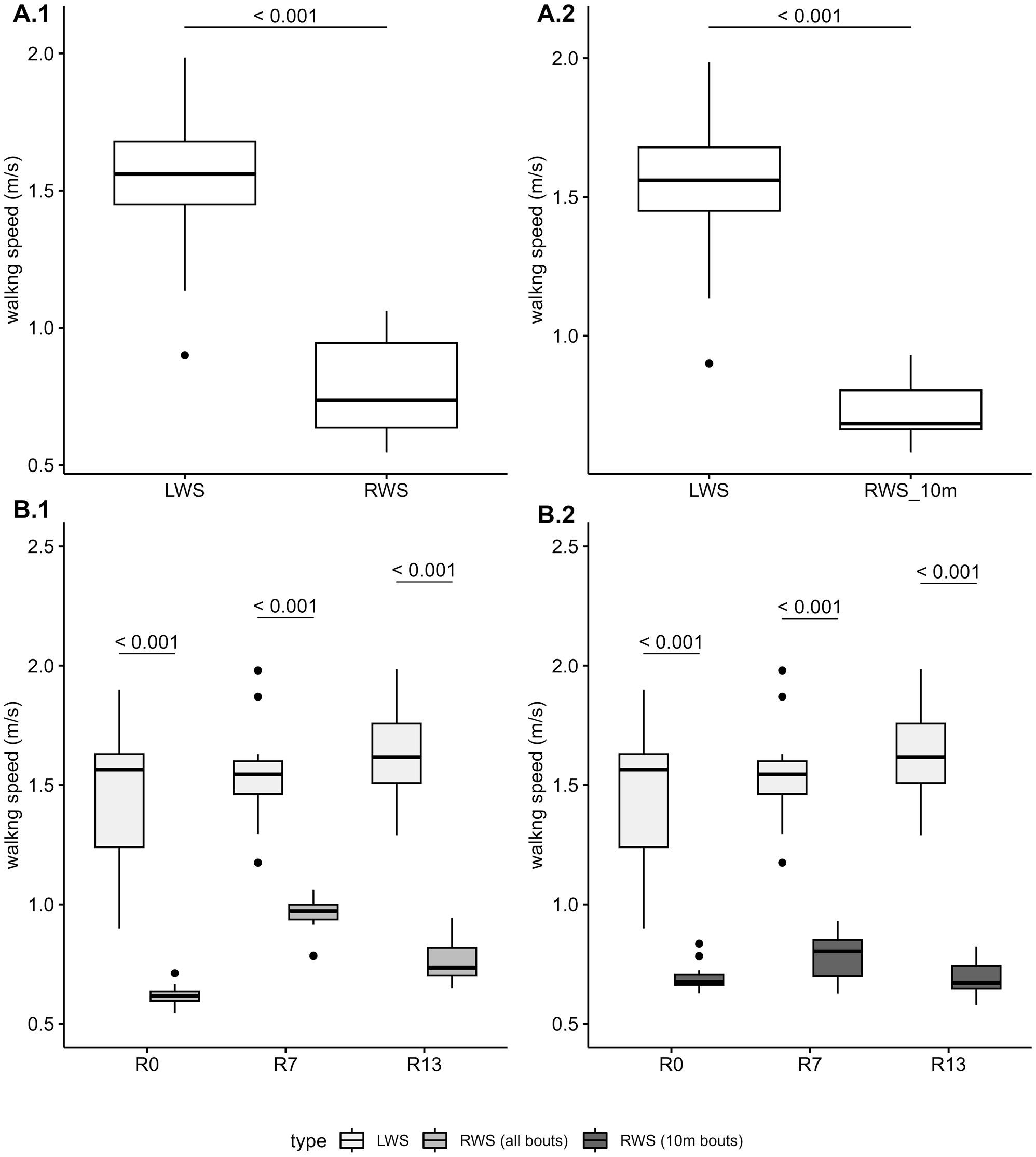
Boxplot illustrating the distribution of LWS (Laboratory-measured Walking Speed) and RWS (Real-world Walking Speed), both expressed in meters per second (m/s). Panels A: Boxplot of the distribution of LWS and RWS for all data points collected. Panels B: Boxplot of the distribution of LWS and RWS by study day (R0, R7 and R13). Panel A.1 and B.1 show values for LWS and RWS (all walking bouts). Panel A.2 and B.2 show values for LWS and RWS (10-m walking bouts).
Effect of test days
The univariate linear regression model fitted on the RWS data showed a significant effect of the test days on RWS (F2=63.01, p-value <0.001). On the other hand, the univariate linear regression model fitted on the LWS data did not show any significant effect of the test days (F2=1.548, p-value=0.23) (see Table 3).
Results of the univariate linear regression analysis on Laboratory-measured walking speed (LWS) and Real-world walking speed (RWS).
| LWS – univariate linear regression model | |||||||
|---|---|---|---|---|---|---|---|
| Coefficients | Model | ||||||
| Name | Estimate | Std. Error | t-value | p-Value | F-statistics | Adjusted R 2 | p-Value |
| Intercept | 1.454 | 0.076 | 19.164 | <0.001 | 1.548 | 0.034 | 0.23 |
| R7 | 0.096 | 0.107 | 0.898 | 0.377 | |||
| R13 | 0.193 | 0.11 | 1.759 | 0.089 | |||
|
|
|||||||
| RWS (all walking bouts) – univariate linear regression model | |||||||
|
|
|||||||
|
Coefficients
|
Model
|
||||||
| Name | Estimate | Std. Error | t-value | p-Value | F-statistics | Adjusted R 2 | p-Value |
|
|
|||||||
| Intercept | 0.62 | 0.022 | 28.8 | <0.001 | 63.01 | 0.8 | <0.001 |
| R7 | 0.34 | 0.03 | 11.16 | <0.001 | |||
| R13 | 0.138 | 0.031 | 4.42 | <0.001 | |||
|
|
|||||||
| RWS (10-m walking bouts) – univariate linear regression model | |||||||
|
|
|||||||
|
Coefficients
|
Model
|
||||||
| Name | Estimate | Std. Error | t-value | p-Value | F-statistics | Adjusted R 2 | p-Value |
|
|
|||||||
| Intercept | 0.7 | 0.03 | 27.69 | <0.001 | 3.99 | 0.16 | 0.03 |
| R7 | 0.09 | 0.04 | 2.46 | 0.02 | |||
| R13 | 0.00 | 0.04 | −0.01 | 1.00 | |||
Subsequent post-hoc testing on the results of the linear regression model performed on the RWS data showed that all the differences tested in the pairwise comparisons (R13-R0, R7-R0 and R7-R13) were significant (p-values=R13-R0: <0.001; R7-R0: <0.001; R7-R13: <0.001 – see Table 4 for a summary of the results of the post-hoc testing, and Figure 4 for a graphical representation of the pairwise differences).
Results of the pairwise Tukey Honest Significant Difference test between the three study days (R0, R7 and R13) across Laboratory-measured walking speed (LWS) and Real-world walking speed (RWS). Difference in walking speed is measured in m/s and 95 % confidence intervals (95 % CI) are given.
| Comparison | Difference (95 % CI) | Adjusted p-Value |
|---|---|---|
| LWS | ||
|
|
||
| R7-R0 | 0.096 (−0.169:0.361) | 0.646 |
| R13-R0 | 0.193 (−0.078:0.465) | 0.201 |
| R13-R7 | 0.097 (−0.175:0.369) | 0.655 |
|
|
||
| RWS (all walking bouts) | ||
|
|
||
| R7-R0 | 0.34 (0.265:0.415) | <0.001 |
| R13-R0 | 0.138 (0.061:0.215) | <0.001 |
| R13-R7 | −0.202 (−0.279:–0.125) | <0.001 |
|
|
||
| RWS (10-m walking bouts) | ||
|
|
||
| R7-R0 | 0.088 (0:0.175) | 0.051 |
| R13-R0 | 0 (−0.09:0.09) | 1.00 |
| R13-R7 | −0.088 (−0.178:0.002) | 0.057 |
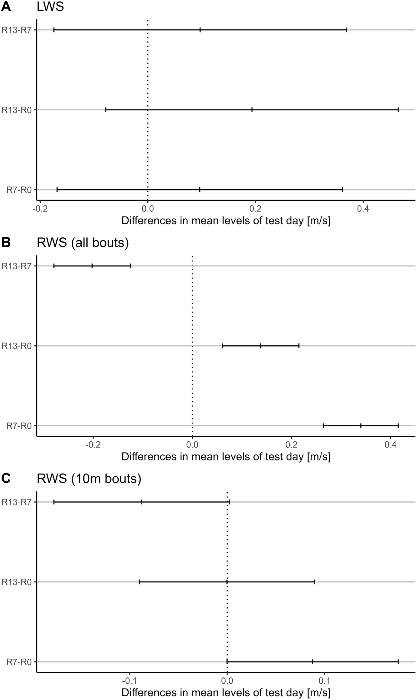
Family-wise confidence level plot illustrating differences in mean levels of test day, expressed in meters per second (m/s) for LWS (Laboratory-measured Walking Speed) and RWS (Real-world Walking Speed). The x-axis displays the differences in mean values between pairs of test days, while the y-axis represents the pairwise comparisons. The mean differences are accompanied by 95 % confidence intervals, providing a measure of uncertainty around the estimated means. This plot aids in visualizing the significance of differences between test days while considering multiple comparisons simultaneously. Panel A: Family-wise confidence level plot for LWS. Panel B: Family-wise confidence level plot for RWS (all walking bouts). Panel C: Family-wise confidence level plot for RWS (10-m walking bouts).
10-meter walking bouts
This section presents the results of the comparison of RWS values, based on walking bouts with length ranging from 8 to 12 m, against LWS values.
Walking bout statistics
The number of bouts covering a distance between 8 and 12 m ranged from a minimum of three bouts per day to a maximum of 53 bouts per day, with an average (±standard deviation) of 20.1 ± 11.05 bouts per day. The distance covered per bout varied from 8.65 to 10.94 m, with an average (±standard deviation) of 9.73 ± 0.36 m. Table 5 provides a summary of the daily number of bouts within this range, along with the corresponding distances covered.
Summary statistics of the Real-world walking speed (RWS) bouts used for the second section of the analysis. Summary statistics are presented for all days (rows Combined) and by study day (rows R0, R7 and R13). Column Qu. 1st refers to the first quantile values. Column Qu. 3rd refers to the third quantile values. Column St. Dev. refers to standard deviation. Values for Number of bouts are given as count. Values for Bout distance is expressed in meters (m).
| Min. | Qu. 1st | Median | Mean | Qu. 3rd | Max | St. Dev. | |
|---|---|---|---|---|---|---|---|
| Number of bouts | |||||||
|
|
|||||||
| Combined | 3 | 12.75 | 20 | 20.12 | 25.75 | 53 | 11.05 |
| R0 | 3 | 7.5 | 13 | 14.73 | 21 | 36 | 10.08 |
| R7 | 8 | 14 | 19 | 21.18 | 22.5 | 53 | 12.37 |
| R13 | 7 | 20.25 | 26.5 | 24.9 | 31.75 | 35 | 8.67 |
|
|
|||||||
| Bout distance, m | |||||||
|
|
|||||||
| Combined | 8.65 | 9.56 | 9.79 | 9.73 | 9.85 | 10.94 | 0.36 |
| R0 | 8.65 | 9.52 | 9.86 | 9.78 | 9.97 | 10.94 | 0.56 |
| R7 | 9.21 | 9.52 | 9.75 | 9.65 | 9.81 | 9.87 | 0.21 |
| R13 | 9.52 | 9.65 | 9.80 | 9.76 | 9.82 | 10.02 | 0.15 |
Levels of agreement
The Bland–Altman analysis revealed minimal to no agreement between the two measurements, with a mean difference of 0.82 m/s. The 95 % confidence intervals for the limits of agreement ranged from 0.36 m/s to 1.28 m/s, and a significant correlation was observed (t30=2.5, p-value=0.02, r=0.42). When analyzed by study day, there was also no agreement between RWS and LWS. The mean difference and 95 % confidence intervals for the limits of agreement (in m/s) were 0.76 [0.26 to 1.26] for R0, 0.77 [0.37 to 1.17] for R7, and 0.95 [0.55 to 1.35] for R13. Additionally, Pearson’s product-moment correlation showed positive correlations across all three study days: R0 (t9=3.19, p-value=0.01; r=0.73), R7 (t9=1.5, p-value=0.17, r=0.45) and R13 (t8=1.15, p-value=0.28, r=0.38). Figure 2 and Table 1 illustrate and summarize the results discussed in this section.
In Figure 2, panel A.2, a positive correlation can be observed between the measurement differences (y-axis) and the mean of the measurements (x-axis), with t30=7.39, p-value <0.001; r=0.8. This suggests unequal variance between the two measurements being compared. Since the RWS values are not normally distributed (W=0.92, p-value=0.024), the Fligner-Killeen Test for Homogeneity of Variances was performed to compare the variances. The test revealed a significant difference between the two, with RWS variance=0.01 and LWS variance=0.07 (x2=9.42, p-value=0.002).
Speed difference between RWS and LWS
The paired-sample t-test indicated that RWS (mean=0.73 m/s, SD=0.09 m/s) was significantly lower than LWS (mean=1.55 m/s, SD=0.26 m/s), t31=−19.9, p-value <0.001. Additionally, when the data were grouped by study day, the paired-sample t-tests showed that RWS was significantly lower than LWS across all three study days: R0 (t10=−9.88, p-value <0.001), R7 (t10=−12.49, p-value <0.001), and R13 (t9=−14.61, p-value <0.001). The p-values were adjusted using the Bonferroni correction for multiple comparisons. Refer to Table 2 and Figure 3 for detailed t-test results.
Effect of test days
The univariate linear regression model applied to the RWS data revealed a significant effect of test days on RWS (F2=3.994, p-value=0.03). In contrast, the model fitted to the LWS data did not show any significant effect of test days (F2=1.548, p-value=0.23) (see Table 3). Post-hoc analysis of the RWS linear regression results indicated that none of the pairwise comparisons (R13-R0, R7-R0 and R13-R7) were not statistically significant: R13-R0 (mean [95 % CI]: 0 [-0.09:0.09], p-value = 1), R7-R0 (mean [95 % CI]: 0.088 [0:0.175], p-value=0.051) and R13-R7 (mean [95 % CI]: −0.088 [-0.178:0.002], p-value=0.057). Refer to Table 4 for a summary of the post-hoc results and Figure 4 for a graphical representation of the pairwise differences.
Discussion
This study provides an important insight into gait assessment within the context of physical impairments, delineating between two distinct methods of assessing gait speed. Results from the Bland–Altman analysis indicates a lack of agreement between the two measurements, with LWS being, on average, greater than RWS by approximately 0.77 m/s when accounting for all the walking bouts, and 0.82 m/s when comparing against 10-m-long walking bouts. Notably, as depicted in Figure 2, panel B.1 and B.2, this discrepancy persisted across all participants and study days. Pearson’s correlation analysis showed minimal correlation between RWS and LWS across all walking bouts. However, a positive correlation (r=0.42) emerged when comparing LWS with the 10-m-long RWS walking bouts, particularly on day R0 (r=0.79, p=0.01). This suggests that on the first day after bed rest, patients who walked slower during the gait test also tended to walk slower during unsupervised 10-m bouts. On test days R7 and R13, the correlation with LWS values weakened (r=0.45 and r=0.38, respectively), indicating an increasing gap between patients’ performance in the supervised test (can-do) and their behavior during unsupervised walking (do-do). Combined, it becomes evident that walking in a controlled laboratory settings differs significantly from everyday ambulation.
Additionally, the variances of LWS and RWS (10-m bouts) were statistically different (p-value=0.002), which complicates the interpretation of the Bland–Altman analysis [34]. This variance difference implies that the bias and limits of agreement are dependent on the range of values used, making the results less generalizable for future applications. However, as the aim of the current work was to understand whether there were discrepancies in the observed walking speed values, and not to find or establish thresholds or rules to consider when performing gait tests and assessing Real-world Walking speed, the Bland–Altman analysis can be considered appropriate for the current context. Despite the variance differences, the method effectively highlights the level of agreements between the two measures, fulfilling the primary objective of identifying discrepancies without requiring strict generalizability across varying conditions.
Many factors can be attributed to the observed difference. Research by Hillel et al. [35] suggests that typical walking in natural environments more closely resembles dual-task walking in a controlled environment. Hillel et al. [35] investigated five commonly used spatial-temporal features of gait quality, including gait speed, in three different settings: in-lab usual walking gait speed, in-lab dual-tasking gait speed and daily-living gait speed. Comparing the gait measurements for the three different settings for a cohort of 150 people revealed that in-lab usual walking gait speed does not agree with measures obtained during daily-living, being significantly faster than daily-living walking speed. Even in-lab dual-tasking gait speed measures, which are overall closer to daily-living gait speed, do not mirror gait speed during daily-living. Consequently, Hillel et al. concluded that, generally-speaking, in-lab measures of gait cannot accurately reflect daily-living gait measures. The findings are in line with our results, indicating that in-lab measurements (LWS) of gait speed before and after physical impairment cannot be equated with the daily walking behavior regarding RWS. Hence, LWS and RWS both contain valuable information about a person’s gait characteristics, however, cannot be treated as equal measurements detached from their environmental contexts.
Furthermore, in another study presented by Kawai [36], the authors explored the relationship between daily living walking speed (DWS) and laboratory-measured walking speed (LWS) in a cohort of 90 elderly individuals. They intended to find out whether DWS serves as reliable indicator of physical function and frailty. Participants were asked to carry a smartphone equipped with a global positioning system (GPS) application for measuring their DWS for one month. During regular checkups, participants performed gait tests in a laboratory to measure LWS at normal and maximum pace. Kawai et al. showed that DWS and LWS (both average and maximum measurements) differ from each other with a mean difference of 0.14 m/s and 0.1 m/s, respectively. While these differences are smaller in magnitude compared to those observed in our study (see Table 2 for gait speed differences overview), they may still hold clinical significance, as suggested by previous studies [37, 38]. Indeed, the study of Kawai showed that DWS measures can be associated with physical performance measurements, hence, Kawai et al. conclude that DWS likely reflects the participants’ physical function. Both the study by Kawai et al. as well as the results of our data analysis underscore that RWS and LWS contain different information about a person’s physical functioning. Kawai et al. also highlight the potential of DWS to assess adverse health outcomes in the future as it can be measured over a long period of time and in different situations compared to LWS.
In another study that focused on the robustness of in-laboratory and daily-life gait speed measures [39], the interrelation between laboratory and daily life gait measures was assessed. Gait measures of 189 elderly people in daily life were collected over the course of one year, as well as regular and frequent intervals in a laboratory environment. Calculating the Pearson’s correlations for in-laboratory and daily-life gait speed revealed negligible to low correlations for all investigated time points. Even though overall correlations increased with higher percentiles of daily-life gait speed, the authors only identified a consistent dissonant relationship between in-laboratory and daily-life gait measures. The authors concluded that both types of gait speed measures represent distinct personal features of a population of elderly people. As both RWS as well as LWS are clinically relevant measures, investigating both measures potentially yield more meaningful insights into actual daily-life physical behavior and improve predicting health outcomes.
The present study revealed that only RWS, and not LWS, was affected by the bed-rest. Conclusion that can be made by looking at the effect of time that was statistically significant only for RWS and not LWS, suggesting a decrease of RWS immediately after bed-rest (R0) followed by a recovery at R7 (see Table 3 for summary of univariate linear regression model applied on RWS and LWS). In contrast, previous studies have reported a significant decline and duration-dependent recovery in laboratory gait speed associated with physiological degradation [11, 12, 40], [41], [42. As such changes were absent in the present, well-controlled study, we conclude that the transferability and significance of laboratory measurements for the real movement patterns in the clinical context must be judged very critically and interpreted thoroughly. The findings presented herein support the notion that walking speed assessed in uncontrolled environments is more sensitive to changes compared to that measured in controlled settings. This is supported by Figure 2, panel B.1, where differences in walking speed are discernible along the y-axis (RWS) but not along the x-axis (LWS). However, this observed dissimilarity should not be solely attributed to differences in measurement sensitivity; it may also stem from distinct underlying mechanisms involved in task execution, as proposed by Takayanagi [15] and Hillel [35]. Notably, in Figure 2, panel B.2 are shown the LWS values plotted against the RWS (10-m bouts), and the differences discernible along the y-axes in panel B.1 are not that distinct anymore, with values for R0 and R13 being very similar. This dissimilarity might hint to the fact that the real-world mechanisms involved in the execution of short (∼10 m) walking bouts remained relatively stable across the recovery phase. Lastly, the high wearing time of the tri-axial accelerometer throughout the study period underscores the feasibility and practicality of continuous monitoring of RWS in real-world setting, enhancing the ecological validity of mobility assessment. However, despite the extensive wear time, the limited number of samples makes it difficult to know to what extent the observations can be generalized. Nevertheless, a post-hoc power analysis yielded a power of 1 (for both “RWS all walking bouts” and “RWS 10-m walking bouts”), indicating that the sample size was sufficient to detect significant differences in walking speed, thereby supporting the robustness of the findings despite the small sample size. Furthermore, participants were restricted to move in the DLR wards on 1,000 m2, so the ‘real-world’ walking bouts they could make were limited to the different stations/areas they had to go for e.g., testing/monitoring, etc. Moreover, it cannot be excluded that participants’ RWS may have been influenced by either DLR personnel while walking together to testing stations or DLR’s ward areas, or by others study participants. While it is reasonable to assume that adjustments to walking speed would be made by the DLR personnel to align with participants’ capabilities, mitigating the risk of injury or discomfort, this may not always have been the case when participants from different recovery days (e.g., R3 and R11) walked together for the DLR’s ward. In such instances, it is conceivable that one participant may have had to adapt its RWS to match the other participant’s RWS, potentially introducing bias to RWS values either upwards or downward. Furthermore, participants were instructed to not overdo physical activity on the first days of ambulation after bed-rest as they would become extremely sore from muscle soreness, which might also partially explain why RWS values are generally relatively low throughout the whole recovery phase (usually values of RWS below 0.8 m/s are associated with unfavorable outcomes [4]). Another limitation that may have introduced bias in the comparison is the use of a 5-m flying start and stop in the gait test. This design ensured that the recorded speed reflected only the participants’ steady-state walking, excluding the initial acceleration and final deceleration phases, which would have typically reduced the LWS values. In contrast, RWS values, derived from real-world walking, included both acceleration and deceleration phases when calculating daily averages, leading to generally lower RWS values used in the analysis.
Conclusions
In conclusion, the observed differences between RWS and LWS highlight the complexities of mobility assessment paradigms and the need for comprehensive evaluation methodologies that encompass both laboratory-based and real-world assessments. These findings have significant implications for clinical practice and research, emphasizing the importance of considering contextual factors and temporal variations in mobility measurements.
Acknowledgments
The authors want to thank all participants and personnel from DLR involved in the study that made it possible.
-
Research ethics: This study protocol was reviewed and approved by ethics committee of the Northern Rhine Medical Association (Ärztekammer Nordrhein) in Duesseldorf, Germany, and the Federal Office for Radiation Protection (Bundesamt für Strahlenschutz).
-
Informed consent: Prior to participating in the study, each participant provided written informed consent for the experimental procedures, which received approval from both the ethics committee of the Northern Rhine Medical Association (Ärztekammer Nordrhein) in Duesseldorf, Germany, and the Federal Office for Radiation Protection (Bundesamt für Strahlenschutz). All experiments and methods described herein were conducted in compliance with the guidelines and regulations of the ethic committees that approved the study.
-
Author contributions: MG, FVDS analyzed the data and drafted the manuscript. MG contributed to the data collection and implemented the statistical analysis. RR contributed to the data collection, data analysis and drafted the manuscript. JB reviewed the manuscript. UM contributed to study preparation and data management. EM supervised the study and revised the manuscript. JR participated in study design, study implementation, study preparation and supervised the data analysis. MD participated in the study design and supervised the data analysis. All authors reviewed the manuscript. All authors have accepted responsibility for the entire content of this manuscript and approved its submission.
-
Use of Large Language Models, AI and Machine Learning Tools: None declared.
-
Conflict of interest: The authors declare the following competing interests: MD is employed by Trium Analysis Online GmbH. MD serves as Scientific Director for Sylvia Lawry Centre for Multiple Sclerosis Research e.V. and, together with Trium Analysis Online GmbH has ownership of trademarks/design/patent applications linked to actibelt® technology. MG has a competing non/financial interest as Sylvia Lawry Center for Multiple Sclerosis Research e.V. is providing access to the actibelt® data and related algorithms to pursue a doctoral title. The remaining authors declare no competing interests.
-
Research funding: This study was not supported by any sponsor or funder.
-
Data availability: The datasets used for producing the current work are available in the Open Science Framework repositories rsl2016/rawdata under the following link https://osf.io/uwfk8/?view_only=772e65b5370b4873abfe471e265d1c0c. The code used for producing the current work is available in the Open Science Framework repository rsl2016 under the following link https://osf.io/uwfk8/?view_only=772e65b5370b4873abfe471e265d1c0c.
References
1. Zhou, H, Park, C, Shahbazi, M, York, MK, Kunik, ME, Naik, AD, et al.. Digital biomarkers of cognitive frailty: The value of detailed gait assessment beyond gait speed. Gerontology 2022;68:224–33. https://doi.org/10.1159/000515939.Search in Google Scholar PubMed PubMed Central
2. Verghese, J, Wang, C, Holtzer, R. Relationship of clinic-based gait speed measurement to limitations in community-based activities in older adults. Arch Phys Med Rehabil 2011;92:844–6. https://doi.org/10.1016/j.apmr.2010.12.030.Search in Google Scholar PubMed PubMed Central
3. Abellan van Kan, G, Rolland, Y, Andrieu, S, Bauer, J, Beauchet, O, Bonnefoy, M, et al.. Gait speed at usual pace as a predictor of adverse outcomes in community-dwelling older people an International Academy on Nutrition and Aging (IANA) Task Force. J Nutr Health Aging 2009;13:881–9. https://doi.org/10.1007/s12603-009-0246-z.Search in Google Scholar PubMed
4. Middleton, A, Fritz, SL, Lusardi, M. Walking speed: the functional vital sign. J Aging Phys Activ 2015;23:314–22. https://doi.org/10.1123/japa.23.2.314.Search in Google Scholar
5. Atkinson, HH, Rosano, C, Simonsick, EM, Williamson, JD, Davis, C, Ambrosius, WT, et al.. Cognitive function, gait speed decline, and comorbidities: the health, aging and body composition study. J Gerontol A Biol Sci Med Sci 2007;62:844–50. https://doi.org/10.1093/gerona/62.8.844.Search in Google Scholar PubMed
6. Ekstrom, H, Dahlin-Ivanoff, S, Elmstahl, S. Effects of walking speed and results of timed get-up-and-go tests on quality of life and social participation in elderly individuals with a history of osteoporosis-related fractures. J Aging Health 2011;23:1379–99. https://doi.org/10.1177/0898264311418504.Search in Google Scholar PubMed
7. Brandler, TC, Wang, C, Oh-Park, M, Holtzer, R, Verghese, J. Depressive symptoms and gait dysfunction in the elderly. Am J Geriatr Psychiatr 2012;20:425–32. https://doi.org/10.1097/jgp.0b013e31821181c6.Search in Google Scholar
8. Montero-Odasso, M, Muir, SW, Hall, M, Doherty, TJ, Kloseck, M, Beauchet, O, et al.. Gait variability is associated with frailty in community-dwelling older adults. J Gerontol A Biol Sci Med Sci 2011;66:568–76. https://doi.org/10.1093/gerona/glr007.Search in Google Scholar PubMed
9. Stanaway, FF, Gnjidic, D, Blyth, FM, Le Couteur, DG, Naganathan, V, Waite, L, et al.. How fast does the Grim Reaper walk? Receiver operating characteristics curve analysis in healthy men aged 70 and over. BMJ 2011;343:d7679. https://doi.org/10.1136/bmj.d7679.Search in Google Scholar PubMed PubMed Central
10. Mangione, K, Craik, RL, Lopopolo, R, Tomlinson, JD, Brenneman, SK. Predictors of gait speed in patients after hip fracture. Physiother Can 2008;60:10–18. https://doi.org/10.3138/physio/60/1/10.Search in Google Scholar PubMed PubMed Central
11. Coker, RH, Hays, NP, Williams, RH, Wolfe, RR, Evans, WJ. Bed rest promotes reductions in walking speed, functional parameters, and aerobic fitness in older, healthy adults. J Gerontol A Biol Sci Med Sci 2015;70:91–6. https://doi.org/10.1093/gerona/glu123.Search in Google Scholar PubMed PubMed Central
12. Ritzmann, R, Freyler, K, Kümmel, J, Gruber, M, Belavy, DL, Felsenberg, D, et al.. High intensity jump exercise preserves posture control, gait, and functional mobility during 60 Days of bed-rest: an RCT including 90 Days of follow-up. Front Physiol 2018;9:1713. https://doi.org/10.3389/fphys.2018.01713.Search in Google Scholar PubMed PubMed Central
13. Grassi, M, Von Der Straten, F, Pearce, F, Lee, J, Mider, M, Mittag, U, et al.. Changes in real-world walking speed following 60-day bed-rest. npj Microgravity 2024;10:6. https://doi.org/10.1038/s41526-023-00342-8.Search in Google Scholar PubMed PubMed Central
14. Foucher, KC, Thorp, LE, Orozco, D, Hildebrand, M, Wimmer, MA. Differences in preferred walking speeds in a gait laboratory compared with the real world after total hip replacement. Arch Phys Med Rehabil 2010;91:1390–5. https://doi.org/10.1016/j.apmr.2010.06.015.Search in Google Scholar PubMed
15. Takayanagi, N, Sudo, M, Yamashiro, Y, Lee, S, Kobayashi, Y, Niki, Y, et al.. Relationship between daily and in-laboratory gait speed among healthy community-dwelling older adults. Sci Rep 2019;9:3496. https://doi.org/10.1038/s41598-019-39695-0.Search in Google Scholar PubMed PubMed Central
16. Renggli, D, Graf, C, Tachatos, N, Singh, N, Meboldt, M, Taylor, WR, et al.. Wearable inertial measurement units for assessing gait in real-world environments. Front Physiol 2020;11:90. https://doi.org/10.3389/fphys.2020.00090.Search in Google Scholar PubMed PubMed Central
17. Van Ancum, JM, van Schooten, KS, Jonkman, NH, Huijben, B, van Lummel, RC, Meskers, CGM, et al.. Gait speed assessed by a 4-m walk test is not representative of daily-life gait speed in community-dwelling adults. Maturitas 2019;121:28–34. https://doi.org/10.1016/j.maturitas.2018.12.008.Search in Google Scholar PubMed
18. Brodie, MA, Coppens, MJ, Ejupi, A, Gschwind, YJ, Annegarn, J, Schoene, D, et al.. Comparison between clinical gait and daily-life gait assessments of fall risk in older people. Geriatr Gerontol Int 2017;17:2274–82. https://doi.org/10.1111/ggi.12979.Search in Google Scholar PubMed
19. Lord, S, Galna, B, Rochester, L. Moving forward on gait measurement: toward a more refined approach. Mov Disord 2013;28:1534–43. https://doi.org/10.1002/mds.25545.Search in Google Scholar PubMed
20. Moe-Nilssen, R, Helbostad, JL. Estimation of gait cycle characteristics by trunk accelerometry. J Biomech 2004;37:121–6. https://doi.org/10.1016/s0021-9290(03)00233-1.Search in Google Scholar PubMed
21. Pavy-Le Traon, A, Heer, M, Narici, MV, Rittweger, J, Vernikos, J. From space to Earth: advances in human physiology from 20 years of bed rest studies (1986–2006). Eur J Appl Physiol 2007;101:143–94. https://doi.org/10.1007/s00421-007-0474-z.Search in Google Scholar PubMed
22. Rittweger, J, Beller, G, Armbrecht, G, Mulder, E, Buehring, B, Gast, U, et al.. Prevention of bone loss during 56 days of strict bed rest by side-alternating resistive vibration exercise. Bone 2010;46:137–47. https://doi.org/10.1016/j.bone.2009.08.051.Search in Google Scholar PubMed
23. Buehring, B, Belavy, DL, Michaelis, I, Gast, U, Felsenberg, D, Rittweger, J. Changes in lower extremity muscle function after 56 days of bed rest. J Appl Physiol 2011;111:87–94. https://doi.org/10.1152/japplphysiol.01294.2010.Search in Google Scholar PubMed
24. Kramer, A, Kümmel, J, Mulder, E, Gollhofer, A, Frings-Meuthen, P, Gruber, M. High-intensity jump training is tolerated during 60 Days of bed rest and is very effective in preserving leg power and lean body mass: an overview of the Cologne RSL study. PLoS One 2017;12:e0169793. https://doi.org/10.1371/journal.pone.0169793.Search in Google Scholar PubMed PubMed Central
25. Kramer, A, Ritzmann, R, Gollhofer, A, Gehring, D, Gruber, M. A new sledge jump system that allows almost natural reactive jumps. J Biomech 2010;43:2672–7. https://doi.org/10.1016/j.jbiomech.2010.06.027.Search in Google Scholar PubMed
26. Keppler, AM, Nuritidinow, T, Mueller, A, Hoefling, H, Schieker, M, Clay, I, et al.. Validity of accelerometry in step detection and gait speed measurement in orthogeriatric patients. PLoS One 2019;14:e0221732. https://doi.org/10.1371/journal.pone.0221732.Search in Google Scholar PubMed PubMed Central
27. Shapiro, SS, Wilk, MB. An analysis of variance test for normality (complete samples). Biometrika 1965;52:591–611. https://doi.org/10.2307/2333709.Search in Google Scholar
28. Conover, WJ, Johnson, ME, Johnson, MM. A comparative study of tests for homogeneity of variances, with applications to the outer continental shelf bidding data. Technometrics 1981;23:351–61. https://doi.org/10.2307/1268225.Search in Google Scholar
29. Altman, DG, Bland, JM. Measurement in medicine: the analysis of method comparison studies. J Roy Stat Soc 1983;32:307–17. https://doi.org/10.2307/2987937.Search in Google Scholar
30. Freedman, D, Pisani, R, Purves, R. Statistics: international student edition, 4th ed. New York: WW Norton & Company; 2007.Search in Google Scholar
31. Abdi, H. The Bonferroni and Sidak corrections for multiple comparisons. In: Encyclopedia of measurement and statistic. Thousand Oaks: Sage; 2007.Search in Google Scholar
32. Bonferroni, CE. Teoria statistica delle classi e calcolo delle probabilità. Pubbl Ist Super Sci Economi Commer Firenze 1936:3–62.Search in Google Scholar
33. Keselman, HJ, Rogan, JC. The Tukey multiple comparison test: 1953–1976. Psychol Bull 1977;84:1050–6. https://doi.org/10.1037//0033-2909.84.5.1050.Search in Google Scholar
34. Mansournia, MA, Waters, R, Nazemipour, M, Bland, M, Altman, DG. Bland-Altman methods for comparing methods of measurement and response to criticisms. Global Epidemiol 2021;3:2590–1133. https://doi.org/10.1016/j.gloepi.2020.100045.Search in Google Scholar PubMed PubMed Central
35. Hillel, I, Gazit, E, Nieuwboer, A, Avanzino, L, Rochester, L, Cereatti, A, et al.. Is every-day walking in older adults more analogous to dual-task walking or to usual walking? Elucidating the gaps between gait performance in the lab and during 24/7 monitoring. Eur Rev Aging Phys Act 2019;16:6. https://doi.org/10.1186/s11556-019-0214-5.Search in Google Scholar PubMed PubMed Central
36. Kawai, H, Obuchi, S, Watanabe, Y, Hirano, H, Fujiwara, Y, Ihara, K, et al.. Association between daily living walking speed and walking speed in laboratory settings in healthy older adults. Int Environ Res Public Health 2020;17:2707. https://doi.org/10.3390/ijerph17082707.Search in Google Scholar PubMed PubMed Central
37. Perera, S, Mody, SH, Woodman, RC, Studenski, SA. Meaningful change and responsiveness in common physical performance measures in older adults. J Am Geriatr Soc 2006;54:743–9. https://doi.org/10.1111/j.1532-5415.2006.00701.x.Search in Google Scholar PubMed
38. Kwon, S, Perera, S, Pahor, M, Katula, JA, King, AC, Groessl, EJ, et al.. What is a meaningful change in physical performance? findings from a clinical trial in older adults (the LIFE-P study). J Nutr Health Aging 2009;13:538–44. https://doi.org/10.1007/s12603-009-0104-z.Search in Google Scholar PubMed PubMed Central
39. Rojer, AGM, Coni, A, Mellone, S, Van Ancum, JM, Vereijken, B, Helbostad, JL, et al.. Robustness of in-laboratory and daily-life gait speed measures over one year in high functioning 61- to 70-year-old adults. Gerontology 2021;67:650–9. https://doi.org/10.1159/000514150.Search in Google Scholar PubMed
40. Grassi, M. Using a tri-axial accelerometer to quantify the locomotive patterns before and after 60 days of bed-rest [M.Sc. thesis]. Constance: University of Konstanz; 2016.Search in Google Scholar
41. Floreani, M, Rejc, E, Taboga, P, Ganzini, A, Pišot, R, Šimunič, B, et al.. Effects of 14 days of bed rest and following physical training on metabolic cost, mechanical work, and efficiency during walking in older and young healthy males. PLoS One 2018;13:e0194291. https://doi.org/10.1371/journal.pone.0194291.Search in Google Scholar PubMed PubMed Central
42. Aarden, JJ, Reijnierse, EM, van der Schaaf, M, van der Esch, M, Reichardt, LA, van Seben, R, et al.. Hospital-ADL study group longitudinal changes in muscle mass, muscle strength, and physical performance in acutely hospitalized older adults. J Am Med Dir Assoc 2021;22:839–45. https://doi.org/10.1016/j.jamda.2020.12.006.Search in Google Scholar PubMed
© 2024 the author(s), published by De Gruyter on behalf of Shangai Jiao Tong University and Guangzhou Sport University
This work is licensed under the Creative Commons Attribution 4.0 International License.
Articles in the same Issue
- Frontmatter
- Issue 3: Skeletal muscle, exercise, aging and chronic disease
- Section: Integrated exercise physiology, biology, and pathophysiology in health and disease
- Impact of exercise and fasting on mitochondrial regulators in human muscle
- Effectiveness of aerobic exercise interventions on balance, gait, functional mobility and quality of life in Parkinson’s disease: an umbrella review
- Creatine and strength training in older adults: an update
- Creatine supplementation strategies aimed at acutely increasing and maintaining skeletal muscle total creatine content in healthy, young volunteers
- Section: Physical activity/inactivity and health across the lifespan
- Independent mobility and physical activity among children residing in an ultra-dense metropolis
- Physical activity and cardiometabolic risk factors in sprint and jump-trained masters athletes, young athletes and non-physically active men
- Cross-sectional analysis of blood leukocyte responsiveness to interleukin-10 and interleukin-6 across age and physical activity level
- Section: Exercise and E-health, M-health, AI and technology
- Assessing core body temperature in a cool marathon using two pill ingestion strategies
- Issue 4: Preclinical and clinical approaches to translational exercise biomedicine
- Section: Integrated exercise physiology, biology, and pathophysiology in health and disease
- Nicotinic acid improves mitochondrial function and associated transcriptional pathways in older inactive males
- Exogenous Beta-guanidinopropionic acid administration enhances electromyostimulation-induced mitochondrial biogenesis in rat skeletal muscle
- How exercise shapes the anti-inflammatory environment in multiple sclerosis – a conceptual framework focusing on tryptophan-derived molecules in T cell differentiation
- Section: Personalized and advanced exercise prescription for health and chronic diseases
- Acute effects of high-intensity interval training on microvascular circulation: a case control study in uveal melanoma
- Discrepancies in walking speed measurements post-bed-rest: a comparative analysis of real-world vs. laboratory assessments
- Section: Sports medicine and movement science
- Lower-body strength, power and sprint front crawl performance
- Section: Letter to the editor
- Comment on: “A unique pseudo-eligibility analysis of longitudinal laboratory performance data from a transgender female competitive cyclist”
- Author’s response to “letter to the editor comment on: ‘A unique pseudo-eligibility analysis of longitudinal laboratory performance Data from a transgender female competitive cyclist’” by Lundberg, O’Connor, Kirk, Pollock, and Brown