Analysis of the Number of Tests, the Positivity Rate and Their Dependency Structure During COVID-19 Pandemic
-
Babak Jamshidi
 ,
Hakim Bekrizadeh
,
Hakim Bekrizadeh

Abstract
Recent advances in medical instruments, information technology, and unprecedented data sharing allowed scientists to investigate, trace, and monitor the COVID-19 pandemic faster than any previous outbreak. This extraordinary speed makes COVID-19 a medical revolution that causes some unprecedented analyses, discussions, and models. Modeling the dependence between the number of tests and the positivity rate is one of these new issues. Using four classes of copulas (Clayton, Frank, Gumbel, and FGM), this study is the first attempt tom model the dependency. The estimation of the parameters of the copulas is obtained using the maximum likelihood method. To evaluate the goodness of fit of the copulas, we calculate AIC. The computations are conducted on Matlab R2015b, R 4.0.3, Maple 2018a, and EasyFit 5.6. Findings indicate that at the beginning of a typical epidemic, the number of tests is relatively low and the proportion of positivity is high. As time passes, the number of tests increases, and the positivity rate decreases. The epidemic peaks are occasions that violate the stated general rule –due to the early growth of the number of tests. Also, during both peak and non-peak times, the rising number of tests is accompanied by decreasing the positivity rate. We find that the proportion of positivity is more proportional than the number of tests to the number of infected cases. Therefore, the changes in the positivity rate can be considered a representative of the level of the spreading. Approaching zero positivity rate is a good criterion to scale the success of a healthcare system in fighting against an epidemic. Accordingly, the number and accuracy of tests can play a vital role in the quality level of epidemic data.
Key messages
In a country, increasing the positivity rate is more informative than increasing the number of tests to warn about an epidemic peak.
Approaching zero positivity rate is a good criterion to scale the success of a healthcare system in fighting against an epidemic.
Except for the first half of the epidemic peaks, in a country, the higher number of tests is associated with a lower positivity rate.
1 Introduction
Dr. Li Wenliang, a 34-year-old ophthalmologist, warned his colleagues and set the alarm to the society about a new infection caused by a type of coronavirus in December 2019 in Wuhan, China (Jamshidi et al. 2020). Shortly after his warning, all over the world encountered this epidemic. WHO declared this fast speeding infection (COVID-19) in March 2020 as a pandemic. As of January 20, 2023, over 600 million cases, and around seven million deaths involving COVID-19 have been reported around the world. The epidemic COVID-19 is the most informative pandemic throughout history. These unprecedented recorded data give rise to some unprecedented concepts, relationships, analyses, discussions, and models (Jamshidi et al. 2021).
Modeling the dependence between the number of tests and the proportion of positivity (positivity rate) is one of these new issues. The proportion of positivity is a critical measure because it gives us an indication of how widespread infection is in the area of interest. The proportion of positivity helps public health officials answer questions such as:
What is the current level of SARS-CoV-2 (coronavirus) transmission in the community?
Are we doing enough testing for the people who are getting infected (Dowdy and D’souza 2020)?
According to the ratio nature, the high proportion of positivity is due to the high number of positive tests or the low number of total tests. Based on the first possibility, a higher positivity rate suggests higher transmission and that there are likely more people with coronavirus in the community who have not been tested yet. On the other hand, according to the second possibility, a high percentage of positivity means that more testing should probably be done. Accordingly, for policymakers, the high value for this parameter suggests either it is not a good time to relax restrictions aimed at reducing transmission, or it is a good time to add restrictions to slow the spread of disease (Dowdy and D’souza 2020). In this regard, an analytic report segregated by regions in the UK was presented by the Office for National Statistics (Coronavirus 2021).
This study is the first paper to highlight the importance of availability of the required tests and to model the effect of shortage of tests on the positivity rate. Our motivation is overcoming this ambiguity and giving a clear insight into the real status of the epidemic in the population. We want to emphasize the importance of fluctuations of positivity rate over the study time. We also aim to show the effect of available tests on these fluctuations. To highlight the meaningfulness of the criterion of interest, we use the data of 12 countries and compare them in terms of the other criteria. This study aims to investigate the time series of positivity rates individually and together with the time series of the number of tests. This investigation is conducted in two analytic methods: regional and temporal. The individual analysis is mainly undertaken based on the peaks of the spreading of the pandemic. For the regional aspect, among the 221 countries, we selected 12 countries: the USA, India, the UK, Italy, Iran, the UAE, Bolivia, Guatemala, Nigeria, Australia, South Korea, and South Africa. The reasons for selecting these 12 countries are
They are the top countries in the influential indices (Table 1).
Some of them are widely different from the others in some indices (Table 1).
Their positivity rates are greatly dispersed (Table 2).
The numbers and time of peaks are different about them (Table 3).
Their quality of healthcare systems are of different levels.
Their data, especially about the number of tests are relatively well recorded.
They are selected from all continents: the USA and Guatemala from North America; Bolivia from South America; India, Iran, the UAE, and South Korea from Asia; the UK and Italy from Europe; Nigeria and South Africa from Africa; and Australia from Australia.
The information on the influential indicators of COVID-19 in the 12 countries of interest.
| Country | Total cases | Total deaths | Total tests | Cases per million | Deaths per million | Tests per million | Population |
|---|---|---|---|---|---|---|---|
| USA | 26 M (1) | 429 K (1) | 299 M (1) | 77 K (7) | 1293 (11) | 901 K (19) | 333 M (3) |
| India | 11 M (2) | 154 K (3) | 192 M (2) | 7688 (115) | 111 (104) | 138 K (107) | 1387 M (2) |
| UK | 3647 K (5) | 98 K (5) | 67 M (5) | 54 K (25) | 1438 (5) | 987 K (17) | 68 M (21) |
| Italy | 2467 K (8) | 85 K (6) | 31 M (8) | 41 K (36) | 1415 (7) | 512 K (40) | 60 M (24) |
| Iran | 1373 K (16) | 57 K (9) | 8635 K (20) | 16 K (88) | 678 (43) | 102 K (126) | 85 M (18) |
| UAE | 278 K (43) | 792 (90) | 25 M (12) | 28 K (63) | 80 (117) | 2466 K (5) | 10 M (92) |
| Bolivia | 200 K (53) | 9923 (33) | 514 K (106) | 17 K (84) | 844 (34) | 44 K (150) | 12 M (79) |
| Guatemala | 154 K (67) | 5465 (43) | 738 K (94) | 8519 (112) | 302 (73) | 41 K (153) | 18 M (65) |
| Nigeria | 122 K (76) | 1504 (80) | 1241 K (75) | 582 (180) | 7 (178) | 5939 (194) | 209 M (7) |
| Australia | 29 K (107) | 909 (88) | 13 M (14) | 1121 (163) | 35 (138) | 495 K (41) | 26 M (54) |
| S Korea | 75 K (86) | 1360 (82) | 5284 K (37) | 1500 (155) | 27 (148) | 108 K (121) | 51 M (28) |
| S Africa | 1418 K (15) | 41 K (14) | 7993 K (22) | 24 K (75) | 703 (42) | 137 K (109) | 60 M (25) |
-
The numbers in parentheses indicate the rank of countries among 221 countries in the world. For example, Iran has the 18th population among all countries. The bold numbers display the ranks of the second half of the global ranking. The ranks 111 to 221 are considered the second half. For example, regarding cases per million, India is a country of the second half. The light-highlighted cells show that the country is among the highest quarter of the countries based on the relevant parameter. The darker highlighted cells indicate the country is among the top 5% worldwide. For example, the first row illustrates that except for the criterion of the number of tests per million – where it is among the highest quartile –, the USA is of the top 5% in all indicators.
The properties of the datasets of the countries of interest.
| Country | Lag | Positivity rate | Start | End | Number of days |
|---|---|---|---|---|---|
| USA | 2 | 8 | 27 February 2020 | 27 January 2021 | 334 |
| India | 3 | 6 | 3 March 2020 | 27 January 2021 | 329 |
| UK | 2 | 5 | 21 February 2020 | 25 January 2021 | 338 |
| Italy | 3 | 8 | 19 February 2020 | 27 January 2021 | 339 |
| Iran | 4 | 16 | 1 April 2020 | 26 January 2021 | 303 |
| UAE | 3 | 1 | 11 March 2020 | 26 January 2021 | 318 |
| Bolivia | 5 | 39 | 19 March 2020 | 24 January 2021 | 308 |
| Guatemala | 5 | 21 | 14 March 2020 | 27 January 2021 | 316 |
| Nigeria | 5 | 10 | 17 March 2020 | 27 January 2021 | 313 |
| Australia | 2 | 0.02 | 22 March 2020 | 26 January 2021 | 308 |
| S Korea | 2 | 0.01 | 18 February 2020 | 30 January 2021 | 347 |
| S Africa | 4 | 2 | 14 March 2020 | 30 January 2021 | 320 |
The epidemic peaks of COVID-19 in the countries of interest.
| Country | First peak | Second peak | Third peak |
|---|---|---|---|
| USA | Early April** | Second half of July** | From November to January 2021** |
| India | Middle September*** | - | – |
| UK | Middle April*** | Early November** | Late December*** |
| Italy | Late March** | Early November*** | – |
| Iran | Late March** | Second half of November** | – |
| UAE | Middle May** | January 2021** | – |
| Bolivia | July to August*** | Middle January 2021*** | – |
| Guatemala | – | – | – |
| Nigeria | June to July**# | January 2021***# | – |
| Australia | Late March** | Early August*** | – |
| S Korea | February to March*** | Second half of August** | December*** |
| S Africa | July*** | December and January 2021*** |
-
All the dates belong to 2020. Otherwise, the year is mentioned. (*): Indicated only by the time series of the number of tests. (**): Indicated only by the time series of the proportion of positive tests. (***): Indicated by both time series. (#): After moving average.
Finally, to illustrate the dependency of the number of tests and the positivity rates, we apply copulas.
Sklar introduced the concept of copulas in 1959 (Sklar 1959). A copula – mainly parametric, partially semi-parametric, and rarely non-parametric – is a function that completely describes the dependency structure. It contains all the information to link the marginal distributions to their joint distribution. Accordingly, to obtain a valid multivariate distribution function, it suffices to combine several marginal distribution functions with any candidate for the copula function. Thus, for the purposes of statistical modeling, it is desirable to have a large collection of copulas at one’s disposal. Copula is widely applied in diverse fields, including environmental studies (Corbella and Stretch 2013; Zhang and Singh 2007) finance (Boubaker and Sghaier 2013; Wang et al. 2014), hydrology (Bekrizadeh et al. 2013), and medical studies (Bekrizadeh 2021; Bekrizadeh and Jamshidi 2017; Bekrizadeh et al. 2017; Chatrabgoun et al. 2020; Li and Fang 2012; Roman et al. 2012; Wienke 2011).
2 Data
The main data sources of the paper are the websites Worldometers (Worldometer website) and Our World in Data (Hasell et al. 2020). We summarize and illustrate all the relevant information about the 12 countries in three (twelve-row) tables and three (twelve-partitioned) figures created on Matlab R2015b.
Table 1 includes the key general indicators up to January 25, 2021. It is worth saying that the total indicators or even per-million indicators do not determine the quality of healthcare systems because there are observable underreported statistics about the countries Bolivia, Guatemala, Nigeria, Iran, and even India. On the other hand, we consider the indicator of the number of tests per one million (the 7th column of Table 1) as a criterion representing the level of facilities, therefore the quality of healthcare systems. Based on the information about this criterion, we define the lags (the distance between the test and diagnosis) for the different healthcare systems.
Table 2 represents the underlying properties of any country. As mentioned before, lag is the difference between the time of testing and the time of receiving the results of the tests, positive or negative, in days. The more facilities a healthcare system has, the more tests that system can do – therefore the lower positivity rate it has. Also, the more facilities a healthcare system has, the lower distance is between the tests and results. Based on the concept of lag, we pair the number of tests on the
Generally, during an epidemic wave, the number of new infected individuals increases rapidly to an epidemic peak and then falls more gradually until the epidemic wave is over, and the number of new cases be stabilized. Roughly speaking, the epidemic peaks are the – neighborhood of – time points that corresponds the local maximum of the number of newly infected cases.
3 Methods
3.1 Change Point Detection
We define the epidemic peak as the time neighborhood – or the time point – that
This definition is derived from the definition of outlier in regression analysis. These epidemic peaks are local maximums. In addition, it is noticeable that the distance between two successive epidemic peaks must be at least one month. According to this definition, the peaks of Table 3 are obtained for the countries of interest. It is remarkable that except for the peaks of Bolivia – which are almost the same –, the later waves are more acute than previous ones. We must add this point that the more acute peak means the more number of new confirmed cases, therefore the more intense spreading. Finally, it is possible that because of the lack of information at the beginning, this definition misses the epidemic peaks in the initial days.
Mathematically and logically, the number of positive tests (confirmed cases) is affected by the number of tests and positivity rate. The number of cases equals the number of tests multiplied by the positivity rate. Therefore, the increment of the number of cases (as a multiplication) equals the sum of these two:
The number of tests multiplied by the increment of positivity rate, and
The positivity rate multiplied by the increment of the number of tests.
Consequently, the intense changes in the count of cases are due to at least a remarkable change in one of these multiplications. About the countries with a regular increase in the number of tests like the USA, the increment of the proportion of positivity plays the principal role in the peaks.
Table 3 shows that the proportion of positivity is significantly better than the frequency of tests to indicate the peaks of the pandemic. The positivity rate is more associated with the number of cases than the number of tests (90% vs 45%). After moving average, these proportions reach 100% and 50%, respectively.
Countries of the southern and northern hemispheres faced a peak around July and November, respectively, possibly due to falling temperatures.
Figures 1, 2, and 3 consist of 12 subfigures, each of them belonging to one country. The arrangement of the subfigures in all three figures is identical. The horizontal axes in Figures 1 and 3 represent time in days from the start to the end of the period of study for the studied countries (the fourth and fifth columns of Table 2). The vertical axis of Figures 1 and 2 display the number of new tests – conducted on that day – and the proportion of positive tests – reported that day –, respectively. Figure 3 is the plot of the joint distribution of the number of tests on a day and the proportion of positivity on

The time series of the number of new tests (daily) in the 12 countries. The peaks of the number of tests coincide with the epidemic peaks of COVID-19 in different countries. USA (r1 c1), India (r1 c2), UK (r2 c1), Italy (r2 c2), Iran (r3 c1), UAE (r3 c2), Bolivia (r4 c1), Guatemala (r4 c2), Nigeria (r5 c1), Australia (r5 c2), South Korea (r6 c1), and South Africa (r6 c2). r: row & c: column.

The time series of the positivity rate (daily) in the 12 countries. The peaks of the positivity rate coincide with the epidemic peaks of COVID-19 in different countries. USA (r1 c1), India (r1 c2), UK (r2 c1), Italy (r2 c2), Iran (r3 c1), UAE (r3 c2), Bolivia (r4 c1), Guatemala (r4 c2), Nigeria (r5 c1), Australia (r5 c2), South Korea (r6 c1), and South Africa (r6 c2). r: row & c: column.

Scatterplots of the relationship between the number of tests and the positivity rate. Generally, as the number of new tests increases, the positivity rate falls. USA (r1 c1), India (r1 c2), UK (r2 c1), Italy (r2 c2), Iran (r3 c1), UAE (r3 c2), Bolivia (r4 c1), Guatemala (r4 c2), Nigeria (r5 c1), Australia (r5 c2), South Korea (r6 c1), and South Africa (r6 c2).
Figure 1 shows that the peaks of the number of tests coincide with the epidemic peaks of COVID-19 in different countries. For example, in the USA, there are two peaks of the number of tests simultaneous with the second and the third epidemic peaks – mentioned in Table 3. Also, it is obvious that Bolivia has experienced two peaks for the number of tests around 150th and 300th days – from March 19, 2020 – which coincide with the epidemic peaks in Table 3.
The USA, the UK, and the UAE experienced some regularly rising time series. Except for some overruns in epidemic peaks, the patterns of Italy and South Africa are increasing too. The number of tests in Guatemala is increasing, accompanied by an increasing fluctuation. Owing to the restriction by the limited capacity of tests, Iran and Nigeria followed a stepwise trend. Apart from their peaks – one for each of them –, the plots of Australia and South Korea are stationary. In the case of Bolivia, the time series is proportional to the peaks. India is the only country whose time series is initially increasing, then stable, and after that decreasing. Generally, the counties have an increasing trend.
Figure 4 gives us a classification about the countries from the viewpoint of the number of tests: 1. The USA, 2. India, 3. The UK, 4. Italy, Australia, and the UAE, 5. South Korea, South Africa, and Iran, and 6. Nigeria, Guatemala, and Bolivia.

The time series of the number of new tests (daily) in the 12 countries. The USA, India, and the UK had the greatest number of tests.
Figure 2 illustrates the time series of the positivity rate of the tests (the ratio of the number of positive tests on a day to the number of taken tests on
Figure 5 illustrates a classification of the countries based on the positivity rate: 1. Nigeria, Guatemala, and Bolivia, 2. South Africa, and Iran, 3. The USA, India, the UK, and Italy, and 4. Australia, the UAE, and South Korea.
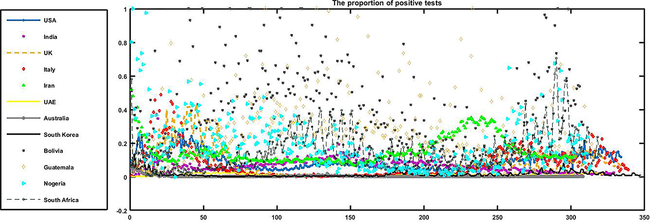
The time series of the positivity rate (daily) in the 12 countries. Nigeria, Guatemala, and Bolivia had the greatest positivity rates among the 12 countries.
The horizontal and vertical axes of Figure 3 display the number of new tests and the proportion of positivity of them, respectively. Generally, as the number of new tests increases, the positivity rate falls. Since the epidemic peaks are opposing this general rule, it is not very clear to see the opposite direction of the changes. Guatemala, due to lack of epidemic peak, is a good example of this diversely proportional relationship.
If the reason for an increase be the rising number of tests, we expect not to return the previous channel in short term. In addition, the positivity rate does not undertake a remarkable change. On the other hand, it is normal to assume that entering a peak is accompanied by increasing the number of negative tests as well. Consequently, the lack of the growth of negative test results (rising the positivity rate while continuing the previous trend for the frequency of tests) is only reasonable if at least one of the factors of tests accuracy, testing policy, or the viewpoint of the population were changed around that time. Otherwise, there are a remarkable number of un-reported cases belonging the peak. It is noticeable that this company of risings causes the observed acceleration in growth regarding epidemic peaks.
3.2 Copulas
3.2.1 Definition
Copulas are functions that connect multivariate distribution functions to their one-dimensional marginal distribution functions -uniform on the interval [0, 1]. Mathematically speaking, if H is a bivariate distribution function with margins F(X) and G(Y), there must exist a copula C such that H θ (X,Y) = C(F(X),G(Y);θ)), where θ is introduced as the dependence parameter (Sklar 1959). Accordingly, Copula is mostly defined as a function C:[0,1]2 → [0,1] that satisfies boundary conditions:
Eventually, for twice differentiable function C, 2-increasing property (P2) can be replaced by the condition
where C(s,t) is the so-called copula density. A copula C is symmetric if C(s,t) = C(t,s), for every
FGM copula (Farlie 1960; Morgenstern 1956);
Clayton copula (Clayton 1978);
Frank copula (Genest 1987);
Gumbel copula (Gumbel 1960);
The parameters of the marginal and copula distributions are estimated using the maximum likelihood method. The computations and illustrations regarding copula theory are conducted in software Maple, R 4.0.3, Maple 2018a, and EasyFit 5.6.
3.2.2 Copula Vs Correlation Coefficient
Measures of dependence are common instruments to summarize a complicated dependence structure in the bivariate case. Pearson’s, Spearman’s rho, and Kendall’s tau correlation coefficients are common statistical measures of dependence structure (Kendall 1970; Pearson 1895; Spearman 1904). The correlation comes in trouble when the random variables are not elliptically distributed. The performance of the copula does not depend on the fact that if you are dealing with elliptical distributions or not. The Pearson’s linear correlation measure (−1 ≤ r ≤ 1) is the most popular and well-known measure between pairwise random variables. Despite its simplicity and plain rationale, Embrechts et al. (2001) noted that ρ is simply a measure of the dependency of elliptical distributions, such as the binormal distribution (the marginals are normally distributed, linked by the Gaussian copula). Moreover, ρ measures a linear relationship itself and does not capture a non-linear one on its own, as noted in (Priest 2003). These properties constitute obvious limitations for modeling the dependency structure. In addition, copulas could be useful to define nonparametric measures of dependence between random variables. Since the values of Kendall’s tau are easy to calculate, this measure is used for observation dependencies. If F(X) and G(Y) are continuous then C(s,t) is unique, else C(s,t) is uniquely determined on the range of F(X) × range of G(Y).
One standard non-parametric dependence measures Kendall’s τk is expressed in the copula form as:
The parameter copula is estimated and the relationship between parameter copula and τk is given in the last column of Table 4. The parameter copula in each case measures the degree of dependence and controls the association between two variables. When the parameter approaches 0 there is no dependence, and if the parameter tends to infinity there is a perfect dependence. Schweizer and Wolff (1981) showed that the dependence parameter copula, which characterizes each family of copulas can be related to Kendall’s τk. Therefore, copulas allow modeling both linear and non-linear dependence. Using copulas, regardless of marginal distributions, can model extreme endpoints.
Kendall’s tau of copula function.
| Copula | Parameter space | Kendall’s tau |
|---|---|---|
| FGM | θ ∈ [−1,+1] | τ k = 2θ/9 |
| Clayton | β ∈ (0,+∞) | τ k = β/(β + 2) |
| Frank | α ∈ (−∞,+∞) |
|
| Gumbel | σ ∈ [1,+∞) | τ k = (σ − 1)/σ |
3.2.3 Copula Vs Regression
Regression analysis is a statistical method for investigating the relationships between some dependent and some independent variables. The basic form of the regression analysis, ordinary least squares is not suitable for some applications because the relationships are often nonlinear and the probability distribution of the response variable may be non-Gaussian.
The major advantage of copula regression is that there are no restrictions on the probability distributions that can be used. The copula regression is the most appropriate method in non-Gaussian (no need for normality assumption) regression model fitting. Copula functions, connecting the marginal distributions to their joint distributions, are useful in simulating the linear or nonlinear relationships among multivariate data. Copula is a multivariate distribution function with marginally uniform random variables on [0, 1] (the PDF[1] of the CDF[2]). Copula functions have some appealing properties such as they allow scale-free measures of dependence and are useful in constructing families of joint distributions.
4 Results
The presumptions to apply copula theory for a couple of variables are the existence of continuous marginal distributions accompanied with their correlation. Table 5 investigates whether the pair of the frequency of the tests and positivity rate meets the presumptions. The marginal distributions were obtained in EasyFit. It is observable that the generalized Pareto and Weibull distributions had good performance to fit the positivity rates. Also, the correlation in countries with the highest number of tests is negative and it is commonly between −0.2 and −0.3. In countries lacking enough tests, the correlation coefficient is significantly greater – possibly due to the low quality of data and under-reporting. It is noticeable that calculation over the data of Bolivia, Iran, and South Africa, lead even to positive correlations.
The results of fit distribution to data.
| Country | Frequency of tests data | Positivity proportion data | Correlation | |||||||
|---|---|---|---|---|---|---|---|---|---|---|
| Marginal | Parameters | K-S Test | Marginal | Parameters | K-S Test | r | P-value | |||
| Statistic | P-value | Statistic | P-value | |||||||
| USA | Rayleigh | σ = 864763 γ = −195972 |
0.0654 | 0.11266 | Gen. Pareto | k = −0.14127 σ = 0.06493 μ = 0.03461 |
0.04538 | 0.48317 | −0.134 | 0.014 |
| India | Logistic | σ = 252223 μ = 57602 |
0.04919 | 0.19214 | Weibull | α = 1.8788 β = 0.07082 |
0.04234 | 0.58217 | −0.236 | < 0.01 |
| UK | Gen. Pareto | k = −0.37332 σ = 280831 μ = −14012 |
0.05684 | 0.2165 | Weibull (3p) | α = 0.78036 β = 0.06417 γ = −0.00833 |
0.07206 | 0.05687 | −0.213 | < 0.01 |
| Italy | Log-Logistic (3P) | α = 2.6282 β = 87799.0 γ = −16892.0 |
0.06078 | 0.15679 | Weibull (3p) | α = 0.86458 β = 0.07299 γ = −0.00238 |
0.07386 | 0.0521 | −0.001 | 0.986 |
| Iran | Log-Logistic (3P) | α = 8.1298 β = 56499.0 γ = −29429.0 |
0.00736 | 0.05101 | Burr | k = 0.16689 α = 13.051 β = 0.08904 |
0.05516 | 0.3040 | 0.123 | 0.032 |
| UAE | Weibull | α = 1.5811 β = 84164.0 |
0.05992 | 0.19016 | Log-Logistic | α = 3.0628 β = 0.01041 |
0.07394 | 0.05619 | −0.001 | 0.854 |
| Bolivia | Gumbel Max | σ = 923.72 μ = 1072.6 |
0.04872 | 0.44386 | Beta | α1 = 1.3627 α2 = 2.9923 |
0.0332 | 0.87483 | 0.189 | 0.001 |
| Guatemala | Dagum | k = 0.0587 α = 10.772 β = 5929.2 |
0.0707 | 0.08088 | Gamma | α = 1.9352 β = 0.13129 |
0.03456 | 0.8318 | −0.329 | < 0.01 |
| Nigeria | Log-Logistic | α = 2.3097 β = 27364 γ = −510.36 |
0.04696 | 0.48053 | Weibull | α = 1.2881 β = 0.2093 |
0.03527 | 0.81772 | −0.371 | < 0.01 |
| Australia | Logistic | σ = 11052.0 μ = 40909.0 |
0.04808 | 0.46066 | Frechet | β = 0.0043 α = 0.77645 |
0.05106 | 0.38529 | −0.269 | < 0.01 |
| S Korea | Burr | k = 0.53449 α = 3.5829 β = 8601.9 |
0.05161 | 0.30334 | Gen. Pareto | k = 0.18396 σ = 0.01109 μ = 0.00924 |
0.03947 | 0.63718 | −0.005 | 0.926 |
| S Africa | Log-Logistic (3P) | α = 4.5531 β = 40005.0 γ = −17075.0 |
0.03938 | 0.68861 | Gen. Pareto | k = −0.13432 σ = 0.14687 μ = 0.01868 |
0.02748 | 0.96362 | 0.405 | < 0.01 |
-
K–S, Kolmogorov–Smirnov; 3p, 3-parameter. The highlighted rows indicate that the correlation are not significant for those countries.
Based on Table 5, we are allowed to look for the suitable copula functions to connect the marginal distributions to find the desired joint distributions for nine of the countries. Notice that the countries without meaningful correlation (Italy, South Korea, and the UAE) were of the countries with the least proportion of positivity of the tests.
Table 6 represents the results of comparing the best candidates from the FGM, Clayton, Frank, and Gumbel families.
The obtained copula to fit the dependency and their performances.
| Country | Model | MLE of θ | Kendall’s tau | AIC |
|---|---|---|---|---|
| USA | FGM copula | −0.47285 | −0.1051 | −663.3515 |
| India | Frank copula | −0.77241 | −0.1876 | −660.0874 |
| UK | Frank copula | −0.75843 | −0.1624 | −658.2413 |
| Iran | Clayton copula | 0.28941 | 0.1264 | −559.8742 |
| Bolivia | Clayton copula | 0.37651 | 0.1584 | −661.2521 |
| Guatemala | Frank copula | −0.95054 | −0.2743 | −663.3011 |
| Nigeria | Frank copula | −0.84251 | −0.3221 | −663.2462 |
| Australia | Frank copula | −0.81262 | −0.2138 | −662.1021 |
| South Africa | Clayton copula | 0.46723 | 0.1894 | −664.7824 |
According to Table 6, Clayton copulas are suitable candidates for the countries with lower per million tests. In addition, Frank copulas can describe a wide variety of countries. Finally, the Gumbel family seems not to be a good option to couple the variables of the frequency of tests and the positivity rate.
We now discuss the simulation of data from the obtained copula models and perform comparisons between correlations in the simulated data and in the observed data based on 1000 simulations. We follow the simulation method proposed by Johnson (1987) and later Nelson (2006).
Figure 6 illustrates the scatter plots of the transformed observed data versus simulated samples of the CDFs of the frequency of tests and positivity proportion variables taken from the fitted copula models in Table 6. It can be seen that the simulated data and the original data have similar dependence patterns. To settle this concern, Table 6 shows the rank correlations between the frequency of tests and positivity proportion variables calculated from the original data and the simulated data of size 1000 taken from the fitted copula models. By comparing these correlations, we can conclude that the results show strong consistency of the estimated and real correlations.
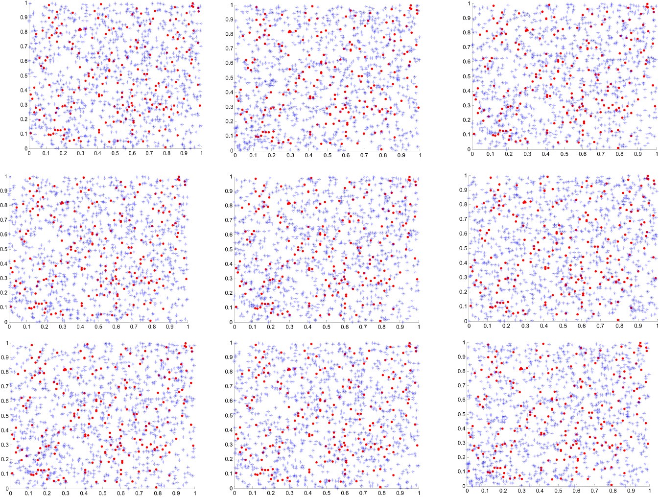
Scatter plots of the transformed observed values (·) versus simulated samples (∗) variables from subfamilies of the copula model. USA (r1 c1), India (r1 c2), UK (r1 c3), Iran (r2 c1), Bolivia (r2 c2), Guatemala (r2 c3), Nigeria (r3 c1), Australia (r3 c2), and South Africa (r3 c3). r: row & c: column.
Finally, we want to investigate the structure of dependency between the number of tests and positivity rate totally. By collecting the data of the 12 countries, 3877 pairs are obtained whose Kendall’s correlation is −0.1434 (P-value: 2.8464 * 10ˆ−19). In addition, we split the data into two parts: peaks and otherwise. This split restricted us to applying marginal distributions – then copulas – because it causes the gap in the number of tests. Table 7 represents the Kendall’s correlations for the countries of interest. It is worth saying that the correlation coefficient for the variables (the number of tests and positivity rate) is negative in both peaks and otherwise.
The correlation between the number of tests and the positivity rate regarding all countries separated based on the peaks.
| Country | Kendall’s tau after removing peaks | P-value | Kendall’s tau for peaks | P-value |
|---|---|---|---|---|
| USA | −0.0168 | 0.8113 | −0.4104 | <0.0001 |
| India | −0.2410 | 0.0001 | 0.0993 | 0.3936 |
| UK | 0.2496 | 0.0015 | −0.7017 | <0.0001 |
| Italy | 0.3309 | <0.0001 | −0.5127 | <0.0001 |
| Iran | 0.0779 | 0.2354 | 0.1574 | 0.1898 |
| UAE | 0.0387 | 0.5348 | −0.1621 | 0.2081 |
| Bolivia | 0.3028 | <0.0001 | −0.2402 | 0.0119 |
| Guatemala | −0.2946 | <0.0001 | – | – |
| Nigeria | 0.4474 | <0.0001 | −0.4197 | <0.0001 |
| Australia | −0.2337 | 0.0003 | −0.6295 | <0.0001 |
| South Korea | 0.3134 | <0.0001 | −0.7214 | <0.0001 |
| South Africa | 0.1203 | 0.0744 | −0.4517 | <0.0001 |
| Total | −0.1381 | <0.0001 | −0.2132 | <0.0001 |
-
Light or dark bolded figures indicate that the coefficient correlation is significantly positive or negative, respectively.
5 Discussion
Generally, at the beginning of an epidemic, the number of tests is low and the proportion of positivity is high. As time passes, the number of tests rises. Also, as the number of new tests increases, the positivity rate falls. The correlation in countries with high number of tests, higher quality of data, is negative and it is commonly between −0.2 and −0.3. By considering all the data as a set, the Kendall’s coefficients are −0.1434, −0.2132, and −0.1381 for total, peaks, and total after removing peaks, respectively. The positivity rate of the tests is significantly better than the frequency of tests to indicate the peaks of the pandemic. The positivity rate is more associated with the number of cases than the number of tests (90% vs 45%).
The proportion of positivity is more proportional than the number of tests to the number of infected cases. Approaching zero positivity rate is a good criterion to scale the success of a healthcare system in fighting against an epidemic. The number and accuracy of tests can play a vital role in the quality level of epidemic data. The policymakers can consider the factors affecting the positivity rate such as the testing policy, restricted facilities, peaks, fluctuations, and so on, and make decisions to prevent misleading because of them. Considering these factors altogether and inputting them in the models like (Khajanchi et al. 2022, 2021; Mondal and Khajanchi 2022) is the correct way to assess function of any intervention of interest.
The first limitation is the low quality of data for some countries because of the restricted facilities, the low number of tests, and non-organized data collection program. Also, some interpolation and moving average methods were applied to find some missing data regarding the countries of interest and calculating the correlation for the countries with poor data. Out of the 12 countries, Iran, South Africa, Nigeria, Bolivia, and Guatemala have got a relatively restricted number of tests. The data of Italy, the UAE, and South Korea showed no significant correlation. The highest quality and most significant correlations belong to the USA, India, the UK, and Australia.
The present approach using copulas is promising since it allows to take into account a wide range of correlation, frequently observed in medical studies. In fact, the classical multivariate models cannot reproduce all type of correlations. Moreover, the standard models are limited, especially because the choice of the marginal distributions is restricted. The crucial step in the modeling process is the choice of the copula function, which best fits the data. Further work is needed to choose the best copulas able to reproduce the dependence structure of bivariate medical variables. In clinical trials or medical studies, sample size is often an important consideration and is relatively small. The copula-based methodology overcomes this limitation as well, because the algorithm can be used to replicate data for any number of patients. The suggested copula-based methodology presented in this paper is simple and easy to implement.
-
Research Funding: None to report.
-
Author contribution: BJ: Idea, Literature, Data, Methods, Programming, Interpretation, First draft. HB: Literature, Methods, Interpretation, Revision. SJZ: Data, Literature, Programming. MR: Design, Final manuscript.
-
Declaration of Interest Statement: We have no conflict of interest to declare.
References
Boubaker, H., and N. Sghaier. 2013. “Portfolio Optimization in the Presence of Dependent Financial Returns with Long Memory: A Copula Based Approach.” Journal of Banking & Finance 37 (2): 361–77, https://doi.org/10.1016/j.jbankfin.2012.09.006.Search in Google Scholar
Bekrizadeh, H., G. A. Parham, and M. R. Zadkarmi. 2013. “Weighted Clayton Copulas and Their Characterizations: Application to Probable Modeling of the Hydrology Data.” Journal of Data Science 11: 293–303, https://doi.org/10.6339/jds.2013.11(2).1084.Search in Google Scholar
Bekrizadeh, H., and B. Jamshidi. 2017. “A New Class of Bivariate Copulas: Dependence Measures and Properties.” Metron 75: 31–50, https://doi.org/10.1007/s40300-017-0107-1.Search in Google Scholar
Bekrizadeh, H., G. A. Parham, and M. R. Zadkarmi. 2017. “A New Asymmetric Class of Bivariate Copulas for Modeling Dependence.” Communications in Statistics – Simulation and Computation 46 (7): 5594–609, https://doi.org/10.1080/03610918.2016.1169292.Search in Google Scholar
Bekrizadeh, H. 2021. “Generalized Family of Copulas: Definition and Properties.” Thailand Statistician 19 (1): 163–78.10.1080/03610918.2022.2032156Search in Google Scholar
Coronavirus (COVID-19) Infection Survey, UK: 8 January 2021. Also available at https://www.ons.gov.uk/peoplepopulationandcommunity/healthandsocialcare/conditionsanddiseases/bulletins/coronaviruscovid19infectionsurveypilot/8january2021.Search in Google Scholar
Corbella, S., and D. D. Stretch. 2013. “Simulating a Multivariate Sea Storm Using Archimedean Copulas.” Coastal Engineering 76: 68–78. https://doi.org/10.1016/j.coastaleng.2013.01.011.Search in Google Scholar
Chatrabgoun, O., Hosseinian-far, and A. Daneshkhah. 2020. “Constructing Gene Regulatory Networks from Microarray Data Using Non-gaussian Pair-Copula Graphical Models.” Journal of Bioinformatics and Computational Biology 47 (59): 1–19.10.1142/S0219720020500237Search in Google Scholar
Clayton, D. G. 1978. “A Model for Association in Bivariate Life Tables and its Application in Epidemiological Studies of Familial Tendency in Chronic Disease Incidence.” Biometrika 65 (1): 141–51. https://doi.org/10.1093/biomet/65.1.141.Search in Google Scholar
Dowdy, D., and G. D’souza. 2020. Covid-19 Testing: Understanding the “Percent Positive”. August 10. Also available at https://www.jhsph.edu/covid-19/articles/covid-19-testing-understanding-the-percent-positive.html.Search in Google Scholar
Embrechts, P., F. Lindskog, and A. McNeil. 2001. Modelling Dependence with Copulas and Applications to Risk Management. ETH Zurich: Department of Mathematics.Search in Google Scholar
Farlie, D. G. J. 1960. “The Performance of Some Correlation Coefficients for a General Bivariate Distribution.” Biometrika 47: 307–23. https://doi.org/10.2307/2333302.Search in Google Scholar
Genest, C. 1987. “Frank’s Family of Bivariate Distributions.” Biometrika 74: 549–55. https://doi.org/10.1093/biomet/74.3.549.Search in Google Scholar
Gumbel, E. J. 1960. “Bivariate Exponential Distributions.” Journal of the American Statistical Association 55: 698–707. https://doi.org/10.1080/01621459.1960.10483368.Search in Google Scholar
Hasell, J., E. Mathieu, D. Beltekian, B. Macdonald, C. Giattino, E. Ortiz-Ospina, M. Roser, and H. Ritchie. 2020. “A Cross-Country Database of COVID-19 Testing.” Scientific Data 7: 345. https://doi.org/10.1038/s41597-020-00688-8. https://ourworldindata.org/coronavirus-testing.Search in Google Scholar
Jamshidi, B., M. Rezaei, S. J. Zargaran, and F. Najafi. 2020. “Mathematical Modeling the Epicenters of Coronavirus Disease-2019 (COVID-19) Pandemic.” Epidemiologic Methods 9 (s1): 20200009. https://doi.org/10.1515/em-2020-0009.Search in Google Scholar
Jamshidi, B., H. Bekrizadeh, S. J. Zargaran, M. Rezaei, and F. Najafi. 2021. “Comparing Length of Hospital Stay during COVID-19 Pandemic in the USA, Italy, and Germany.” International Journal for Quality in Health Care 33 (1): 1–11.10.1093/intqhc/mzab050Search in Google Scholar
Johnson, M. E. 1987. Multivariate Statistical Simulation. Hoboken: John Wiley.10.1002/9781118150740Search in Google Scholar
Kendall, M. G. 1970. Rank Correlation Methods. London: Griffin.Search in Google Scholar
Khajanchi, S., K. Sarkar, and S. Banerjee. 2022. “Modeling the Dynamics of COVID-19 Pandemic with Implementation of Intervention Strategies.” European Physics Journal Plus 137: 129. https://doi.org/10.1140/epjp/s13360-022-02347-w.Search in Google Scholar
Khajanchi, S., K. Sarkar, J. Mondal, K. S. Nisar, and S. F. Abdelwahab. 2021. “Mathematical Modeling of the COVID-19 Pandemic with Intervention Strategies.” Results in Physics 25: 104285. https://doi.org/10.1016/j.rinp.2021.104285.Search in Google Scholar
Li, X., and R. Fang. 2012. “A New Family of Bivariate Copulas Generated by Univariate Distributions.” Journal of Data Science 10: 1–17. https://doi.org/10.6339/jds.201201_10(1).0001.Search in Google Scholar
Morgenstern, D. 1956. “Einfache Beispiele Zweidimensionaler Verteilungen.” Mitteilungsblatt fürMathematische Statistik 8: 234–5.Search in Google Scholar
Mondal, J., and S. Khajanchi. 2022. “Mathematical Modeling and Optimal Intervention Strategies of the COVID-19 Outbreak.” Nonlinear Dynamics 109 (1): 177–202. https://doi.org/10.1007/s11071-022-07235-7.Search in Google Scholar
Nelson, R. 2006. An Introduction to Copulas. New York: Springer-Verlag.Search in Google Scholar
Pearson, K. 1895. “Notes on regression and inheritance in the case of two parents.” Proceedings of the Royal Society of London 58: 240–2.10.1098/rspl.1895.0041Search in Google Scholar
Priest, C. 2003. Correlations: What They Mean and More Importantly What They Don’t Mean. Sydney: The Institute of Actuaries of Australia Biennial Convention.Search in Google Scholar
Roman, M., F. Louzada, V. G. Cancho, and J. G. Leite. 2012. “A New Long-Term Survival Distribution for Cancer Data [Internet].” Journal of Data Science 10 (2): 241–58. http://www.jds-online.com/volume-10-number-2-april-2012.10.6339/JDS.201204_10(2).0005Search in Google Scholar
Sklar, A. 1959. Fonctions de répartition à n dimensions et leurs marges, Vol. 8, 229–31. Paris: Publications de L’Institute Statistical University Paris.Search in Google Scholar
Spearman, C. 1904. “The Proof and Measurement of Association between Two Things.” American Journal of Psychology 15 (1): 72–101. https://doi.org/10.2307/1412159.Search in Google Scholar
Schweizer, B., and E. F. Wolff. 1981. “On Nonparametric Measures of Dependence for Random Variables.” Annals of Statistics 9: 879–85. https://doi.org/10.1214/aos/1176345528.Search in Google Scholar
Wang, G. J., C. Xie, P. Zhang, F. Han, and S. Chen. 2014. “Dynamics of Foreign Exchange Networks: A Time-Varying Copula Approach,” Discrete Dynamics in Nature and Society. Article ID 170921, 11 p. https://doi.org/10.1155/2014/170921.Search in Google Scholar
Wienke, A. 2011. Frailty Models in Survival Analysis. New York: Chapman & Hall/CRC biostatistics series.Search in Google Scholar
Worldometer Website. Also available at https://www.worldometers.info/coronavirus/#countriesSearch in Google Scholar
Zhang, L., and V. P. Singh. 2007. “Bivariate Rainfall Frequency Distributions Using Archimedean Copulas.” Journal of Hydrology 332: 93–109. https://doi.org/10.1016/j.jhydrol.2006.06.033.Search in Google Scholar
© 2023 the author(s), published by De Gruyter, Berlin/Boston
This work is licensed under the Creative Commons Attribution 4.0 International License.
Articles in the same Issue
- Frontmatter
- Articles
- Investigating the Economic Consequence of Terrorism in Sub-Saharan Africa: Evidence from a Dynamic Panel Model
- Model-Based Small Area Estimation of Regional-Level Maternal Mortality Prevalence in Ghana
- NATO’s Expansion and Russia’s Aggressiveness: An Empirical Study from the Perspective of the U.S. Public
- Analysis of the Number of Tests, the Positivity Rate and Their Dependency Structure During COVID-19 Pandemic
- Evaluating Different Covariate Balancing Methods: A Monte Carlo Simulation