Monetary Policy and the Top 10%: A Time-Series Analysis Using ARDL and ECM
-
Nadeen Omar

 and
Christian Richter
and
Christian Richter

Abstract
For the past decades, income inequality has been on the rise, and so is the frequency of its mentions in recent speeches by central bankers. With the heightened importance of the topic, this research aims to study the impact of monetary policy on income inequality. The study used dynamic models for the analysis, namely; the Error-correction Model (ECM) and the Auto-regressive Distributed Lag (ARDL) model to determine the relationship in both the short- and long-run. The data used were the top 10% income share and the short-term interest rate. Our main hypothesis is that changes in the short-term interest rate have a significant impact on the top 10% income share. We draw time-series evidence from a sample of nine economies at different stages of development: United States, United Kingdom, Russia, Germany, France, Greece, China, South Africa and Chile. The findings support the hypothesis with interestingly varying effects across our sample. These results provide important implications that can contribute in bettering policy setting and add to the discussion of the role of central banks in reducing income inequality.
Appendix
A Review of empirical studies on monetary policy and income inequality.
| Study | Country | Period | Method | Monetary policy change | Impact on inequality | |
|---|---|---|---|---|---|---|
| Contractionary monetary policy increases income inequality | ||||||
| Coibion et al. (2017) | US | 1980–2008 | Local projections | Contractionary | Increases inequality | |
| Guerello (2017) | Euro area | 2001–2015 | VAR | Expansionary and QE | Decreases inequality | |
| Mumtaz and Theophilopoulou (2017) | U.K. | 1969–2012 | Structural VAR | Contractionary | Increases inequality | |
| Furceri, Loungani, and Zdzienicka (2018) | Thirty two advanced and emerging economies | 1990–2013 | IRF from local projections | Contractionary | Increases inequality | |
| Casiraghi et al. (2018) | Italy | 2011–2013 | Micro-simulation | QE/UMP | Decreases inequality | |
| Lenza and Slacalek (2018) | France, Germany, Italy, and Spain | 1999Q1–2016Q4 | BVAR and micro-simulation | QE/UMP | Decreases inequality | |
| Contractionary monetary policy decreases income inequality | ||||||
| Saiki and Frost (2014) | Japan | 2008Q4–2013Q3 | VAR | UMP | Increases inequality | |
| Villarreal (2014) | Mexico | 2003–2012 | Local projections | Contractionary | Decreases inequality | |
| O’Farrell, Rawdanowicz, and Inaba (2017) | Eight OECD countries | 2007–2012 | Micro-simulation | Expansionary | Decrease in U.S., Canada, and The Netherlands. Increase in European economies. |
|
| Davtyan (2017) | US | 1983–2012 | VECM | Contractionary | Decreases inequality | |
| Inui, Sudou, and Yamada (2017) | Japan | 1981–2008 | Local projections | Expansionary | Increases inequality | |
| El Herradi and Leroy (2019) | Twelve advanced economies | 1920–2015 | Panel VAR and a single-equation model with local projections | Expansionary | Increases inequality | |
| Cloyne, Ferreira, and Surico (2020) | U.S. and U.K. | U.S.: 1981–2007 U.K.: 1975–2007 | Romer and Romer (2004) procedure | Expansionary | Increases inequality | |
| Dolado, Motyovszki, and Pappa (2021) | U.S. | 1979M1–2016M6 | NK-SAM frictions | Expansionary | Increases inequality | |
Data sample (maximum no. of years obtained).
| Country | Short-term interest rate | Top 10% income share |
|---|---|---|
| United States | 1971Q1–2014Q1 | 1971Q1–2014Q1 |
| United Kingdom | 1986Q1–2016Q1 | 1986Q1–2016Q1 |
| Germany | 1980Q1–2016Q1 | 1980Q1–2016Q1 |
| France | 1980Q1–2016Q1 | 1980Q1–2014Q1 |
| Russia | 1997Q1–2015Q1 | 1997Q1–2015Q1 |
| China | 1997Q3–2015Q1 | 2000Q1–2015Q1 |
| Greece | 1994Q2–2016Q1 | 1994Q2–2016Q1 |
| Chile | 2004Q1–2015Q1 | 2004Q1–2015Q1 |
| South Africa | 1990Q1–2017Q1 | 1990Q1–2017Q1 |
ECM results.
| Country | United States | United Kingdom | France | Russia | South Africa |
|---|---|---|---|---|---|
| Sample (adjusted for lags) |
1983Q2–2014Q1 (124 obs.) |
1988Q4–2016Q1 (110 obs.) |
1980Q2–2014Q1 (136 obs.) |
1999Q4–2015Q1 (62 obs.) |
1998Q2–2017Q1 (76 obs.) |
|
Dependent variable
|
∆ TOP10
t
|
∆ TOP10
t
|
∆ TOP10
t
|
∆ TOP10
t
|
∆ TOP10
t
|
| C | 0.003484 (0.000626) | – | – | – | – |
| ∆ TOP10t−1 | 3.069507 (0.027505) | 2.850251 (0.077547) | 2.687615 (0.048233) | 2.216673 (0.044591) | 2.607693 (0.100118) |
| ∆ TOP10t − 2 | −3.507040 (0.066480) | −3.091203 (0.169356) | −2.758519 (0.095373) | −1.679066 (0.101785) | −2.683514 (0.196039) |
| ∆ TOP10t − 3 | 1.780913 (0.073060) | 1.343358 (0.125373) | 1.185464 (0.093372) | 0.315829 (0.108222) | 1.273684 (0.144435) |
| ∆ TOP10t − 4 | −1.416347 (0.066476) | −1.027340 (0.086095) | −0.844045 (0.110127) | −0.924713 (0.109331) | −1.046205 (0.144255) |
| ∆ TOP10t − 5 | 3.167672 (0.077325) | 2.731838 (0.188359) | 1.971114 (0.159059) | 2.264273 (0.129471) | 2.272839 (0.360903) |
| ∆ TOP10t − 6 | −3.553632 (0.086904) | −2.996910 (0.219878) | −2.025221 (0.156287) | −1.521462 (0.080852) | −2.321162 (0.368091) |
| ∆ TOP10t − 7 | 1.744711 (0.066798) | 1.206523 (0.117157) | 0.779942 (0.065758) | – | 0.936600 (0.146428) |
| ∆ TOP10t − 8 | −0.314812 (0.024782) | – | – | – | – |
| ∆ TOP10t − 9 | – | – | – | 0.561536 (0.040360) | – |
| ∆ TOP10t−10 | – | −0.077403 (0.019266) | −0.030570 (0.009727) | −0.342708 (0.031460) | −0.052637 (0.015793) |
| ∆ INTQt | – | −0.006064 (0.002488) | −0.001521 (0.000546) | −0.003683 (0.001055) | −0.005516 (0.002427) |
| ∆ INTQt−1 | – | – | – | – | – |
| ∆ INTQt − 2 | – | – | – | – | – |
| ∆ INTQt − 3 | – | – | – | – | – |
| ∆ INTQt − 4 | 0.004123es (0.001333) | 0.005475 (0.002181) | – | – | – |
| ∆ INTQt − 5 | – | – | −0.003070 (0.000980) | – | – |
| ∆ INTQt − 6 | – | – | – | – | – |
| ∆ INTQt − 7 | – | – | – | – | – |
| ∆ INTQt − 8 | – | – | – | – | – |
| ∆ INTQt − 9 | – | – | – | – | – |
| ∆ INTQt−10 | – | – | – | – | – |
| ECTt−1 | −0.001209 (0.000378) | −0.006665 (0.003142) | −0.005405 (0.001560) | −0.010685 (0.002640) | −0.020039 (0.005204) |
| Dummy (structural break) | – | 0.099635 (0.010137) | – | – | – |
| Dummy (positive outliers) | 0.045437 (0.002122) | – | 0.032248 (0.006218) | 0.068294 (0.004460) | – |
| Dummy (negative outliers) | −0.036881 (0.003007) | – | −0.024497 (0.004016) | −0.069292 (0.010583) | – |
| R 2 | 0.999428 | 0.996525 | 0.997652 | 0.998346 | 0.995790 |
| Adjusted R 2 | 0.999366 | 0.996134 | 0.997423 | 0.997982 | 0.995216 |
| DW statistic | 1.717920 | 1.932719 | 1.722462 | 1.775729 | 2.038342 |
| S.E. of regression | 0.004759 | 0.019425 | 0.007491 | 0.021650 | 0.021622 |
| LR coefficient | −0.972296 | −0.298378 | −0.282019 | −0.153883 | −0.271646 |
-
*All variables included are statistically significant at 5% and all models were checked for autocorrelation and heteroscedasticity; es, exponential smoothing; – = does not apply; () includes standard error of the coefficients.
ARDL results.
| Country | Germany | Chile | China | Greece | ||
|---|---|---|---|---|---|---|
| Sample (adjusted for lags) | 1982Q4–2016Q1 (134 obs.) | 2006Q1–2013Q4 (32 obs.) | 2001Q1–2015Q1 (57 obs.) | 1996Q4–2016Q1 (78 obs.) | ||
| Dependent variable | ∆ TOP10t | TOP10t | TOP10t | TOP10t | ||
| C | 0.073485 (0.013304) | 2.788105 (0.718769) | 0.477802 (0.176245) | 0.110691 (0.035428) | ||
| ∆ TOP10t − 1 | TOP10t − 1 | 2.854849 (0.045755) | −0.002075 (0.000385) | 3.311579 (0.106029) | 3.184963 (0.099578) | 3.834818 (0.095365) |
| TOP10t − 2 | −3.278517d (0.118984) | −4.588927 (0.296774) | −4.161875 (0.266475) | −5.945079 (0.290375) | ||
| TOP10t − 3 | 1.854910d (0.148515) | 3.244637 (0.318631) | 2.774067 (0.267643) | 4.609347 (0.351702) | ||
| TOP10t − 4 | −1.370045d (0.132456) | −1.969754 (0.262054) | −1.810678 (0.243627) | −2.588678 (0.216820) | ||
| TOP10t − 5 | 2.430210d (0.183737) | 2.923204 (0.678437) | 2.949491 (0.491562) | 3.552954 (0.334263) | ||
| TOP10t − 6 | −2.473322d (0.171131) | −3.841791 (0.812115) | −3.648765 (0.556677) | −5.197256 (0.541891) | ||
| TOP10t − 7 | 1.012991d (0.072736) | 2.578326 (0.496640) | 2.284748 (0.337455) | 3.975559 (0.441095) | ||
| TOP10t − 8 | – | −0.709429 (0.132110) | −0.583060 (0.090101) | −1.320391 (0.166938) | ||
| TOP10t − 9 | – | – | – | – | ||
| TOP10t − 10 | −0.070621d (0.008695) | – | – | 0.075064 (0.016402) | ||
| INTQt | – | – | −0.028260es (0.006763) | – | ||
| INTQt − 1 | – | – | 0.027289es (0.008891) | – | ||
| INTQt − 2 | – | – | – | – | ||
| INTQt − 3 | −0.001538 (0.000316) | – | – | – | ||
| INTQt − 4 | – | – | −0.036627es (0.015661) | – | ||
| INTQt − 5 | – | – | 0.041975es (0.018506) | – | ||
| INTQt − 6 | – | – | – | – | ||
| INTQt − 7 | – | 0.009236 (0.002968) | – | 0.003854 (0.001735) | ||
| INTQt − 8 | – | – | – | 0.004111 (0.001656) | ||
| INTQt − 9 | – | – | −0.039254es (0.014066) | – | ||
| INTQt − 10 | – | – | 0.032643es (0.011380) | – | ||
| Dummy (structural break) | – | – | – | – | ||
| Dummy (positive outliers) | 0.028010 (0.003339) | – | – | – | ||
| Dummy (negative outliers) | −0.015255 (0.002494) | – | – | – | ||
| R 2 | 0.998605 | 0.999010 | 0.999934 | 0.999923 | ||
| Adjusted R 2 | 0.998467 | 0.998605 | 0.999912 | 0.999911 | ||
| DW statistic | 1.901167 | 2.255174 | 2.077281 | 2.089316 | ||
| S.E. of regression | 0.007113 | 0.036217 | 0.013092 | 0.016293 | ||
| Steady state | −0.7412048 | 0.179557 | −0.201098 | 0.07018 | ||
-
*All variables included are statistically significant at 5% and all models were checked for autocorrelation and heteroscedasticity; d, differenced dependent variable lag; es, exponential smoothing; – = does not apply; () includes the standard error of the coefficients.
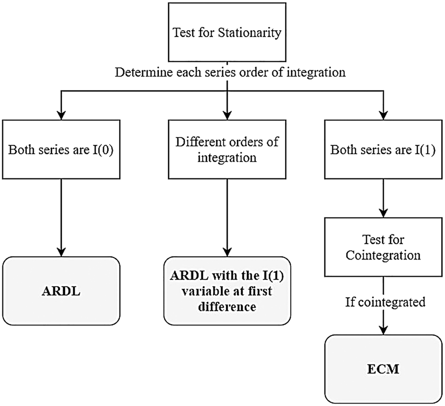
Methodological approach.
References
Ajani, H. A. 1978. “Quarterly Interpolation of Constant Price Gross Domestic Product of Nigeria-1963/64-1972/73.” Economic and Financial Review 16 (2): 2.Search in Google Scholar
Ajao, I. O., A. G. Ibraheem, and F. J. Ayoola. 2012. “Cubic Spline Interpolation: A Robust Method of Disaggregating Annual Data to Quarterly Series.” Journal of Physical Sciences and Environmental Safety 2 (1): 1–8.Search in Google Scholar
Bernanke, B. S. 2015. Monetary Policy and Inequality. Economic Commentary (Federal Reserve Bank of Cleveland). Also available at https://www.brookings.edu/blog/ben-bernanke/2015/06/01/monetary-policy-and-inequality/.Search in Google Scholar
Casiraghi, M., E. Gaiotti, L. Rodano, and A. Secchi. 2018. “A “Reverse Robin Hood”? The Distributional Implications of Non-Standard Monetary Policy for Italian Households.” Journal of International Money and Finance 85: 215–35, https://doi.org/10.1016/j.jimonfin.2017.11.006.Search in Google Scholar
Cloyne, J., C. Ferreira, and P. Surico. 2020. “Monetary Policy when Households Have Debt: New Evidence on the Transmission Mechanism.” The Review of Economic Studies 87 (1): 102–29, https://doi.org/10.1093/restud/rdy074.Search in Google Scholar
Coibion, O., Y. Gorodnichenko, L. Kueng, and J. Silvia. 2017. “Innocent Bystanders? Monetary Policy and Inequality.” Journal of Monetary Economics 88: 70–89, https://doi.org/10.1016/j.jmoneco.2017.05.005.Search in Google Scholar
Davtyan, K. 2017. “The Distributive Effect of Monetary Policy: The Top One Percent Makes the Difference.” Economic Modelling 65: 106–18, https://doi.org/10.1016/j.econmod.2017.05.011.Search in Google Scholar
Dolado, J. J., G. Motyovszki, and E. Pappa. 2021. “Monetary Policy and Inequality Under Labor Market Frictions and Capital-Skill Complementarity.” American Economic Journal: Macroeconomics 13 (2): 292–332, https://doi.org/10.1257/mac.20180242.Search in Google Scholar
El Herradi, M., and A. Leroy. 2019. “Monetary Policy and the Top One Percent: Evidence from a Century of Modern Economic History.” De Nederlandsche Bank Working Paper (Issue 632), 1–40, https://doi.org/10.2139/ssrn.3379740.Search in Google Scholar
Furceri, D., P. Loungani, and A. Zdzienicka. 2018. “The Effects of Monetary Policy Shocks on Inequality.” Journal of International Money and Finance 85: 168–86, https://doi.org/10.1016/j.jimonfin.2017.11.004.Search in Google Scholar
Galli, R., and R. Van der Hoeven. 2001. Is Inflation Bad for Income Inequality: The Importance of the Initial Rate of Inflation. ILO Employment Paper. No. 2001/29. Search in Google Scholar
Guerello, C. 2017. “Conventional and Unconventional Monetary Policy vs. Households Income Distribution: An Empirical Analysis for the Euro Area.” Journal of International Money and Finance 85: 187–214, https://doi.org/10.1016/j.jimonfin.2017.11.005.Search in Google Scholar
Inui, M., N. Sudo, and T. Yamada. 2017. “The Effects of Monetary Policy Shocks on Inequality in Japan.” Bank of Japan Working Paper 17-E-3, Bank of Japan, Tokyo.Search in Google Scholar
Lenza, M., and J. Slacalek. 2018. “How Does Monetary Policy Affect Income and Wealth Inequality? Evidence from Quantitative Easing in the Euro Area.” In ECB Working Paper Series (Issue 2190). Frankfurt a. M.: European Central Bank (ECB), http://dx.doi.org/10.2866/414435.10.2139/ssrn.3275976Search in Google Scholar
Monnin, P. 2017. “Monetary Policy, Macroprudential Regulation and Inequality.” Council on Economic Policies Discussion Note, 12 April 2017, https://doi.org/10.2139/ssrn.2970459.Search in Google Scholar
Mumtaz, H., and A. Theophilopoulou. 2017. “The Impact of Monetary Policy on Inequality in the UK. An Empirical Analysis.” European Economic Review 98: 410–23, https://doi.org/10.1016/j.euroecorev.2017.07.008.Search in Google Scholar
O’Farrell, R., and L. Rawdanowicz. 2017. “Monetary Policy and Inequality: Financial Channels.” International Finance 20 (2): 174–88, https://doi.org/10.1111/infi.12108.Search in Google Scholar
Romer, C. D., and D. H. Romer. 1989. “Does Monetary Policy Matter? A New Test in the Spirit of Friedman and Schwartz.” NBER Macroeconomics Annual 4: 121–70, https://doi.org/10.1086/654103.Search in Google Scholar
Romer, C. D., and D. H. Romer. 2004. “A New Measure of Monetary Shocks: Derivation and Implications.” American Economic Review 94 (4): 1055–84, doi:https://doi.org/10.1257/0002828042002651.Search in Google Scholar
Saiki, A., and J. Frost. 2014. “Does Unconventional Monetary Policy Affect Inequality? Evidence from Japan.” Applied Economics 46 (36): 4445–54, https://doi.org/10.1080/00036846.2014.962229.Search in Google Scholar
Villarreal, F. G. 2014. Monetary Policy and Inequality in Mexico. MPRA Paper 57074. Online at http://mpra.ub.uni-muenchen.de/57074/.Search in Google Scholar
© 2021 Walter de Gruyter GmbH, Berlin/Boston
Articles in the same Issue
- Frontmatter
- Editors Note
- Editor’s Note
- Special on COVID-19 Research
- Covid-19 Response Models and Divergences Within the EU: A Health Dis-Union
- Landscape Political Ecology: Rural-Urban Pattern of COVID-19 in Nigeria
- The Relationship Between Poverty and COVID-19 Infection and Case-Fatality Rates in Germany during the First Wave of the Pandemic
- Covid-19: A Trade-off between Political Economy and Ethics
- Special on Inequality, Policy and Society
- Causes and Consequences of Income Inequality – An Overview
- Monetary Policy and the Top 10%: A Time-Series Analysis Using ARDL and ECM
- Trade Intensity, Fiscal Integration and Income Inequality in ECOWAS
- Empirical Analysis of the Effect of Fiscal Policy Shocks in China
- The Political Economy of Sectoral Credit Provisioning in India: An Empirical Analysis
- Perspectives on Gender Stereotypes: How Did Gender-Based Perceptions Put Hillary Clinton at an Electoral Disadvantage in the 2016 Election?