Block diagonalization of (p, q)-tridiagonal matrices

Hariprasad Manjunath

doi:10.1515/spma-2025-0041

Article Open Access

Block diagonalization of (p, q)-tridiagonal matrices

Hariprasad Manjunath

Published/Copyright: August 21, 2025

Published by

Become an author with De Gruyter Brill

Submit Manuscript Author Information Explore this Subject

From the journal Special Matrices Volume 13 Issue 1

Abstract

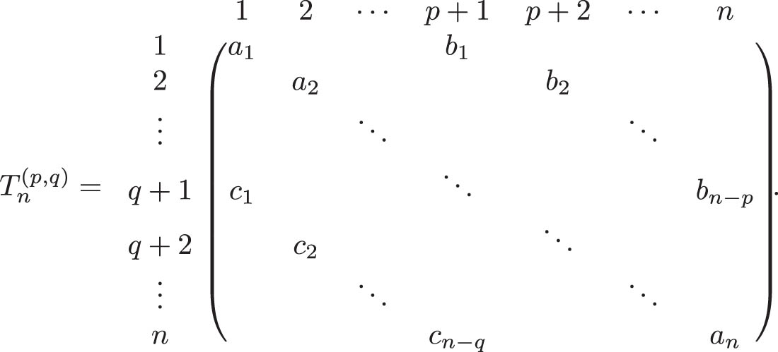
In this article, we study the block diagonalization of ( p , q ) -tridiagonal matrices and derive closed-form expressions for the number and structure of diagonal blocks as functions of the parameters p , q , and n . This reduction enables efficient computation of eigenvalues and eigenvectors by decomposing the matrix into smaller subproblems. We extend the method to more general ( P , Q ) -tridiagonal matrices, where P and Q are sets of positive integers, covering general banded structures. We also examine special cases such as bidiagonal and triangular block reductions along with supporting algorithms and numerical examples.

Keywords: k-tridiagonal matrices; p, q-tridiagonal matrices; upper Hessenberg; eigenvalues

MSC 2010: 15A18; 65F15; 47B36

1 Introduction

An n × n matrix is a ( p , q ) -tridiagonal matrix if it is of the form (1)

When p = q = 1 , the matrix is tridiagonal. When p = q = k , they are known as k -tridiagonal matrices. The inverses of k tridiagonal matrices are studied in [14]. In [18] and [14], explicit construction of permutation matrices was given fork diagonalization of k -tridiagonal matrices. da Fonseca et al. [4] explained the historical connection with trigonometric polynomials and the development of algorithms for k -tridiagonal matrices and ( p , q ) -pentadiagonal matrices. da Fonseca et al. [4] also mentioned the graph-theoretic approach, which we follow in this study. da Fonseca and Yılmaz [6] derived the determinant spectra and inversion of k -tridiagonal matrices.

As an extension of k -tridiagonal matrices, when p = k , q = k + 1 , the ( k , k + 1 ) -tridiagonal matrices are studied in [19]. Takahira et al. [19] derived the bidiagonalization using a permutation matrix. The ( k , k + 1 ) tridiagonal matrices arise in discrete hungry Lotka-Volterra models [10]. In particular, when ⌈ n 2 ⌉ ≤ p < q , a bidiagonal reduction of T n ( p , q ) is possible by a permutation matrix. Recently, a bidiagonalization reduction of ( p , q ) -tridiagonal matrices was investigated in [12]. The bidiagonalization was further used to compute the inverse of these matrices. The bidiagonalization of the blocks for the k -tridiagonal block matrices is studied in [13]. In general, we do not have the bidiagonal reduction of ( p , q ) -tridiagonal matrices. The determinants and their properties are studied in [7]. The eigenvalues of double-banded matrices are studied in [16]. These structured tridiagonal matrices are applied in boundary value problems [9], and in the discretization of differential equations [1]. They are also of interest in number theory [5].

2 Notations

The greatest common divisor of two integers a , b is denoted by GCD ( a , b ) . The identity matrix of order n is denoted by I n (or I in the absence of ambiguity). The adjacency matrix of a directed cycle is denoted by C , which is C = 0 1 I n − 1 0 . Throughout, a path refers to a path in the directed graph defined by the adjacency matrix.

3 Summary of the results

In Table 1, we summarize our results on block diagonal reduction of ( p , q ) -tridiagonal matrices for even n . For odd n , the number of blocks can be deduced from the number of blocks in T n − 1 ( p , q ) using Theorem 9. Table 1 gives the relation between p , q , n and the corresponding number of irreducible blocks in the block diagonalization and the nature of the individual blocks. The different support graphs of the individual blocks lead to the nine distinct cases outlined in Table 1.

Table 1

Number of blocks in the block diagonal reduction of T n ( p , q ) and nature of the blocks for even n (for odd n , the number of blocks can be deduced by Theorem 9)

Condition on p and q	Number of blocks	Nature of blocks
p + q ≤ n , d = GCD ( p , q )	d	Each block is ( p ′ , q ′ ) -tridiagonal with p ′ = p d , q ′ = q d
p = n 2 , q > p	q − p	n − q paths with four vertices each
2 q > 3 p		2 q − 3 p paths containing two vertices
p = n 2 , q > p	q − p	r paths with ( 2 k + 2 ) vertices each
2 q < 3 p		q − p − r paths containing 2 k vertices
( q − p ) k + r = n 2
p , q > n 2	p + q − n	2 p − n isolated vertices, nature of remaining blocks to be deduced from rows two and three of this table depending on values of p ′ = n − p , q ′ = n + q − 2 p , n ′ = 2 n − 2 p
p + q > n	p	n − q cycles of length 1 + q p
p < n 2		p + q − n paths of length q p
p ∣ q
p + q > n	p + q − n	p − r paths have t vertices
p < n 2		r − 2 ( n − q ) paths have t + 1 vertices
r = n mod p , n = p t + r ,		n − q paths have 2 t + 2 vertices
r > 2 ( n − q ) − 1
p + q > n	p + q − n	p − r paths have t vertices
p < n 2		length of remaining paths depends on r , n − q
r = n mod p , n = p t + r ,
( n − q ) < r ≤ 2 ( n − q ) − 1
p + q > n	p + q − n	r − ( n − q − r 2 ) paths with t 2 ( t 1 + 1 ) vertices each
p < n 2		r 2 paths with ( t 1 + 1 ) ( t 2 + 1 ) vertices each
r = n mod p , n = p t 1 + r		( p − r ) paths with t 1 vertices each
r < n − q ,
r > 2 ( n − q ) − p − 1
r = t 2 ( r − ( n − q ) ) + r 2
p + q > n	d if d ≥ p + q − n	d − ( p + q − n ) of them are cycles, while remaining are paths
p < n 2	p + q − n if d < p + q − n
r = n mod p , n = p t + r
r < n − q , r ≤ 2 ( n − q ) − p − 1
d = GCD ( p , q )

We present an algorithm for the bidiagonal reduction of T n ( p , q ) when n 2 ≤ p < q . In Section 6, we prove that an upper or lower triangular reduction of T n ( P,Q ) is possible when P = { p 1 < p 2 < … < p k } and Q = { q 1 < q 2 < … < q l } with n 2 ≤ p 1 < … < p k < q 1 < … < q l .

4 Block diagonal reduction of ( p , q ) -tridiagonal matrices and their nature

Let A ( p , q ) denote the matrix with ones along the p th upper diagonal and q th lower diagonal, i.e. A ( i , j ) = 1 if i − j = p or j − i = q . The matrix A ( p , q ) is the support of the non-diagonal entries of T n ( p , q ) . We consider the directed graph represented by the adjacency (incidence) matrix A ( p , q ) . A ( p , q ) ( i , j ) = 1 , if there is an edge from vertex i to vertex j . Let [ n ] = { 1 , 2 , 3 , … , n } .

Starting with a vertex s , from the matrix A ( p , q ) , it has out neighbour v 1 = s + p , v 2 = s − q and in neighbours v 3 = s − p , v 4 = s + q given 1 ≤ v i ≤ n for i = 1 , 2, 3, 4. If any of the neighbour v j ∉ [ n ] it is not a neighbour of s in the graph.

Then, to obtain the connected component corresponding to vertex s , we consider ( i , j ) ∈ Z 2 and r ∈ [ n ] such that

p i + q j + s = r ,

where ( i , j ) is either (0, 0) (the vertex s itself) or ( i , j ) is connected to (0, 0). We say ( i , j ) ∈ Z 2 is connected to (0, 0) if there is a path ℒ of feasible vertices ( 1 ≤ p x + q y + s ≤ n , ∀ ( x , y ) ∈ ℒ ) formed by either moving right or left (vertices ( x ± 1 , y ) ) or moving up or down (vertices ( x , y ± 1 ) ), connecting ( i , j ) to (0, 0).

Let

C s = { r ∣ p i + q j + s = r for ( i , j ) connected to ( 0,0 ) } .

Then, we have the disjoint union

[ n ] = ⨆ s ∈ S C s .

Let the number of equivalent classes be k ( ∣ S ∣ = k ).

Let e r be r th canonical basis vector in R n . Let the columns of the matrices P s be e r ∈ R n for r ∈ C s . We arrange the columns of P s in the lexicographic order of ( i , j ) .

Let P be the permutation matrix such that

(2) P = [ P s 1 P s 2 P s 3 … P s k ] .

Then, we have the following theorem.

Theorem 1

The matrix P T T n ( p , q ) P is block-diagonal with k blocks and each block is of size ∣ C s ∣ for s ∈ S .

Proof

Consider the directed graph corresponding to A ( p , q ) . Then, the set C s defines a connected component that starts with the vertex s . Thus, the similarity transform by P will rearrange the vertices such that the connected components are next to each other. Thus, reducing the matrix into a block diagonal form. Since A ( p , q ) is support of T n p , q on non-diagonal entries, the matrix P also block diagonalizes T n ( p , q ) .□

Consider a situation when a connected component is a directed path. Define the “matrix order” to be the order of the vertices according to the adjacency matrix A ( p , q ) . Let the “latent order” be the order of vertices in such a way that they form a directed path starting from left to right. We intend to find a permutation for converting matrix order to the latent order.

The following Lemma 1 gives a situation when every connected component is a path.

Lemma 1

If p + q ≥ n , then every connected component of A ( p , q ) is either a path or a loop (cycle). Further when n 2 ≤ p < q every connected component is a path.

Proof

Since n − p < q , rows 1 to n − p have a single one each and rows q + 1 to n have single one each. Therefore, in the graph corresponding to A , every vertex has at most one incoming edge. Similarly, columns 1 to n − q have a single one each, and columns p + 1 to n have a single one each. Therefore, every vertex has at most one outgoing edge.

Starting with an arbitrary vertex in a connected component, one can move right (in the direction of the arrow) or left (against the direction of the arrow). If we continue this traversal and the two ends meet, then we obtain a directed cycle. Otherwise, we obtain a directed path.

Let q > p ≥ n 2 , and assume there is a cycle. Then, to move right from an arbitrary position in the latent order, we have r + p , r + p − q , r + 2 p − q , r + 2 p − 2 q , … . If we move left in the latent order, r + q , r + q − p , r + 2 q − p , r + 2 q − 2 p , … The first sequence is of the form r + k ( p − q ) , r + k ( p − q ) + p , the second sequence is of the form r + l ( q − p ) , r + l ( q − p ) + q . If there is a loop, then these two sequences must meet at some point. If

r + k p − ( k − 1 ) q = r + l q − ( l − 1 ) p , ( k + l − 1 ) p = ( k + l − 1 ) q , p = q .

This leads to a contradiction. On the other hand, if r − k ( q − p ) + p = r + l ( q − p ) Then, we obtain p = ( k + l ) ( q − p ) . We also have r + k ( q − p ) ∈ [ n ] since r − k ( q − p ) + p ∈ [ n ] . Therefore, we obtain r ≥ 1 + k ( q − p ) . Similarly, we have r + ( l − 1 ) ( q − p ) + q ≤ n . This implies

1 + ( k + l − 1 ) ( q − p ) + q ≤ n , 1 + p + q ≤ n + ( q − p ) , 1 + 2 p + ( q − p ) ≤ n + ( q − p ) .

Since we know 2 p ≥ n , this also gives a contradiction. Therefore, when n 2 ≤ p < q , we do not obtain a cycle in a connected component.□

Algorithm 1. Obtain connected components
1:	Input : n , p , q , marked vertices M = ϕ
2:	Output: Connected components C s Lexicographic order Q s .
3:	while [ n ] \ M ≠ ϕ do
4:	take s ∈ [ n ] \ M .
5:	C s , Q s i = L D F S ( n , p , q , s )
6:	M = M ∪ C s .

Algorithm 2. Lexicographic depth-first search (LDFS)
1:	n , p , q , s , marked vertices M = ϕ , stack S t
2:	Connected component C s Lexicographic order Q s .
3:	Append ( Q s , ( 0,0 ) )
4:	Append ( M , s ) .
5:	push( N e i g h b o u r s ( s , ( 0,0 ) ) , S t )
6:	while Stack S t is not empty do
7:	v , ( i , j ) = pop(St)
8:	if v ∩ M = ϕ then
9:	Append ( M , v ) , Append ( Q s , ( i , j ) ) .
10:	push( N e i g h b o u r s ( v , ( i , j ) ) , S t )
11:	C s = M .
12:	Sort vertices in C s according to the lexicographic order given in Q s .

Algorithm 3. Neighbour ( v , ( i , j ) )
1:	v , p , q .
2:	N s = ϕ , Q s = ϕ , l 1 , l 2 , r 1 , r 2 .
3:	if v − p > 0 then
4:	l 1 = v − p , d l 1 = ( i − 1 , j ) .
5:	Append ( N s , l 1 )
6:	Append ( Q s , d l 1 )
7:	if v − q > 0 then
8:	l 2 = v − q , d l 2 = ( i , j + 1 ) .
9:	Append ( N s , l 2 )
10:	Append ( Q s , d l 2 )
11:	if v + p ≤ n then
12:	r 1 = v + p , d r 1 = ( i + 1 , j ) .
13:	Append ( N s , r 1 )
14:	Append ( Q s , d r 1 )
15:	if v + q ≤ n then
16:	r 2 = v + q , d r 2 = ( i , j − 1 ) .
17:	Append ( N s , r 2 )
18:	Append ( Q s , d r 2 )
19:	Return N s , Q s

Theorem 2

When the indices ( i , j ) determining the columns of P s are in lexicographic order and the corresponding e r form the columns of P s , we obtain the bidiagonalization when a connected component is a path.

Proof

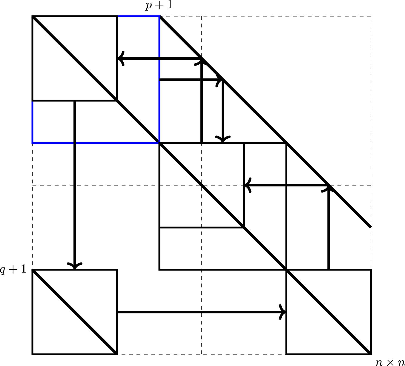
In the lexicographic Depth First Search, starting with an arbitrary vertex r = ( 0,0 ) , we move right in the latent order, in steps of p , it will increase the first coordinate (Figure 1, we move starting from the origin in the positive p axis). If the vertex ( i , 0 ) does not have any vertex to the right in the matrix order, then we move left in the matrix order in steps of q , this will increase the second coordinate (the second axis is − q , in Figure 1, we move from C to D increasing − q ). Then, we reach ( i , j ) , which does not have any vertex to the left in the matrix order, we again move right by increasing p , till we reach a vertex with degree one ( E 1 in Figure 1). Now, the left neighbour of (0, 0) is either ( − 1 , 0 ) or ( 0 , − 1 ) . Thus, we move left by decreasing the first coordinate ( − i , 0 ) and then, decreasing the second coordinate, etc. In conclusion, moving right in the latent order will increase the coordinates in the p , − q plane, and moving left will decrease the coordinates. Thus, the lexicographic order will preserve the path.□

$Figure 1 Depth-first search starting at (0, 0) marks the nodes in the path along the arrow in the upper right quadrant ((0, 0) to E 1 {E}_{1} ) and then again visits the left neighbour and traces the arrow in the lower left quadrant ((0, 0) to E 2 {E}_{2} ). Ordering the nodes lexicographically along the ( p , − q ) \left(p,-q) axis will trace the nodes in the path ( E 2 {E}_{2} to E 1 {E}_{1} ).$

Figure 1

Depth-first search starting at (0, 0) marks the nodes in the path along the arrow in the upper right quadrant ((0, 0) to E 1 ) and then again visits the left neighbour and traces the arrow in the lower left quadrant ((0, 0) to E 2 ). Ordering the nodes lexicographically along the ( p , − q ) axis will trace the nodes in the path ( E 2 to E 1 ).

As a corollary of the above theorem, we have block bidiagonalization when ⌈ n 2 ⌉ ≤ p < q < n .

Corollary 1

When ⌈ n 2 ⌉ ≤ p < q < n , and the permutation matrix P is constructed according to the LDFS, we obtain P T T n ( p , q ) P as a block bidiagonal matrix.

Next we look at the number of diagonal blocks and their nature in the block diagonal reduction of T n ( p , q ) .

Remark

Unless otherwise stated, we assume n is even in the following theorems. For odd n , Theorem 9 relates this to the number of blocks for T n − 1 ( p , q ) .

Theorem 3

If p + q < n , then we have d = GCD ( p , q ) many diagonal blocks.

Proof

Consider equivalence classes C 1 , C 2 , … C d . Now, we need to prove that C s ≠ C t for any i , j ∈ [ d − 1 ] . Suppose C s = C t , then we have for some index r ∈ C s .

s + i p + j q = t + a p + b q s − t = ( a − i ) p + ( b − j ) q .

Now, d divides ( a − i ) p + ( b − j ) q so it should divide s − t . But we have ∣ s − t ∣ < d . So s = t . This proves that there are at least d diagonal blocks.

From any arbitrary vertex, we can trace back to a vertex number r ≤ p via the p th upper diagonal. Then, it is sufficient to prove that every element of [ p ] belongs to one of C s for s < d .

Let p = w d . Without loss of generality, we show that every vertex m d + 1 for m = 0 , 1 , … w is reachable to C 1 . From the Euclid’s algorithm, we have m d = m k 1 p − m k 2 q . With m , k 1 , k 2 ≥ 0 . So m d is represented by ( m k 1 , − m k 2 ) . Now, we can go to the right by the amount q because m d + q ≤ n . Thus, the tuple reduces to ( m k 1 , − ( m k 2 − 1 ) ) . Now, we can continue going to the right by q or going to the left by p depending on the resulting number. Let ( i , − j ) be an intermediate stage, if i , j > 1 , then we can always go right by p or go left by q , otherwise, we obtain p + q > n , which is a contradiction. The procedure ends only at the index (0, 0), which corresponds to vertex 1.□

Remark 1

The above theorem gives a simple procedure to reduce the T n ( p , q ) to block banded matrices when p + q < n and d = GCD ( p , q ) . Starting with the first vertex, consider vertices 1 , d + 1 , 2 d + 1 , 3 d + 1 , … , they form a connected component. Similarly, the vertices r , r + d , r + 2 d , r + 3 d , … form a connected component for 1 ≤ r ≤ d .

From Remark 1, each block diagonal matrix is ( p ′ , q ′ ) -tridiagonal with p ′ = p d and q ′ = q d . Let n ′ = ⌊ n d ⌋ , we have p ′ + q ′ ≤ n ′ . In addition, we have GCD ( p ′ , q ′ ) = 1 , implying that no further block diagonal reduction is possible.

Example 1

Consider A ( 2 , 4 ) = 0 0 0 0 1 0 0 0 0 0 0 0 0 0 0 1 0 0 0 0 1 0 0 0 0 0 1 0 0 0 0 1 0 0 0 0 0 1 0 0 0 0 1 0 0 0 0 0 1 0 0 0 0 1 0 0 0 0 0 1 0 0 0 0 1 0 0 0 0 0 0 0 0 0 0 1 0 0 0 0 0 0 0 0 0 0 1 0 0 0 0 0 0 0 0 0 0 1 0 0 10 × 10 . We have G C D ( 2 , 4 ) = 2 and 2 + 4 < 10 . As per Remark 1, we can have C 1 = { 1 , 3 , 5 , 7 , 9 } and C 2 = { 2 , 4 , 6 , 8 , 10 } . Let e j be the j th canonical basis vector. The permutation matrix P = e 1 e 3 e 5 e 7 e 9 e 2 e 4 e 6 e 8 e 10 will give the block diagonal reduction P T A ( 2 , 4 ) P = T 1 T 2 = 0 0 1 1 0 0 1 1 0 0 1 1 0 0 1 0 0 0 1 1 0 0 1 1 0 0 1 1 0 0 1 0 .

Example 2

For the eigenvalue computation, we consider the block diagonal reduction of T n ( p , q ) with n varying over the set { 2 4 , 2 5 , … , 2 12 } , and corresponding values of p ∈ { 2 , 2 2 , 2 3 , … , 2 10 } and q ∈ { 2 2 , 2 3 , … , 2 11 } . Figure 2(a) demonstrates that the time taken by the block diagonal reduction is significantly lower compared to the unreduced case. This can be understood as follows: if we solve a fixed-size problem of size k exactly n ⁄ k times, and the method used has a complexity of O ( n α ) for some constant α , then the total computational cost becomes O ( ( n ⁄ k ) ⋅ k α ) = O ( n ⋅ k α − 1 ) . Since both k and α are constants, this results in an overall linear complexity in n . In Figure 2(b), n varies as before, but the parameters are fixed at p = 2 and q = 4 . This setup affects only the constant factor in the computational complexity. As a result, the logarithmic plot in Figure 2(b) shows two approximately parallel lines, which is consistent with the expected theoretical complexity.

Figure 2

For n varying as a power of 2, (a) increases p and q respectively in the power of two and (b) keeps p = 2 and q = 2 constant while n is varied in power of two. (a) Varying block size and (b) constant blocksize.

Theorem 4

When p = n 2 , and q > p , then there are q − p blocks.

Proof

Start with the block A ( p , q ) ( p + 1 : q , p + 1 : q ) , and trace back in anticlockwise order in the matrix. Then, we can see that all the blocks are connected. The vertices inside the block are disconnected. Thus, we have q − p connected components. The proof is illustrated in Figure 3.□

$Figure 3 When p = n 2 p=\frac{n}{2} and q > p q\gt p , the connectivity of ( p − q ) × ( p − q ) \left(p-q)\times \left(p-q) block (in blue) with the rest of the diagonal entries, is obtained by tracing in the anticlockwise direction along the arrow. Thus, we obtain p − q p-q connected components. There are n − q n-q paths of length four and q − p − ( n − q ) = 2 q − 3 p q-p-\left(n-q)=2q-3p paths of length two.$

Figure 3

When p = n 2 and q > p , the connectivity of ( p − q ) × ( p − q ) block (in blue) with the rest of the diagonal entries, is obtained by tracing in the anticlockwise direction along the arrow. Thus, we obtain p − q connected components. There are n − q paths of length four and q − p − ( n − q ) = 2 q − 3 p paths of length two.

Theorem 5

If p , q > n 2 , then there are q + p − n blocks.

Proof

The columns n − q + 1 to p have only diagonal entries. The rows in n − p + 1 , to q will have only the diagonal entry. If p < q , then we have the indices n − p + 1 to p corresponding to only diagonal entries. So, 2 p − n entries correspond to entries as diagonal blocks. Now, the remaining problem reduces to that of n ′ = 2 n − ( 2 p ) , with p ′ = n − p , q ′ = n + q − 2 p . We can see that p ′ + q ′ = 2 n − 3 p + q > n ′ and p ′ = n ′ 2 . Then, from theorem 4, we obtain q ′ − p ′ = q − p additional blocks.□

Theorem 6

When p < n 2 , p + q > n , and p ∣ q , then there are p blocks.

Proof

Consider the p × p block ( 1 : p , 1 : p ) , the block is connected to every other p × p blocks along the diagonal via p th upper diagonal. Via the q th lower diagonal, the first block is connected to the remaining n − q vertices. The proof is illustrated in Figure 4.□

$Figure 4 When n − q < p n-q\lt p and p < n 2 , p ∣ q p\lt \frac{n}{2},p| q , the top left p × p p\times p block (blue) is connected to all the blocks of size p × p p\times p along the diagonal (tracing clockwise). By tracing the top left ( n − q ) × ( n − q ) \left(n-q)\times \left(n-q) block anticlockwise, we can see there are cycles of length 1 + q p 1+\frac{q}{p} . and there are p + q − n p+q-n paths of length q p \frac{q}{p} .$

Figure 4

When n − q < p and p < n 2 , p ∣ q , the top left p × p block (blue) is connected to all the blocks of size p × p along the diagonal (tracing clockwise). By tracing the top left ( n − q ) × ( n − q ) block anticlockwise, we can see there are cycles of length 1 + q p . and there are p + q − n paths of length q p .

Theorem 7

When p < n 2 , p + q > n , r = n mod p , and r > 2 ( n − q ) − 1 , then we have p + q − n blocks. Each of them is a path. If n − q < r ≤ 2 ( n − q ) − 1 , then we have p + q − n blocks.

Proof

Let v ∈ { 1 , 2 , … , p } . The node v is connected to a node of the form t p + v via the p th upper diagonal. Let r = n mod p and r + t p = n . They form p distinct paths. Then, the paths ending at n − q th to n th vertices are connected back to the paths starting at vertex 1 to vertex n − q , respectively. If r > n − q , these paths are r − ( n − q ) + 1 , r − ( n − q ) + 2 , … , r . If we have n − q < r − ( n − q ) + 1 , then we have p − ( n − q ) = p + q − n connected components. Among them, p − r paths have t vertices and r − 2 ( n − q ) paths have t + 1 vertices and n − q paths have 2 t + 2 vertices.

If n − q ≤ r − ( n − q ) + 1 , then we have path r − ( n − q ) + 1 connected to path 1, r − ( n − q ) + 2 path connected to path 2, etc., and path r connected to path n − q . So, we obtain r − ( n − q ) components from these paths. In total, this also leaves with p + q − n connected components. These two situations are shown in Figure 5.□

$Figure 5 Two cases when r > n − q r\gt n-q .$

Figure 5

Two cases when r > n − q .

Theorem 8

When p < n 2 , p + q > n , r = n mod p , and r < n − q , and r > 2 ( n − q ) − p − 1 , then there are p + q − n blocks. If r ≤ 2 ( n − q ) − p − 1 and d = GCD ( p , q ) p + q − n , then there are d blocks.

Proof

Let v ∈ { 1 , 2 , … p } . The node v is connected to a node of the form t p + v via the p th upper diagonal. Let r = n mod p . They form p distinct paths. Then, the paths ending at n − q th to n th vertices are connected back to the paths starting at vertex 1 to vertex n − q , respectively. If r < n − q , these paths are p − ( n − q − r ) + 1 , p − ( n − q − r ) + 2 , … , p , 1 , 2 , … , r . So, 1 to n − q is respectively divided into a set, 1 to n − q − r and n − q − r + 1 to n − q . Let n − q < p − ( n − q − r ) + 1 . Note that path r is connected to path n − q , r − 1 is connected to path n − q − 1 , etc. This leaves us with n − q − r connected components from the total n − q paths.

When n − q ≥ p − ( n − q − r ) + 1 , the paths 1 to n − q are connected to paths p − ( n − q − r ) + 1 to r in the cyclic fashion. This can be represented in a matrix form represented in Figure 6.

Therefore, if n − q ≥ p − ( n − q − r ) + 1 , then the number of connected components is equal to the number of components in the subproblem with n ′ = n − q , p ′ = p + q + r − n , and q ′ = n − q − r .

The matrix can be seen as the ( n − q − r ) th , power of the cycle matrix C , multiplied with a diagonal matrix, which will force the rows n − q to p to zero. It can be seen that the power of an n × n cycle matrix, C m can be expressed as a direct sum of d = GCD ( m , n ) cycles.

Let d = GCD ( p , p − ( n − q − r ) ) = GCD ( p , q ) . If p − ( n − q ) < d , then, we have d connected components, among them d − ( p − ( n − q ) ) are cycles, and the remaining are paths.

If d < p − ( n − q ) , then for some k 1 and r 1 , we have k 1 d + r 1 = p + q − n . Then, if k 1 ≥ 2 , each of the d cycles have k 1 components and r 1 of them have an extra 1 component due to one extra cut. Thus, in total k 1 d + r 1 = p + q − n components. If k 1 = 1 , then each cycle has reduced to a path, and r 1 of them have extra cut, thus in total p + q − n components.□

$Figure 6 The structure of the connections when r < n − q r\lt n-q and n − q ≥ p − ( n − q − r ) + 1 n-q\ge p-\left(n-q-r)+1 .$

Figure 6

The structure of the connections when r < n − q and n − q ≥ p − ( n − q − r ) + 1 .

Let b n − 1 be the number of blocks in the block diagonal reduction of the matrix A n − 1 ( p , q ) . Then, we have the following theorem to determine the number of blocks for odd n .

Theorem 9

For odd n, the number of blocks in the block diagonal reduction is given by b n − 1 if vertices p and q belong to the same connected component in A n − 1 ( p , q ) , b n − 1 − 1 otherwise.

Proof

If we remove the vertex 1 in A n ( p , q ) , we obtain the adjacency matrix A n − 1 ( p , q ) . After block diagonal reduction of A n − 1 ( p , q ) , if we add the vertex 1 back, the number of blocks will be unchanged if p , q are already connected in A n − 1 ( p , q ) . Otherwise they obtain connected and the number of connected components reduce by one.□

5 Description of the algorithm for block diagonalization of ( p , q ) -tridiagonal matrix

The block diagonalization of a ( p , q ) -tridiagonal matrix is based on identifying connected components in the matrix’s support graph. Each vertex in this graph corresponds to a matrix index, and directed edges reflect the nonzero entries on the p th upper and q th lower diagonals. The connectivity structure is captured by traversing the graph using an LDFS over integer lattice coordinates in the ( p , − q ) direction. For each unvisited index, the LDFS discovers the full component and records the corresponding indices in lexicographic order.

This ordering is crucial: when a component forms a directed path, lexicographic traversal ensures that the corresponding submatrix becomes bidiagonal under a permutation. After processing all components, the matrix is permuted using the concatenated permutation matrices, yielding a block diagonal form. The overall time complexity of the algorithm is linear in the size of the matrix, since each vertex and edge is visited once. An open-source implementation in Octave is available at: https://github.com/HariprasadManjunath/Block-p-q.

6 Block diagonalization of ( P , Q ) -tridiagonal matrices

The extension from ( p , q ) -tridiagonal matrices to ( P , Q ) -tridiagonal matrices is a natural generalization to a wider class of matrices. While ( p , q ) -matrices include only one upper and one lower diagonal offset, many problems in numerical linear algebra and scientific computing involve systems with multiple off-diagonal bands ([2],[11], Chapter 8 of [8] on banded matrices). Complex networks-related regular graphs can have such banded structure (Chapter 11 of [3] on configuration models). By using sets P = { p 1 , … , p k } and Q = { q 1 , … , q l } , the ( P , Q ) -tridiagonal form naturally accommodates such patterns.

Graph-based theoretical tools developed for ( p , q ) -matrices can be extended to this more general case. Similar multiband or Toeplitz-plus-band matrices have been studied in the context of partial differential equation discretizations and matrix algorithms [15]. This extension allows one to work with a broader class of matrices while preserving structural properties that can be exploited for efficient computation.

In general, when P = { p 1 , p 2 , … , p k } with p 1 < p 2 < … < p k and Q = { q 1 , q 2 , … , q l } with q 1 < q 2 < … < q l . we have the decomposition of [ n ] = ⨆ C s . Here the set C s contains those r ,

s + ∑ t = 1 k p t i t + ∑ g = 1 l q g j g = r

and the k + l tuple ( i 1 , i 2 , … , i k , j 1 , j 2 , … , j l ) is lexicographically connected to 0 .

Let the columns of the permutation matrices P s be e r for r ∈ C s . We arrange the columns of P s in the lexicographic order of ( i , j ) .

Let P be the matrix such that

(3) P = [ P s 1 P s 2 P s 3 … P s k ] .

Then, we have the following theorem.

Theorem 10

The matrix P T T n ( P , Q ) P is block-diagonal with blocks of size ∣ C s j ∣ .

Proof

The proof follows from the fact that the vertices corresponding to the indices in C s form a connected component.□

Theorem 10 generalizes block diagonalization of the case of k-tridiagonal matrices. By keeping track of the equivalence classes, we can reduce the matrix into block diagonal form.

This reduces the problem size for eigenvalue and eigenvector algorithms. Thus, further speeding up the parallel computations.

6.1 Triangular reduction of ( P , Q ) -tridiagonal matrices

Note that, when we have p 1 > n 2 and q 1 > n 2 , a block matrix reduction

(4) T n ( P , Q ) = D 1 B 1 B 2 D 2 ,

with diagonal matrices D 1 and D 2 and banded matrices B 1 and B 2 .

When we have q 1 > p k , the matrix B 2 D B 1 is lower triangular for any diagonal matrix D .

Then, we have the following theorem.

Theorem 11

If n 2 p k , then the eigenvalues of T n ( P , Q ) are its diagonal elements.

Proof

When λ is not the diagonal element of D 1 , the determinant

(5) det ( T n ( P , Q ) − λ I ) = det ( D 1 − λ I ) det ( D 2 − λ I − B 2 ( D 1 − λ ) − 1 B 1 ) .

Since B 2 ( D 1 − λ ) − 1 B 1 is completely upper triangular, det ( D 2 − λ I − B 2 ( D 1 − λ ) − 1 B 1 ) = 0 for all λ = D 2 ( i , i ) . Similarly, for all the other eigenvalues

(6) det ( T n ( P , Q ) − λ I ) = det ( D 2 − λ I ) det ( D 1 − λ I − B 2 ( D 2 − λ ) − 1 B 1 ) .

Then, det ( D 1 − λ I − B 2 ( D 2 − λ ) − 1 B 1 ) = 0 for the diagonal elements of D 1 . Therefore, we obtain all the eigenvalues of T n ( P , Q ) as its diagonal elements.□

Lemma 2

If n 2 p k , then there is no directed cycle in the graph corresponding to A.

Proof

Starting with an arbitrary vertex r , we move right, we obtain the sequence,

r , r + p a 1 , r + p a 1 − q b 1 , … , r + ∑ i = 1 t p a i − q b i , r + ∑ i = 1 t p a i − q b i + p a t + 1 .

By moving left (in the opposite direction of the arrow), we obtain the sequence,

r + q c 1 , r + q c 1 − p d 1 , r + q c 1 − p d 1 + q c 2 , … , r + ∑ j = 1 w q c j − p d j , r + ∑ j = 1 w q c j − p d j + q c w + 1 .

Now, if there is a directed cycle, then any two terms of the above two sequences must be equal. The term r + ∑ i = 1 t p a i − q b i is less than every element of the second sequence. Suppose

(7) r + ∑ i = 1 t p a i − q b i + p a t + 1 = r + ∑ j = 1 w q c j − p d j ,

then using r + ∑ i = 1 t p a i − q b i ≥ 1 , we obtain

(8) r ≥ 1 + ∑ i = 1 t ( q b i − p a i ) .

Using r + ∑ j = 1 w − 1 q c j − p d j + q c w ≤ n , we obtain

(9) r + ∑ j = 1 w − 1 q c j − p d j + q c w − p d w ≤ n − p d w .

Using (8) and (9) in (7), we obtain

1 + p a t + 1 + p d w ≤ n ,

which is a contradiction since p a t + 1 , p d w ≥ n 2 .

On the other hand, if we have

r + ∑ i = 1 t p a i − q b i + p a t + 1 = r + ∑ j = 1 w q c j − p d j + q c w + 1 ,

(10) ∑ i = 1 t ( p a i − q b i ) + ( p a t + 1 − q c w + 1 ) + ∑ j = 1 w ( p d j − q c j ) = 0 .

Equation (10), is a contradiction since we have p i < q j , ∀ i , j .□

Lemma 3

When n 2 p k , we can put every connected component in an upper triangular form.

Proof

Let ∣ C s ∣ = T . Starting with an arbitrary vertex r , we move right, we obtain the sequence,

r , r + p a 1 , r + p a 1 − q b 1 , … , r + ∑ i = 1 t p a i − q b i , r + ∑ i = 1 t p a i − q b i + p a t + 1 .

Let this sequence end at a vertex u , then the vertex u has no outgoing edges. We can put the vertex u in the first column. By moving left (in the opposite direction of the arrow), we obtain the sequence,

r + q c 1 , r + q c 1 − p d 1 , r + q c 1 − p d 1 + q c 2 , … , r + ∑ j = 1 w q c j − p d j , r + ∑ j = 1 w q c j − p d j + q c w + 1 .

Let this sequence end at vertex v , then vertex v has no incoming edges. We can put vertex v in the last in the order. Now, we repeat the procedure for C s \ { u , v } . Thus, reducing the problem to T − 2 vertices.□

From Lemma 2, we can conclude that the graph corresponding to A ( P,Q ) , when n 2 p k , is a directed acyclic graph (DAG). The DAGs have a topological ordering. In topological ordering, every vertex is arranged on a line and all the arrows are in the same direction [17] (Chapter 32 on Directed Graphs).

When P is constructed by keeping the columns of P s j in the reverse topological sorted order, we have the following theorem,

Theorem 12

If n 2 p k , then the similarity transformation P T T n ( p , q ) P reduces the matrix to lower triangular form.

Proof

Since we keep the reverse topological order for the connected component, we obtain the lower triangular form. Let { v 1 , v 2 , … v s } be the vertices. The first vertex v 1 does not have any outgoing edges. If we remove v 1 , the vertex v 2 will not have any outgoing edges, retaining the lower triangular form in the corresponding adjacency matrix.□

7 Conclusion

In this article, we provide a complete characterization of the block diagonal reduction of the ( p , q ) -tridiagonal matrix T n ( p , q ) for even n and establish its relationship to the reduction for n − 1 in the case of odd n . The structural analysis of the support graph enables an efficient decomposition into irreducible diagonal blocks, with explicit formulas for their number and configuration.

These results can be leveraged to design fast numerical algorithms for computing determinants, permanents, eigenvalues, and eigenvectors by reducing large banded matrices into smaller independent subproblems. The block structure is also valuable in the context of inverse eigenvalue problems and in the spectral analysis of structured matrices.

The framework extends naturally to ( P , Q ) -tridiagonal matrices, encompassing a broad class of banded systems. Future work may explore applications to parallel numerical solvers and preconditioners for sparse matrix computations.

Acknowledgments

The author acknowledges the editor and the anonymous referee for their suggestions in improving the manuscript. The author thanks Chanakya University, H. S. Subramanya, Bhagyashri Bhat, Srinivasa Rao for their support during the course of his research.

Funding information: The author states no funding involved.
Author contributions: The author confirms the sole responsibility for the conception of the study, presented results, and manuscript preparation.
Conflict of interest: The author states no conflict of interest.
Data availability statement: Data sharing is not applicable to this article as no datasets were generated or analysed during the current study.

References

[1] R. L. Burden and J. Douglas Faires, Numerical Analysis, Brooks Cole, Pacific Grove, CA, 2010. Search in Google Scholar

[2] R. H. Chan and K.-P. Ng, Fast iterative solvers for Toeplitz-plus-band systems, SIAM J. Sci. Comput. 14 (1993), no. 5, 1013–1019, https://doi.org/10.1137/0914061. Search in Google Scholar

[3] F. R. K. Chung and L. Lu, Complex Graphs and Networks, Vol. 107, American Mathematical Soc., Providence, 2006. 10.1090/cbms/107Search in Google Scholar

[4] C. M. da Fonseca, V. Kowalenko, and L. Losonczi, Ninety years of k-tridiagonal matrices, Studia Sci. Math. Hungar. 57 (2020), no. 3, 298–311, https://doi.org/10.1556/012.2020.57.3.1466. Search in Google Scholar

[5] C. M. da Fonseca, T. Sogabe, and F. Yilmaz, Lower k-Hessenberg matrices and k-Fibonacci, Fibonacci-p and Pell (p, i) numbers, Gener. Math. Notes 31 (2015), no. 1, 10–17. Search in Google Scholar

[6] C.M. da Fonseca and F. Yılmaz, Some comments on k-tridiagonal matrices: Determinant, spectra, and inversion, Appl. Math. Comput. 270 (2015), 644–647, https://doi.org/10.1016/j.amc.2015.08.088. Search in Google Scholar

[7] Z. Du and C. M. da Fonseca, “The periodic determinantal property for (0, 1) double banded matrices”: a correction and some comments, Linear Multilinear Algebra. 72 (2024), no. 8, 1254–1258, https://doi.org/10.1080/03081087.2023.2176415. Search in Google Scholar

[8] M. Fiedler, Special matrices and their applications in numerical mathematics, Dover Publications, Mineola, New York, 2008. Search in Google Scholar

[9] C. F. Fischer and R. A. Usmani, Properties of some tridiagonal matrices and their application to boundary value problems, SIAM J. Numer. Anal. 6 (1969), no. 1, 127–142, https://www.jstor.org/stable/2156523. 10.1137/0706014Search in Google Scholar

[10] A. Fukuda, E. Ishiwata, M. Iwasaki, and Y. Nakamura, The discrete hungry Lotka-Volterra system and a new algorithm for computing matrix eigenvalues, Inverse Problems 25 (2008), no. 1, 015007, 10.1088/0266-5611/25/1/015007. Search in Google Scholar

[11] C. Gong, W. Bao, G. Tang, C. Min, and J. Liu, An efficient iteration method for Toeplitz-Plus-Band triangular systems generated from fractional ordinary differential equation, Math. Probl. Eng. 2014 (2014), no. 1, 194249, https://doi.org/10.1155/2014/194249. Search in Google Scholar

[12] J.-T. Jia, R. Xie, X.-Y. Xu, S. Ni, and J. Wang, A bidiagonalization-based numerical algorithm for computing the inverses of (p, q)-tridiagonal matrices, Numer. Algorithms 93 (2023), no. 2, 899–917, https://doi.org/10.1007/s11075-022-01446-0. Search in Google Scholar

[13] J.-T. Jia, Y.-C. Yan, and Q. He, A block diagonalization based algorithm for the determinants of block k-tridiagonal matrices, J. Math. Chem. 59 (2021), no. 3, 745–756, https://doi.org/10.1007/s10910-021-01216-8. Search in Google Scholar

[14] J. Jia, T. Sogabe, and M. El-Mikkawy, Inversion of k-tridiagonal matrices with Toeplitz structure, Comput. Math. Appl. 65 (2013), no. 1, 116–125, https://doi.org/10.1016/j.camwa.2012.11.001. Search in Google Scholar

[15] W. Kratz, Banded matrices and difference equations, Linear Algebra Appl. 337 (2001), no. 1–3, 1–20, https://doi.org/10.1016/S0024-3795(01)00328-7. Search in Google Scholar

[16] T. McMillen, On the eigenvalues of double band matrices, Linear Algebra Appl. 431 (2009), no. 10, 1890–1897, https://doi.org/10.1016/j.laa.2009.06.026. Search in Google Scholar

[17] R. Sedgewick and K. Wayne, Algorithms, Addison-Wesley Professional, Boston, MA, 2011. Search in Google Scholar

[18] T. Sogabe and F. Yılmaz, A note on a fast breakdown-free algorithm for computing the determinants and the permanents of k-tridiagonal matrices, Appl. Math. Comput. 249 (2014), 98–102, https://doi.org/10.1016/j.amc.2014.10.040. Search in Google Scholar

[19] S. Takahira, T. Sogabe, and T.S. Usuda, Bidiagonalization of (k, k+1)-tridiagonal matrices, Spec. Matrices 7 (2019), no. 1, 20–26, https://doi.org/10.1515/spma-2019-0002. Search in Google Scholar

Received: 2025-02-05

Revised: 2025-07-12

Accepted: 2025-07-14

Published Online: 2025-08-21

This work is licensed under the Creative Commons Attribution 4.0 International License.

Articles in the same Issue

https://doi.org/10.1515/spma-2025-0041

Keywords for this article

k-tridiagonal matrices; p, q-tridiagonal matrices; upper Hessenberg; eigenvalues

Creative Commons

BY 4.0