Hurst Exponent as Implied by Option Prices
-
Wolfgang Schadner


Abstract
This paper develops a framework to estimate the ex-ante Hurst exponent for financial returns. It builds on the statistical concept of variance scaling and uses the implied variance term-structure as its sole input. Hence, return persistence is quantified in a forward-looking manner. The linkage is derived in a non-parametric fashion, utilizing the stylized fact of long-range dependent volatility. On empirical data of the S&P 500 index I observe that investors believe in trending returns during bull markets and anti-persistence in bearish times. Deviations from complete randomness, specifically serial dependence, often reach economic significance. Therefore, the expected Hurst exponent is strongly fluctuating, which implies that return expectations are of non-linear dynamics. While heavy-tailed distributions are known to de-stabilize markets, I observe that the nonlinear behavior is the potentially greater amplifier of market meltdowns. Expected Hurst exponent is thus a valuable metric for understanding the stability of financial markets. After comparing expectations with realizations, I detect a predictive potential from ex-ante implied on future realized return persistence. This means that the degree of random walk becomes predictable, which rises a broad variety of economic questions. Implications are discussed in the context of investor behavior, market efficiency, the anatomy of meltdowns and investment opportunities.
A Appendix
A.1 Between Variance-Scaling and Auto-Correlation
The subsequent illustrates an easy example for the interaction between variance scaling and auto-correlation. Consider, two series X 1 and X 2. One can think of the two series as cumulative return. Each series starts at 0 and changes either by +1 or −1. In total, the series will have four steps, where the changes x are ordered as
Both of the above series have a mean of zero. Their cumulative aggregates X 1 and X 2 evolve as shown in Figure A.1 below.
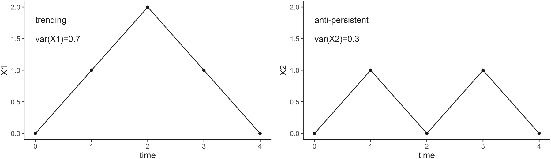
Simplified example: trending increments cause the variance of the cumulative return to grow faster, while anti-persistence has the opposite effect.
Both X 1 and X 2 will start and end at a value of 0, hence have the same expected return of zero. However, the former has a positive auto-correlation and the latter a negative one. We now see how the trending increments cause a larger variance for X 1, while variance does not grow for the anti-persistent X 2. Therefore, we recognize that variance of X grows faster under positive auto-correlation, while it grows slower when negative. This concept is key within the fractal analysis of time-series. If we further consider a 50 % chance that the signs of x 1, x 2 are inverted, then the expected values of X 1 and X 2 are zero for all t (and not just for t = 4). Hence, the term-structure of expected values does not necessarily tell whether expected auto-correlation is positive or negative.
A.2 The Rolling-Window Bias
To emphasize that estimating local return persistence is an econometrically not-so-obvious task I set up a simulation example similar to Bloch (2014). The main difficulty in estimating local serial dependence, as described in the main article, is the trade-off between sample size and estimation robustness. To illustrate the potential pitfalls I simulate three sub-paths of fractal Gaussian noise (see Mandelbrot and Van Ness 1968), each with a sample size of 500, but with serial-dependence of H = 0.65, 0.35 and 0.65. These simulations represent a stock’s daily log-returns, which are stacked together to create the overall time-series (see Figure A.2). The simulated series thus starts with trending returns, then jumps to anti-persistence, and then back to trending. Now, we are particularly interested in how different approaches perform in recognizing the actual change in the persistence structure. For this horse race I will compare the MF-DFA as implemented within the paper to rolling-window routines of classic R/S (Hurst 1956) and to rolling one-lag Pearson’s correlations
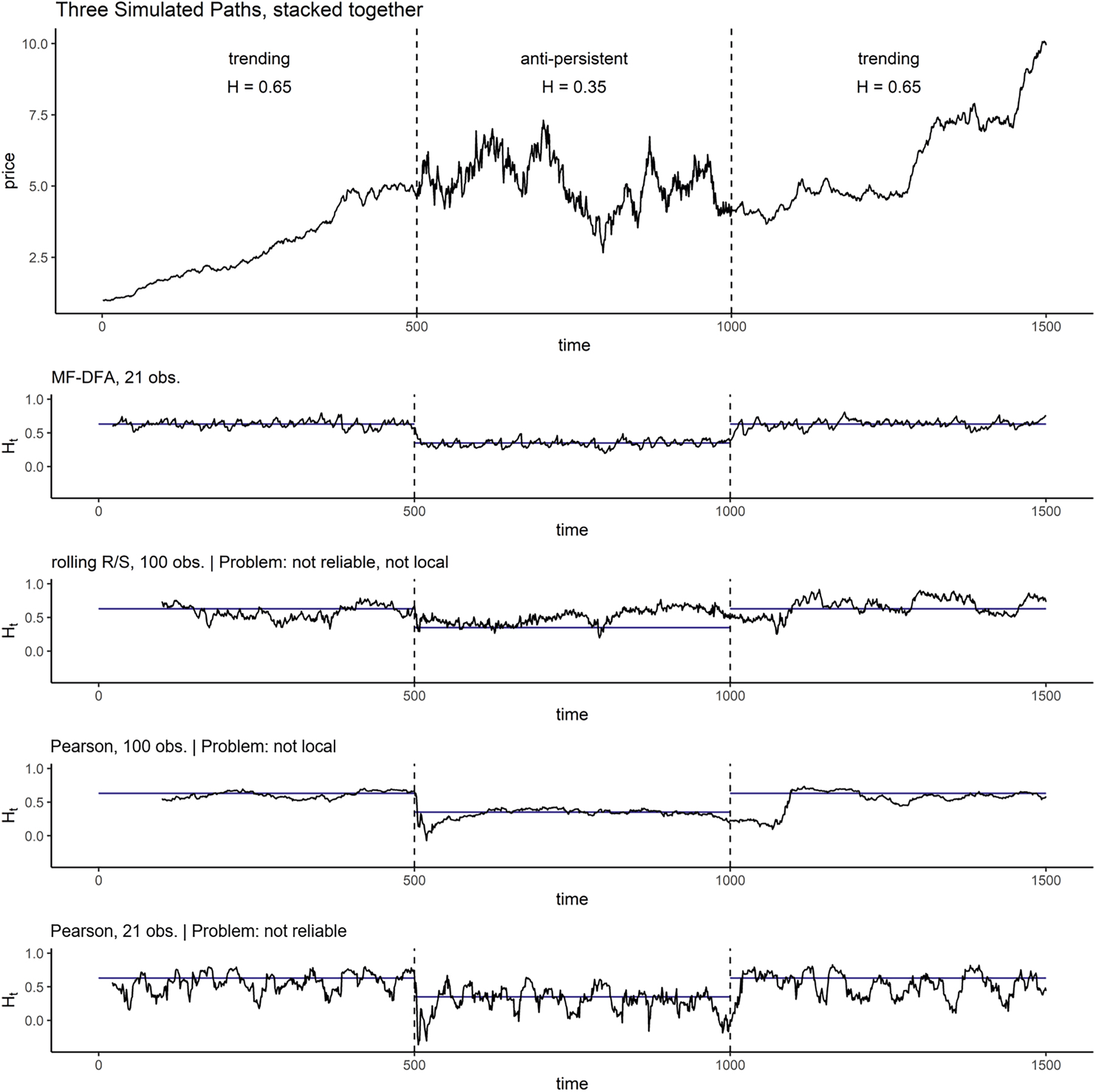
Upper plot: simulation of three return series (fractal Gaussian noise) with Hurst exponents of 0.65, 0.35 and 0.65, stacked together to an overall price path. Lower plots: comparison between various approaches for estimating local persistence H t . The difficulty is to find a balance between numerical reliability (more observations) and locality (fewer observations). The MF-DFA approach turns out to be the only one to find that balance. Blue lines indicate the segment’s overall H.
For the MF-DFA I will use a window size of 5–21 days. To make the rolling-window R/S competitive in terms of locality, I halve the recommended observation number down to a window-size of 100.[8] This makes the estimated H t numerically less reliable, but we hope to faster observe the change in true H. For the rolling Pearson analysis I choose two window-sizes. First, a size of 100 observations, such that the estimated correlation coefficients are reliable. Second, a window of 21 observations, which will be similarly local as the MF-DFA method. All methods will report right-aligned H t estimates, hence incorporate historical returns only.
The various H
t
estimates are visualized within the lower plots of Figure A.2. Let us study the results method by method. The MF-DFA approach uses a small time-window, hence can be considered to reflect local behavior. We observe this statement to hold upon the simulated series as the H
t
estimate adopts quickly to the change from the trending to the anti-persistent regime, and at the change back to the trending regime. Note that it is natural for empirical mono-fractal sequences, such as the simulated sub-paths, to have small fluctuations in H
t
. Since MF-DFA’s H
t
estimates vary only modestly within each regime and are on average very close to the simulation threshold H, we can also assume them to be reliable. Therefore, MF-DFA has a very good performance in balancing the trade-off between reliability and locality. With an eye on the rolling R/S analysis, we shall observe that the very opposite is the case. Here, the H
t
deviates much stronger from the true H level. Hence, the R/S fails to provide reliable persistence estimates. Especially at the switch from H = 0.35 to H = 0.65 we can further observe that the rolling window method also takes a long time to recognize the true change in persistence. As a consequence, the rolling-window routine is also improper in terms of capturing local correlation behavior. A similarly long-passage of time can be recognized at the Pearson correlation
Comparison of MF-DFA to rolling-window methods: setting and associated problems.
| Method | Window-size | SSE | Problem |
|---|---|---|---|
| MF-DFA | 21 | 5.12 | – |
| Rolling R/S | 100 | 28.32 | Window too short for reliable H t estimates. Also, window too large to reflect current behavior. |
| Pearson | 100 | 10.88 | Window too large to reflect current behavior. |
| Pearson | 21 | 48.97 | Window too short for reliable H t estimates. |
A.3 Economic Significance
The economic significance of serial-dependence is assessed upon simulated series of mono-fractal sequences for different levels of ρ. Simulations are made for ρ ∈ [−0.25, 0.25] with an interim step size of 0.01. For each level of ρ I simulate 103 many mono-fractal series with a length of 1,024 observations/days. Each simulation is then back-tested for a correlation-bet. This strategy expects a positive return for t + 1 if {r t , ρ t > 0} (continuation) or if {r t , ρ t < 0} (reversal). The strategy invests 1 when expected returns are positive, and −1 if negative. Transaction costs are considered in the size of 1.25 basis points, following the report of CME Group (2016). The mean return of the simulations is set to zero and standard deviation to 0.2 (annual). The benchmark for the strategy will be a long-only investment, which has by construction a mean return of 0. Therefore, I will use the mean return to assess whether the strategy is able to create value or not. Given that the strategy is a pure correlation bet, its profitability will rise the greater the serial-dependence ρ deviates from 0. The output of this simulation analysis is summarized in Figure A.3. I define economic significance as the level of ρ from which on the correlation-bet out-performs the benchmark in 95 % of the cases. These levels of economic significance are found at ρ = ±0.10.
![Figure A.3:
Estimating the level of serial-dependence ρ from which on it is profitable to make auto-correlation bets. Each bar plot summarizes the strategy’s mean return for 103 many simulations at a specific level of ρ. The blue points indicate the lowest 5 % of returns. The analysis indicates that serial-dependence ρ is economically significant whenever it is outside the [−0.10, 0.10] range.](/document/doi/10.1515/snde-2025-0099/asset/graphic/j_snde-2025-0099_fig_008.jpg)
Estimating the level of serial-dependence ρ from which on it is profitable to make auto-correlation bets. Each bar plot summarizes the strategy’s mean return for 103 many simulations at a specific level of ρ. The blue points indicate the lowest 5 % of returns. The analysis indicates that serial-dependence ρ is economically significant whenever it is outside the [−0.10, 0.10] range.
A.4 Crash Density
This section provides a brief analysis of the linkage between the serial correlation structure and market crashes, visualized in Figure A.4. The procedure behind the figure is as follows. The first step is to compute the empirical 5 % Value-at-Risk (VaR) of the daily log-returns. Next, we are interested into the level of ρ t and the probability that the next day return will be worse than the overall VaR. To assess this density, ρ t is classified into intervals of length 0.04 with exception to the outer ones being broader to capture at least 50 observations. The ρ t intervals are thus {[−0.47, − 0.32), [−0.32, − 0.28), [−0.28, − 0.24), …, [0.44, 0.52]}. Then, for each interval, I have computed the density of next day returns being worse than the VaR. This allows the following interpretation. In the case that crashes would be independent of ρ t , then the density should be constant at 5 %. However, Figure A.4 contradicts this statement. We can observe a convex pattern: the lower ρ t , the greater the probability for the next day return to be worse than the overall VaR. This means that market crashes are more likely to occur for low levels of expected auto-correlation ρ t . Following this interpretation, the measure becomes an interesting metric for the stability of financial markets.
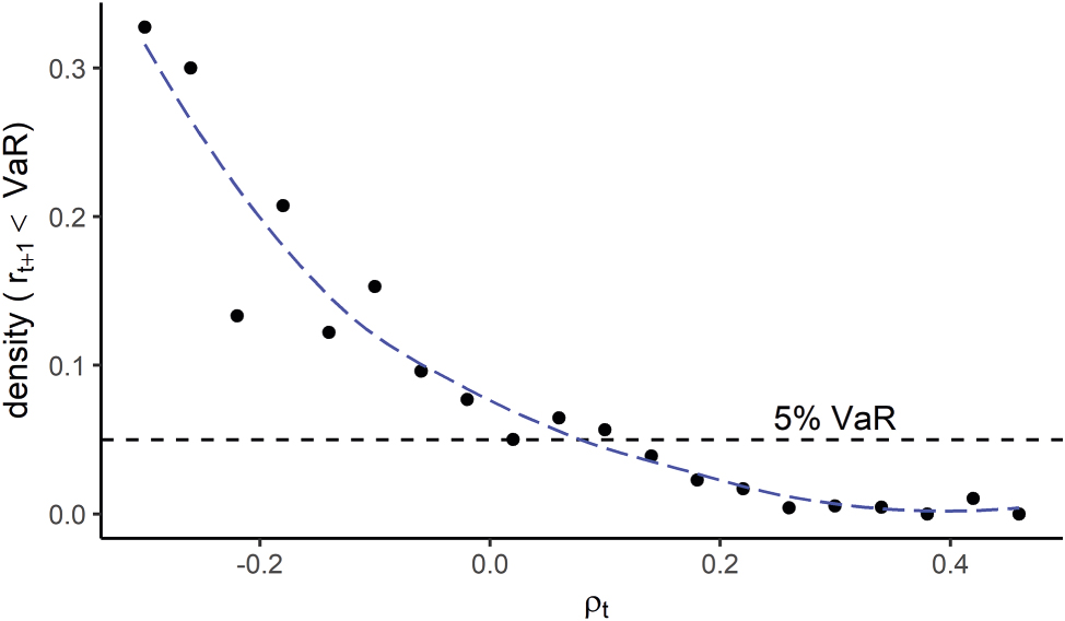
Density of the t + 1 return to be worse than the overall 5 % Value-at-Risk with respect to expected auto-correlation ρ t . The convex pattern can be interpreted as future crashes are more likely to occur when ρ t is low.
A.5 Implied versus Future-Realized Auto-Correlation
See Figure A.5
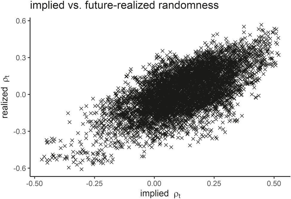
The S&P 500’s time-conditional serial-dependence as implied by option prices versus its future realization. The relationship appears to be well approximated under a linear model.
References
Aït-Sahalia, Y., M. Karaman, and L. Mancini. 2020. “The Term Structure of Equity and Variance Risk Premia.” Journal of Econometrics 219 (2): 204–30. https://doi.org/10.1016/j.jeconom.2020.03.002.Search in Google Scholar
Al-Yahyaee, K. H., W. Mensi, and S.-M. Yoon. 2018. “Efficiency, Multifractality, and the Long-Memory Property of the Bitcoin Market: A Comparative Analysis with Stock, Currency, and Gold Markets.” Finance Research Letters 27: 228–34. https://doi.org/10.1016/j.frl.2018.03.017.Search in Google Scholar
Ali, U., and D. Hirshleifer. 2020. “Shared Analyst Coverage: Unifying Momentum Spillover Effects.” Journal of Financial Economics 136 (3): 649–75. https://doi.org/10.1016/j.jfineco.2019.10.007.Search in Google Scholar
Aloui, C., S. J. H. Shahzad, and R. Jammazi. 2018. “Dynamic Efficiency of European Credit Sectors: A Rolling-Window Multifractal Detrended Fluctuation Analysis.” Physica A: Statistical Mechanics and its Applications 506: 337–49. https://doi.org/10.1016/j.physa.2018.04.039.Search in Google Scholar
Anderson, N., and J. Noss. 2013. “The Fractal Market Hypothesis and its Implications for the Stability of Financial Markets.” Bank of England Financial Stability Paper (23).Search in Google Scholar
Bachelier, L. 1900. “Théorie de la spéculation.” Annales Scientifiques de l’Ecole Normale Superieure 17: 21–86. https://doi.org/10.24033/asens.476.Search in Google Scholar
Baillie, R. T., T. Bollerslev, and H. O. Mikkelsen. 1996. “Fractionally Integrated Generalized Autoregressive Conditional Heteroskedasticity.” Journal of Econometrics 74 (1): 3–30. https://doi.org/10.1016/s0304-4076(95)01749-6.Search in Google Scholar
Barberis, N., R. Greenwood, L. Jin, and A. Shleifer. 2015. “X-capm: An Extrapolative Capital Asset Pricing Model.” Journal of Financial Economics 115 (1): 1–24. https://doi.org/10.1016/j.jfineco.2014.08.007.Search in Google Scholar
Batten, J. A., H. Kinateder, and N. Wagner. 2014. “Multifractality and Value-at-Risk Forecasting of Exchange Rates.” Physica A: Statistical Mechanics and its Applications 401: 71–81. https://doi.org/10.1016/j.physa.2014.01.024.Search in Google Scholar
Bayer, C., P. Friz, and J. Gatheral. 2016. “Pricing under Rough Volatility.” Quantitative Finance 16 (6): 887–904. https://doi.org/10.1080/14697688.2015.1099717.Search in Google Scholar
Bhardwaj, G., and N. R. Swanson. 2006. “An Empirical Investigation of the Usefulness of Arfima Models for Predicting Macroeconomic and Financial Time Series.” Journal of Econometrics 131 (1–2): 539–78. https://doi.org/10.1016/j.jeconom.2005.01.016.Search in Google Scholar
Bianchi, S., and M. Frezza. 2017. “Fractal Stock Markets: International Evidence of Dynamical (in) Efficiency.” Chaos: An Interdisciplinary Journal of Nonlinear Science 27 (7): 71102. https://doi.org/10.1063/1.4987150.Search in Google Scholar PubMed
Blanchard, O. 2009. “(Nearly) Nothing to Fear but Fear Itself.” The Economist, https://www.economist.com/finance-and-economics/2009/01/29/nearly-nothing-to-fear-but-fear-itself.Search in Google Scholar
Bloch, D. A. 2014. “A Practical Guide to Quantitative Portfolio Trading (SSRN Scholarly Paper No. 2543802).” SSRN Electronic Journal, https://doi.org/10.2139/ssrn.2543802.Search in Google Scholar
Bogachev, M. I., J. F. Eichner, and A. Bunde. 2007. “Effect of Nonlinear Correlations on the Statistics of Return Intervals in Multifractal Data Sets.” Physical Review Letters 99 (24): 240601. https://doi.org/10.1103/physrevlett.99.240601.Search in Google Scholar
Bollerslev, T., and V. Todorov. 2011. “Tails, Fears, and Risk Premia.” The Journal of Finance 66 (6): 2165–211. https://doi.org/10.1111/j.1540-6261.2011.01695.x.Search in Google Scholar
Bollerslev, T., G. Tauchen, and H. Zhou. 2009. “Expected Stock Returns and Variance Risk Premia.” Review of Financial Studies 22 (11): 4463–92. https://doi.org/10.1093/rfs/hhp008.Search in Google Scholar
Breeden, D. T., and R. H. Litzenberger. 1978. “Prices of State-Contingent Claims Implicit in Option Prices.” Journal of Business 51 (4): 621–51. https://doi.org/10.1086/296025.Search in Google Scholar
Britten-Jones, M., and A. Neuberger. 2000. “Option Prices, Implied Price Processes, and Stochastic Volatility.” The Journal of Finance 55 (2): 839–66. https://doi.org/10.1111/0022-1082.00228.Search in Google Scholar
Calvet, L. E., and A. J. Fisher. 2004. “How to Forecast Long-Run Volatility: Regime Switching and the Estimation of Multifractal Processes.” Journal of Financial Econometrics 2 (1): 49–83. https://doi.org/10.1093/jjfinec/nbh003.Search in Google Scholar
Caporale, G. M., L. Gil-Alana, and A. Plastun. 2018. “Is Market Fear Persistent? A Long-Memory Analysis.” Finance Research Letters 27: 140–7. https://doi.org/10.1016/j.frl.2018.02.007.Search in Google Scholar
Carr, P., and D. Madan. 2001. “Towards a Theory of Volatility Trading.” Option Pricing, Interest Rates and Risk Management, Handbooks in Mathematical Finance 22 (7): 458–76. https://doi.org/10.1017/cbo9780511569708.013.Search in Google Scholar
Castiglioni, P., and A. Faini. 2019. “A Fast DFA Algorithm for Multifractal Multiscale Analysis of Physiological Time Series.” Frontiers in Physiology 10: 115. https://doi.org/10.3389/fphys.2019.00115.Search in Google Scholar PubMed PubMed Central
Charles, A., and O. Darné. 2009. “Variance-Ratio Tests of Random Walk: An Overview.” Journal of Economic Surveys 23 (3): 503–27. https://doi.org/10.1111/j.1467-6419.2008.00570.x.Search in Google Scholar
Chen, S.-H., T. Lux, and M. Marchesi. 2001. “Testing for Non-Linear Structure in an Artificial Financial Market.” Journal of Economic Behavior & Organization 46 (3): 327–42. https://doi.org/10.1016/s0167-2681(01)00181-0.Search in Google Scholar
CME Group. 2016. “The Big Picture: A Cost Comparison of Futures and ETFs.” Technical Report.Search in Google Scholar
Cont, R. 2001. “Empirical Properties of Asset Returns: Stylized Facts and Statistical Issues.” Quantitative Finance 1 (2): 223–36. https://doi.org/10.1088/1469-7688/1/2/304.Search in Google Scholar
Cootner, P. H. 1964. The Random Character of Stock Market Prices. Cambridge: M.I.T. Press.Search in Google Scholar
Demeterfi, K., E. Derman, M. Kamal, and J. Zou. 1999. “A Guide to Volatility Swaps.” Journal of Derivatives 7: 9–32.10.3905/jod.1999.319129Search in Google Scholar
Ding, Z., C. W. J. Granger, and R. F. Engle. 1993. “A Long Memory Property of Stock Market Returns and a New Model.” Journal of Empirical Finance 1 (1): 83–106. https://doi.org/10.1016/0927-5398(93)90006-d.Search in Google Scholar
Drechsler, I., and A. Yaron. 2011. “What’s Vol Got to Do with It.” Review of Financial Studies 24 (1): 1–45. https://doi.org/10.1093/rfs/hhq085.Search in Google Scholar
Drozdz, S., J. Kwapien, P. Oswiecimka, and R. Rak. 2010. “The Foreign Exchange Market: Return Distributions, Multifractality, Anomalous Multifractality and the Epps Effect.” New Journal of Physics 12. https://doi.org/10.1088/1367-2630/12/10/105003.Search in Google Scholar
Elliott, R. J., and J. Van Der Hoek. 2003. “A General Fractional White Noise Theory and Applications to Finance.” Mathematical Finance 13 (2): 301–30. https://doi.org/10.1111/1467-9965.00018.Search in Google Scholar
Engle, R. F. 1982. “Autoregressive Conditional Heteroscedasticity with Estimates of the Variance of United Kingdom Inflation.” Econometrica 50 (4): 987–1007. https://doi.org/10.2307/1912773.Search in Google Scholar
Engle, R. F., and T. Bollerslev. 1986. “Modelling the Persistence of Conditional Variances.” Econometric Reviews 5 (1): 1–50. https://doi.org/10.1080/07474938608800095.Search in Google Scholar
Fama, E. F., and E. F. Fama. 1970. “Efficient Capital Markets: A Review of Theory and Empirical Work.” The Journal of Finance 25 (2): 383–417. https://doi.org/10.1111/j.1540-6261.1970.tb00518.x.Search in Google Scholar
Fama, E. F., and K. R. French. 1988. “Permanent and Temporary Components of Stock Prices.” Journal of Political Economy 96 (2): 246–73. https://doi.org/10.1086/261535.Search in Google Scholar
Frezza, M. 2014. “Goodness of Fit Assessment for a Fractal Model of Stock Markets.” Chaos, Solitons & Fractals 66: 41–50. https://doi.org/10.1016/j.chaos.2014.05.005.Search in Google Scholar
Gatheral, J., T. Jaisson, and M. Rosenbaum. 2018. “Volatility is Rough.” Quantitative Finance 18 (6): 933–49. https://doi.org/10.1080/14697688.2017.1393551.Search in Google Scholar
Ghazani, M. M., and R. Khosravi. 2020. “Multifractal Detrended Cross-Correlation Analysis on Benchmark Cryptocurrencies and Crude Oil Prices.” Physica A: Statistical Mechanics and its Applications 560: 125–72. https://doi.org/10.1016/j.physa.2020.125172.Search in Google Scholar
Gorski, A. Z., S. Drozdz, and J. Speth. 2002. “Financial Multifractality and its Subtleties: An Example of DAX.” Physica A: Statistical Mechanics and its Applications 316 (1–4): 496–510. https://doi.org/10.1016/s0378-4371(02)01021-x.Search in Google Scholar
Grech, D. 2016. “Alternative Measure of Multifractal Content and its Application in Finance.” Chaos, Solitons & Fractals 88: 183–95. https://doi.org/10.1016/j.chaos.2016.02.017.Search in Google Scholar
Grech, D., and Z. Mazur. 2004. “Can One Make Any Crash Prediction in Finance Using the Local Hurst Exponent Idea?” Physica A: Statistical Mechanics and its Applications 336 (1): 133–45. https://doi.org/10.1016/j.physa.2004.01.018.Search in Google Scholar
Green, E., W. Hanan, and D. Heffernan. 2014. “The Origins of Multifractality in Financial Time Series and the Effect of Extreme Events.” The European Physical Journal B 87 (6): 1–9. https://doi.org/10.1140/epjb/e2014-50064-x.Search in Google Scholar
Gu, D., and J. Huang. 2019. “Multifractal Detrended Fluctuation Analysis on High-Frequency SZSE in Chinese Stock Market.” Physica A: Statistical Mechanics and its Applications 521: 225–35. https://doi.org/10.1016/j.physa.2019.01.040.Search in Google Scholar
Hasan, R., and S. M. Mohammad. 2015. “Multifractal Analysis of Asian Markets During 2007–2008 Financial Crisis.” Physica A: Statistical Mechanics and its Applications 419: 746–61. https://doi.org/10.1016/j.physa.2014.10.030.Search in Google Scholar
Hou, A. J., and L. L. Nordén. 2018. “VIX Futures Calendar Spreads.” Journal of Futures Markets 38 (7): 822–38. https://doi.org/10.1002/fut.21886.Search in Google Scholar
Hu, Y., and B. Øksendal. 2003. “Fractional White Noise Calculus and Applications to Finance.” Infinite Dimensional Analysis, Quantum Probability and Related Topics 6 (1): 1–32.10.1142/S0219025703001110Search in Google Scholar
Hurst, H. E. 1956. “The Problem of Long-Term Storage in Reservoirs.” International Association of Scientific Hydrology. Bulletin 1 (3): 13–27. https://doi.org/10.1080/02626665609493644.Search in Google Scholar
Ihlen, E. 2012. “Introduction to Multifractal Detrended Fluctuation Analysis in Matlab.” Frontiers in Physiology 3: 141. https://doi.org/10.3389/fphys.2012.00141.Search in Google Scholar PubMed PubMed Central
Ihlen, E. A. F. 2013. “Multifractal Analyses of Response Time Series: A Comparative Study.” Behavior Research Methods 45 (4): 928–45. https://doi.org/10.3758/s13428-013-0317-2.Search in Google Scholar PubMed
Ihlen, E. A. F. 2014. Multifractal Analyses of Human Response Time: Potential Pitfalls in the Interpretation of Results.10.3389/fnhum.2014.00523Search in Google Scholar PubMed PubMed Central
Ihlen, E. A. F., and B. Vereijken. 2013. “Multifractal Formalisms of Human Behavior.” Human Movement Science 32 (4): 633–51. https://doi.org/10.1016/j.humov.2013.01.008.Search in Google Scholar PubMed
Ihlen, E. A. F., and B. Vereijken. 2014. “Detection of Co-Regulation of Local Structure and Magnitude of Stride Time Variability Using a New Local Detrended Fluctuation Analysis.” Gait & Posture 39 (1): 466–71. https://doi.org/10.1016/j.gaitpost.2013.08.024.Search in Google Scholar PubMed
Jiang, G. J., and Y. S. Tian. 2005. “The Model-Free Implied Volatility and its Information Content.” Review of Financial Studies 18 (4): 1305–42. https://doi.org/10.1093/rfs/hhi027.Search in Google Scholar
Jiang, Z.-Q., and W.-X. Zhou. 2008. “Multifractal Analysis of Chinese Stock Volatilities Based on the Partition Function Approach.” Physica A: Statistical Mechanics and its Applications 387 (19): 4881–8. https://doi.org/10.1016/j.physa.2008.04.028.Search in Google Scholar
Jiang, Z.-Q., W.-J. Xie, W.-X. Zhou, and D. Sornette. 2019. “Multifractal Analysis of Financial Markets: A Review.” Reports on Progress in Physics 82 (12): 125901. https://doi.org/10.1088/1361-6633/ab42fb.Search in Google Scholar PubMed
Kantelhardt, J. W., S. A. Zschiegner, E. Koscielny-Bunde, S. Havlin, A. Bunde, and H. Stanley. 2002. “Multifractal Detrended Fluctuation Analysis of Nonstationary Time Series.” Physica A: Statistical Mechanics and its Applications 316 (1): 87–114. https://doi.org/10.1016/s0378-4371(02)01383-3.Search in Google Scholar
Khashanah, K., and C. Shao. 2021. “Short-Term Volatility Forecasting with Kernel Support Vector Regression and Markov Switching Multifractal Model.” Quantitative Finance: 1–13. https://doi.org/10.1080/14697688.2021.1939116.Search in Google Scholar
Kristoufek, L., and M. Vosvrda. 2013. “Measuring Capital Market Efficiency: Global and Local Correlations Structure.” Physica A: Statistical Mechanics and its Applications 392: 184–93. https://doi.org/10.1016/j.physa.2012.08.003.Search in Google Scholar
Kristoufek, L., and M. Vosvrda. 2014. “Measuring Capital Market Efficiency: Long-Term Memory, Fractal Dimension and Approximate Entropy.” The European Physical Journal B 87 (162). https://doi.org/10.1140/epjb/e2014-50113-6.Search in Google Scholar
Kwapien, J., P. Oswiecimka, and S. Drozdz. 2005. “Components of Multifractality in High-Frequency Stock Returns.” Physica A: Statistical Mechanics and its Applications 350 (2–4): 466–74. https://doi.org/10.1016/j.physa.2004.11.019.Search in Google Scholar
Li, J., and G. Zinna. 2018a. “The Variance Risk Premium: Components, Term Structures, and Stock Return Predictability.” Journal of Business & Economic Statistics 36 (3): 411–25. https://doi.org/10.1080/07350015.2016.1191502.Search in Google Scholar
Li, J., and G. Zinna. 2018b. “The Variance Risk Premium: Components, Term Structures, and Stock Return Predictability.” Journal of Business & Economic Statistics 36 (3): 411–25. https://doi.org/10.1080/07350015.2016.1191502.Search in Google Scholar
Livieri, G., S. Mouti, A. Pallavicini, and M. Rosenbaum. 2018. “Rough Volatility: Evidence from Option Prices.” IISE Transactions 50 (9): 767–76. https://doi.org/10.1080/24725854.2018.1444297.Search in Google Scholar
Lo, A. W. 1991. “Long-Term Memory in Stock Market Prices.” Econometrica 59 (5): 1279–313. https://doi.org/10.2307/2938368.Search in Google Scholar
Lobato, I. N., and N. E. Savin. 1998. “Real and Spurious Long-Memory Properties of Stock-Market Data.” Journal of Business & Economic Statistics 16 (3): 261–8. https://doi.org/10.1080/07350015.1998.10524760.Search in Google Scholar
Lux, T., and S. Alfarano. 2016. “Financial Power Laws: Empirical Evidence, Models, and Mechanisms.” Chaos, Solitons & Fractals 88: 3–18. https://doi.org/10.1016/j.chaos.2016.01.020.Search in Google Scholar
Lux, T., and M. Ausloos. 2002. “Market Fluctuations I: Scaling, Multiscaling, and their Possible Origins.” In The Science of Disasters, 372–409. Springer.10.1007/978-3-642-56257-0_13Search in Google Scholar
Lux, T., and M. Segnon. 2018. Multifractal Models in Finance, Vol. 1. Oxford University Press.10.1093/oxfordhb/9780199844371.013.8Search in Google Scholar
Lux, T., M. Segnon, and R. Gupta. 2016. “Forecasting Crude Oil Price Volatility and Value-at-Risk: Evidence from Historical and Recent Data.” Energy Economics 56: 117–33. https://doi.org/10.1016/j.eneco.2016.03.008.Search in Google Scholar
Mandelbrot, B. B. 1963. “The Variation of Certain Speculative Prices.” Journal of Business 36 (4): 394–419. https://doi.org/10.1086/294632.Search in Google Scholar
Mandelbrot, B. B. 2013. Multifractals and 1/f Noise: Wild Self-Affinity in Physics (1963–1976). Springer.Search in Google Scholar
Mandelbrot, B. B., and J. W. Van Ness. 1968. “Fractional Brownian Motions, Fractional Noises and Applications.” SIAM Review 10 (4): 422–37. https://doi.org/10.1137/1010093.Search in Google Scholar
Mandelbrot, B. B., A. J. Fisher, and L. E. Calvet. 1997. A Multifractal Model of Asset Returns. Yale University. Cowles Foundation Discussion Paper No. 1164.Search in Google Scholar
Martin, I. 2011. “Simple Variance Swaps.” Technical Report.10.3386/w16884Search in Google Scholar
Martin, I. 2017. “What is the Expected Return on the Market?” Quarterly Journal of Economics 132 (1): 367–433. https://doi.org/10.1093/qje/qjw034.Search in Google Scholar
Martin, I. 2021. “On the Autocorrelation of the Stock Market*.” Journal of Financial Econometrics 19 (1): 39–52. https://doi.org/10.1093/jjfinec/nbaa033.Search in Google Scholar
Morales, R., T. Di Matteo, R. Gramatica, and T. Aste. 2012. “Dynamical Generalized Hurst Exponent as a Tool to Monitor Unstable Periods in Financial Time Series.” Physica A: Statistical Mechanics and its Applications 391 (11): 3180–9. https://doi.org/10.1016/j.physa.2012.01.004.Search in Google Scholar
Moyano, L. G., J. de Souza, and S. M. Duarte Queirós. 2006. “Multi-Fractal Structure of Traded Volume in Financial Markets.” Physica A: Statistical Mechanics and its Applications 371 (1): 118–21. https://doi.org/10.1016/j.physa.2006.04.098.Search in Google Scholar
Morelli, G., and P. Santucci de Magistris. 2019. “Volatility Tail Risk Under Fractionality.” Journal of Banking & Finance 108: 105654. https://doi.org/10.1016/j.jbankfin.2019.105654.Search in Google Scholar
Mukli, P., Z. Nagy, and A. Eke. 2015. “Multifractal Formalism by Enforcing the Universal Behavior of Scaling Functions.” Physica A: Statistical Mechanics and its Applications 417: 150–67. https://doi.org/10.1016/j.physa.2014.09.002.Search in Google Scholar
Neuberger, A. 2012. “Realized Skewness.” Review of Financial Studies 25 (11): 3423–55. https://doi.org/10.1093/rfs/hhs101.Search in Google Scholar
Peng, C.-K., S. V. Buldyrev, S. Havlin, M. Simons, H. E. Stanley, and A. L. Goldberger. 1994. “Mosaic Organization of DNA Nucleotides.” Physical Review E 49 (2): 1685–9. https://doi.org/10.1103/physreve.49.1685.Search in Google Scholar PubMed
Peters, E. E. 1989. “Fractal Structure in the Capital Markets.” Financial Analysts Journal 45 (4): 32–7. https://doi.org/10.2469/faj.v45.n4.32.Search in Google Scholar
Ray, B. K., and R. S. Tsay. 2000. “Long-Range Dependence in Daily Stock Volatilities.” Journal of Business & Economic Statistics 18 (2): 254–62. https://doi.org/10.1080/07350015.2000.10524867.Search in Google Scholar
Schadner, W. 2020. “An Idea of Risk-Neutral Momentum and Market Fear.” Finance Research Letters 37: 101347. https://doi.org/10.1016/j.frl.2019.101347.Search in Google Scholar
Schadner, W. 2021. “On the Persistence of Market Sentiment: A Multifractal Fluctuation Analysis.” Physica A: Statistical Mechanics and its Applications 581: 126242. https://doi.org/10.1016/j.physa.2021.126242.Search in Google Scholar
Schadner, W. 2022. “U.S. Politics from a Multifractal Perspective.” Chaos, Solitons & Fractals 155. https://doi.org/10.1016/j.chaos.2021.111677.Search in Google Scholar
Schreiber, T., and A. Schmitz. 2000. “Surrogate Time Series.” Physica D: Nonlinear Phenomena 142 (3): 346–82. https://doi.org/10.1016/s0167-2789(00)00043-9.Search in Google Scholar
Sensoy, A. 2013. “Generalized Hurst Exponent Approach to Efficiency in MENA Markets.” Physica A: Statistical Mechanics and its Applications 392 (20): 5019–26. https://doi.org/10.1016/j.physa.2013.06.041.Search in Google Scholar
Shahzad, S. J. H., S. M. Nor, W. Mensi, and R. R. Kumar. 2017. “Examining the Efficiency and Interdependence of US Credit and Stock Markets Through MF-DFA and MF-DXA Approaches.” Physica A: Statistical Mechanics and its Applications 471: 351–63. https://doi.org/10.1016/j.physa.2016.12.037.Search in Google Scholar
Shahzad, S. J. H., J. A. Hernandez, W. Hanif, and G. M. Kayani. 2018. “Intraday Return Inefficiency and Long Memory in the Volatilities of Forex Markets and the Role of Trading Volume.” Physica A: Statistical Mechanics and its Applications 506: 433–50. https://doi.org/10.1016/j.physa.2018.04.016.Search in Google Scholar
Sias, R. W., and L. T. Starks. 1997. “Return Autocorrelation and Institutional Investors.” Journal of Financial Economics 46 (1): 103–31. https://doi.org/10.1016/s0304-405x(97)00026-3.Search in Google Scholar
Szakmary, A., E. Ors, J. K. Kim, and W. N. Davidson Iii. 2003. “The Predictive Power of Implied Volatility: Evidence from 35 Futures Markets.” Journal of Banking & Finance 27 (11): 2151–75. https://doi.org/10.1016/s0378-4266(02)00323-0.Search in Google Scholar
Tan, Z., J. Liu, and J. Chen. 2021. “Detecting Stock Market Turning Points Using Wavelet Leaders Method.” Physica A: Statistical Mechanics and its Applications 565. https://doi.org/10.1016/j.physa.2020.125560.Search in Google Scholar
Traut, J., and W. Schadner. 2023. Which is Worse: Heavy Tails or Volatility Clusters? Swiss Finance Institute Research Paper, 23–61.10.2139/ssrn.4410908Search in Google Scholar
Turiel, A., and C. J. Pérez-Vicente. 2005. “Role of Multifractal Sources in the Analysis of Stock Market Time Series.” Physica A: Statistical Mechanics and its Applications 355 (2): 475–96. https://doi.org/10.1016/j.physa.2005.04.002.Search in Google Scholar
Yan, R., D. Yue, X. Chen, and X. Wu. 2020. “Non-Linear Characterization and Trend Identification of Liquidity in China’s New OTC Stock Market Based on Multifractal Detrended Fluctuation Analysis.” Chaos, Solitons & Fractals 139: 110063. https://doi.org/10.1016/j.chaos.2020.110063.Search in Google Scholar
Zhou, W.-X. 2009. “The Components of Empirical Multifractality in Financial Returns.” Europhysics Letters 88 (2): 28004. https://doi.org/10.1209/0295-5075/88/28004.Search in Google Scholar
Supplementary Material
This article contains supplementary material (https://doi.org/10.1515/snde-2025-0099).
© 2025 Walter de Gruyter GmbH, Berlin/Boston