Have European natural gas prices decoupled from crude oil prices? Evidence from TVP-VAR analysis
-
Karol Szafranek
 and
Michał Rubaszek
and
Michał Rubaszek

Abstract
Unprecedented increases in European natural gas prices observed between late 2021 and mid 2022 raise a question about the sources of these events. In this article we investigate this topic using a time-varying parameters structural vector autoregressive model for crude oil, US and European natural gas prices. This flexible framework allows us to measure how disturbances specific to the analyzed markets propagate within the system and how this propagation mechanism evolves in time. Our findings are fourfold. First, we show that oil prices are hardly affected by shocks specific to natural gas markets, whether in the US or Europe. Second, we demonstrate that oil shocks have limited impact on US natural gas prices, which points to the decoupling of both markets. Third, we evidence that over longer horizons natural gas prices in Europe are still mostly determined by oil shocks, with idiosyncratic disturbances leading to short-lived decoupling of both commodity prices. Fourth, we illustrate that along the gradual shift from oil price indexation to gas-on-gas competition, the contribution of idiosyncratic shocks to European natural gas prices has increased. Nonetheless, we discuss why the notion that EU natural gas and crude oil prices have decoupled might be premature.
1 Introduction
The broad aim of this article is to understand the main drivers of natural gas prices in Europe, which is important as this commodity is a strategic source of energy in the most European countries. It plays a crucial role in residential and commercial heating, serves as an important input for industrial production and represents a significant part of electricity generation mix. In general, natural gas is considered to be a bridge fuel in energy transition, as gas power plants emit much less carbon dioxide than coal plants and due to their dispatchability are a far better complement to unstable renewable energy sources. These features have been recognized by the European Commission, which labelled natural gas as a green energy source that be can exploited by countries in their transition to a low-carbon economy. For the above reasons the unprecedented increase in prices of this commodity observed between the second half of 2021 and August 2022 across European hubs, which was related to the Russian invasion of Ukraine, constituted a significant disturbance to the functioning of the European economy. First, it has generated considerable inflationary pressure, thus posing risk to the economic recovery following the outbreak of the Covid-19 pandemic and leading to downward revisions of economic outlook for major European economies. Second, it has raised fundamental concerns with respect to Europe’s energy security, a topic already described in details in the academic literature (Bouwmeester and Oosterhaven 2017; Rodriguez-Gomez et al. 2016). Third, it has changed estimated costs of decarbonization policy.
The important role of natural gas as a source of energy is also reflected in the academic literature by a high number of studies attempting to explain the dynamics of its prices (see Table 1). They usually point to the fact that the global natural gas market is geographically segmented into several local markets due to transportation costs and the presence of heterogeneous institutions (see Kan et al. 2019, for a detailed overview of the global natural gas market structure). Consequently, natural gas prices evolve fairly independently in different parts of the world, especially after the shale gas revolution in the US (Geng et al. 2016b; Wakamatsu and Aruga 2013; Zhang and Ji 2018). On the contrary, local natural gas markets connected by pipelines, i.e. the European ones, are closely integrated (Broadstock et al. 2020; Papiez et al. 2022). This distinguishes natural gas from crude oil, which prices are determined by global rather than local factors. This dichotomy in terms of geographical coverage, combined with the fact that both energy commodities are imperfect substitutes, has motivated researchers to investigate the relationship among the dynamics of regional natural gas and global crude oil prices. One of the conclusions is that the natural gas market is strongly influenced by the developments in the crude oil market, with little evidence for reverse causality (Gong et al. 2021; Jadidzadeh and Serletis 2017; Lin and Li 2015; Tiwari et al. 2019).[1] Additionally, some authors indicate that the long-term relationship between both commodities in the US market has decoupled since mid 2000s, which did not happen in the European market (Erdos 2012; Geng et al. 2016a; Siliverstovs et al. 2005; Zhang and Ji 2018).
Survey of studies on joint dynamics of energy commodity markets.
| Authors (year) | Method | Findings |
|---|---|---|
| Integration of CO and NG markets | ||
| Siliverstovs et al. (2005) | VEC | Long-run link between European and Asian NG markets, but no long-run link with US NG prices over 1990–2004. |
| Brown and Yucel (2009) | VEC | Long-run link between US and UK NG prices over 1997–2008 driven by CO prices rather than GoG competition. |
| Erdos (2012) | VEC | Long-run NG-CO link both in US and UK until 2009, but decoupling of US NG afterwards. |
| Wakamatsu and Aruga (2013) | Cointegration test | Decoupling of US and Japanese NG markets after 2005. |
| Nick and Thoenes (2014) | Structural VAR | European NG price fluctuations driven by idiosyncratic factors at short run, but CO and coal prices in longer horizons. |
| Geng et al. (2016b) | MS-AR | US NG decoupled from CO prices, while UK NG and CO prices were cointergarted over 1998 to 2015. |
| Jadidzadeh and Serletis (2017) | Structural VAR | CO market shocks explain 45 % of US NG price fluctuations over 1976–2012. |
| Asche et al. (2017) | MS-VEC | NG prices in UK and CO prices were cointegrated over years 1997–2014 if one accounts for regime shifts. |
| Zhang and Ji (2018) | Fractional integration | Long-run link between CO and NG prices for Europe and Asia, but not for US over 1982–2015. |
| TVP models applied to energy commodity markets | ||
| Baumeister and Peersman (2013) | TVP-VAR | The importance of oil supply shocks for real oil price variability decreases in contrast to oil demand shocks. |
| Batten et al. (2017) | Rolling VAR | Rolling window estimates over 1994–2014 indicate that till 2006 US NG prices were Granger causing CO prices. |
| Wiggins and Etienne (2017) | TVP-VAR | US NG market dynamics over 1993–2015 well described by a model with slowly changing coefficients and big changes in volatility. |
| Liu and Gong (2020) | TVP-VAR | Spillovers between four major crude oil markets indicate slowly increasing connectedness with cyclical dependence. |
| Gao et al. (2021) | Univariate TVP | Models with small changes in coefficients and big in volatility deliver competitive forecasts for NG prices in Europe, Japan and US over 1992–2019. |
| Gong et al. (2021) | TVP-VAR | A model with small changes in coefficients and big in volatility well describes joint dynamics of CO, NG, gasoline and HO in US over 2005–2019. |
| Anand and Paul (2021) | TVP-VAR | Impact of global economic policy uncertainty shocks are frequently amplified during extreme market events. The response of Brent and WTI crude oil prices to these shocks can differ. |
| Ding et al. (2021) | TVP-VAR | Volatility of commodity futures respond differently to different types of financial uncertainty shocks |
| Lyu et al. (2021) | TVP-VAR | Effects of global economic policy uncertainty shocks on crude oil prices increase during periods of crisis. |
| Shang and Hamori (2021) | TVP-VAR | WTI has greater spillover effects on the exchange rates of oil-importing countries. |
| Papiez et al. (2022) | TVP-VAR | TVP-VAR well describes joint dynamics of NG prices in European hubs over 2013–2022. |
-
NG, natural gas; CO, crude oil; HO, heating oil; AR, autoregressive model; VAR, vector autoregressive model; VEC, vector error correction model; TVP, time-varying parameter; MS, Markov switching.
Another widely discussed issue in the literature concerns the source of natural gas price fluctuations. The authors usually focus on the US market and apply the structural vector autoregression (VAR) framework. One of the reasons is that the natural gas market in the US was the first one that was fully deregulated following the Natural Gas Policy Act of 1978. Consequently, since mid-1990s natural gas prices have been entirely determined by market forces (Joskow 2013). This justifies the application of dynamic models in which prices of this commodity are driven by supply and demand factors. The studies using structural VAR models point to three regularities. First, demand shocks seem more important in explaining the dynamics of natural gas prices rather than supply shocks (Arora and Lieskovsky 2014; Hailemariam and Smyth 2019; Hou and Nguyen 2018; Rubaszek et al. 2021). Second, the dynamics of the US natural gas market is not stable over time (Hou and Nguyen 2018; Nguyen and Okimoto 2019; Rubaszek and Uddin 2020; Rubaszek et al. 2020; Wiggins and Etienne 2017), which justifies the use of time-varying parameters models as postulated by Granger (2008). Third, natural gas prices are affected by oil prices with little reverse causality (Jadidzadeh and Serletis 2017).
Against this background, the price formation mechanism on the European natural gas market is relatively unexplored. This might be related to the fact that modelling this market is challenging for two reasons. First, the analysis of supply requires taking into account that it was predominantly based on imports via pipelines from Russia. According to Eurostat, the EU’s reliance on gas imports from Russia stood at almost 40 % in 2020. Other import directions via pipelines include mostly Norway and Algeria. The demand is further balanced by domestic sources and an increasing share of liquefied natural gas (LNG). It should be noted, however, that over time the role of domestic sources has declined, with decreasing supply from the UK and the Netherlands, while the LNG market has experienced a significant development over the last decades and is forecast to grow even stronger, given the EU’s pledge to limit Russian imports. This evolution may reinforce the linkages between distant gas markets, leading to the convergence of prices across Atlantic (Mu and Ye 2018). Nonetheless, the existing import-based supply has not only raised energy security questions (Bouwmeester and Oosterhaven 2017; Rodriguez-Gomez et al. 2016), but also makes it difficult to assess supply response to economic factors.
The second challenge in modelling the European natural gas market is related to the fact that it has undergone the liberalization process only over the last two decades. This involved several legislative packages, which are described in details by Bastianin et al. (2019). In 1998, the First Gas Directive opened up the market to competition by facilitating the entry into the competitive segments of the industry (transmission, distribution, supply and storage). In 2003, the Second Gas Directive unbundled transmission from supply. In 2009, the Third Gas Directive introduced common rules for the functioning of natural gas market, including incentives for launching trading hubs. These changes have resulted in a gradual but sizeable shift from oil price indexation (OPI) to gas-on-gas (GoG) competition (Chyong 2019; del Valle et al. 2017; Stern 2014). According to IGU (2021), between 2005 and 2020 the share of GoG contracts in total gas consumption increased from 15 % to 80 %, whereas the share of OPI went down from 78 % to 20 %.
The above developments urge the question on whether European natural gas prices are still driven by changes in oil prices or rather the role of US natural gas prices and fundamental factors specific to the European natural gas market has increased over time. So far this question has been only partially answered in the literature. A number of studies applied cointegration techniques in search for the long-term relationship between oil and natural gas prices in the US and in Europe (see Ji et al. 2018, for a comprehensive survey). Specifically, Brown and Yucel (2009) conclude that the co-movement between European and US natural gas prices is driven by crude oil prices rather than gas-to-gas arbitrage across the Atlantic. In turn, Asche et al. (2017) show that European natural gas prices and Brent oil prices are cointegrated, but the long-term relationship is regime dependent. The authors also claim that in GoG markets the relationship between oil and natural gas prices should be weaker as natural gas should be priced as a unique commodity. This kind of result is presented for the US, but not for Europe (Erdos 2012). However, it can be expected that a similar decoupling will be observed in Europe, given the ongoing shift towards the GoG pricing model. In this respect, two studies should be mentioned. Nick and Thoenes (2014) propose a structural VAR model to show that natural gas prices in Germany are affected by temperature, storage and supply shortfalls in the short-term, while in the long-term they are tied to crude oil and coal prices. Hulshof et al. (2016) find that daily spot prices at the Dutch Title Transfer Facility (TTF) hub are over short-term horizon only mildly affected by changes in oil prices, but react to European idiosyncratic factors such as the level of natural gas inventories, temperature and the production of wind electricity.
There are also a few very recent studies indicating that the impact of oil prices on the natural gas market should be analyzed using time-varying parameters (TVP) framework (see Table 1). For instance, Wiggins and Etienne (2017) show that the TVP-VAR model can be successfully applied to describe the dynamics of the US natural gas market. Gong et al. (2021) estimate a TVP-VAR model to investigate dynamic volatility spillovers between four major energy commodities (crude oil, gasoline, heating oil and natural gas) in the US market. Ji et al. (2018) employ a model with time-varying parameters (estimated in a rolling window) to analyze the oil–gas relationship within the connectedness network framework. In turn, Gao et al. (2021) show that univariate models allowing for gradual changes in coefficients and drastic changes in volatility have the best forecasting performance for European gas prices. Finally, Papiez et al. (2022) indicate that a TVP-VAR model can be applied to describe the joint dynamics of natural gas prices at major European hubs. These studies clearly show that the changing structure of the natural gas market requires the use of models with time-varying parameters. Table 1 also indicates that the popularity of the TVP-VAR framework in analysing the dynamics of energy commodity markets has increased in recent years.
In this work, we contribute to the above studies by investigating how changes in oil and natural gas prices in the US affect natural gas prices in Europe. We start by estimating a constant coefficient structural VAR model for the three variables. Based on this framework we analyze the determinants of European natural gas prices using impulse response functions, forecast error variance decomposition and historical decomposition. Next, given the gradually changing structure of the European natural gas market we relax our key model assumption on parameters being constant over the entire sample and move to the time-varying parameters model with stochastic volatility (henceforth TVP-VAR-SV). This approach allows us to examine the evolving relationship between oil prices, US natural gas prices and European natural gas prices at each point in time.
Our study allows us to make two general conclusions. The constant coefficient framework indicates that over the entire sample the dynamics of natural gas prices in Europe was driven predominantly by local factors over the short-run, but their importance decreases in the medium and long-term horizon as oil shocks account for up to around 55 % of EU natural gas prices variability. On the contrary, natural gas prices in the US evolved fairly independently of the developments in the oil market. Consequently, natural gas prices were also decoupled across the Atlantic. This outcome confirms the prevailing evidence in the literature. Next, the TVP-VAR-SV analysis demonstrates that over the last two decades, with the ongoing shift from OPI to GoG structure, the contribution of local shocks to European natural gas prices fluctuations has gradually increased in time. However, despite this trend, in the long-term European gas prices are still determined mostly by the developments in the crude oil market. The TVP-VAR-SV model also shows that the most recent developments, i.e. drastic natural gas prices increases, can be explained by increased volatility of local shocks rather than by the decoupling from the oil market. We believe that these results provide a new insight into the discussion on the dynamics of the European natural gas market.
The remainder of the article is structured as follows. Section 2 describes the data. In Section 3 we present the constant coefficient structural VAR model and discuss the results. In Section 4 we move to the time-varying parameters framework and investigate the interplay between the energy commodity prices in time. Section 5 grants conclusions and policy implications.
2 Data
Our analysis is based on monthly data from January 1993 to October 2022, a sample that covers the period in which the US natural gas market was deregulated. We also use data from January 1983 to December 1992 for technical purposes, i.e. as a pre-sample to calibrate prior information for the TVP-VAR-SV model. It can be noted that this choice is standard for studies focused on the US market surveyed above, e.g. the work by Wiggins and Etienne (2017).
We take nominal prices of WTI crude oil (P OIL) as well as US and EU natural gas (P NGUS and P NGEU) from the World Bank commodity database. These three variables are usually expressed in different units of measure, namely USD per barrel, USD per MMBtu and EUR per MWh. For the sake of comparability, we express them in the common unit, i.e. USD per barrel of oil equivalent (boe). Next, we deflate them using the US consumer price index, taken from the FRED database, which we rescale so that its value for the last observation (October 2022) is equal to unity. Consequently, all real prices are expressed in units from the end of the sample. Finally, all the series were adjusted for seasonal patters, which – although weak – were present, especially in the case of natural gas.
A quick look at the series presented in Figure 1 warrants few observations. First, oil and natural gas prices are visibly correlated, with the link stronger for the EU than the US market. In general, over almost the entire sample EU natural gas prices follow oil prices, which might reflect their partial indexation within long-term contracts. Second, the volatility of natural gas prices in the US tends to be higher than in Europe, which might reflect different structures of both markets. However, since the second half of 2021 until August 2022 we observe a striking increase in European gas prices, by far outpacing changes in the remaining two variables. Third, all the series experience periods of higher and lower variability, which would suggest that a robust model describing these markets should take into account that the volatility of shocks is time-varying.

Time series for the prices of oil and natural gas in the US and Europe. The figure presents the development in real oil and natural gas prices over the main sample. For the sake of comparability, all series are expressed in USD per barrel of oil equivalent. The y-axis is put in logarithmic scale.
The above visual characteristics of the data presented in Figure 1 are complemented by descriptive statistics in Table 2. It shows that log changes in European gas prices are less volatile that the remaining series, leptokurtic and slightly autocorrelated. We also find that the ADF test fails to reject the null for the log levels of all the series. However, this outcome can be attributed to the low power of the test for persistent variables. In our modeling framework we proceed with log levels of real prices of the analyzed variables as is usually done in structural VAR models for oil and natural gas (e.g. Jadidzadeh and Serletis 2017; Kilian 2009).
Descriptive statistics for the real prices of oil and natural gas in the US and in Europe.
| ADF | Moments | ACF | |||||||||
|---|---|---|---|---|---|---|---|---|---|---|---|
| Level | Diff | Min | Mean | SD | Max | Skew. | Kurt. | Lag 1 | Lag 2 | LB | |
| OIL | −2.06 | −11.09 | −57.49 | 2.61 | 31.73 | 55.18 | −0.81 | 13.20 | 0.21 | −0.03 | 0.000 |
| NGUS | −2.60 | −11.39 | −65.33 | 0.98 | 47.73 | 66.19 | 0.17 | 6.25 | −0.02 | −0.06 | 0.493 |
| NGEU | −1.51 | −7.16 | −52.74 | 5.41 | 30.09 | 48.09 | −0.03 | 12.28 | 0.22 | 0.03 | 0.000 |
-
The table presents the descriptive statistics for monthly log changes (in per cent) in real oil and natural gas prices calculated on the main sample. The specification of the Augmented Dickey-Fuller (ADF) test includes a constant and two lags. The 1 % and 5 % critical values are −3.44 and −2.87, respectively. The mean and standard deviation is presented in annualized terms. ACF stands for autocorrelation coefficients and LB for the p-value of the Ljung-Box test with the null of no autocorrelation for the first two lags.
3 Constant coefficient structural VAR approach
3.1 The model
We start our investigation of the European natural gas market by considering a structural VAR model for the trivariate vector
where B 0 is a 3 × 1 vector of constant terms, B i for i = 1, 2, …, l denote 3 × 3 matrices of autoregressive coefficients, D is a 3 × 3 identification matrix and η t is a 3 × 1 vector of structural shocks. It contains innovations to US oil (η OIL), US natural gas (η NGUS) and EU natural gas (η NGEU) prices. In model identification, we impose the recursive identification scheme, in which D is a lower triangular matrix as:
Based on the Schwarz information criterion, we set the maximum lag to l = 2 and estimate the reduced-form VAR on the main sample with the least squares method. Next, we use the estimated covariance matrix of residuals to compute the elements
3.2 The results
Impulse response functions. Figure 2 presents the impulse response functions (IRFs) of endogenous variables to one standard deviation of structural shocks along with the 90 % confidence bands. The left top panel illustrates that an oil market innovation immediately leads to an increase in crude oil prices by 9 %, which in the subsequent two months reaches a peak of almost 11 %. After the initial jump, oil prices slowly return to equilibrium, but even after five years their level is still around 3 % above the level observed before the occurrence of the shock. The center top panel demonstrates that oil prices are not significantly affected by shocks to US natural gas prices, which confirms the earlier results in the surveyed literature (e.g. Jadidzadeh and Serletis 2017). The right top panel shows that oil prices are also insensitive to unexpected changes in EU gas prices, though the maximum mean response is estimated at roughly 2 % after two years. This kind of result is at odds with the studies surveyed in the Introduction and it is driven by the large variation in oil and natural gas prices observed after 2020. In fact, throughout 2021 the relative price of power generation in Europe from natural gas has increased so much that it prompted a switch to oil, increasing global demand for oil by approximately half a million barrels a day (estimated by IEA 2021).

Impulse response functions in the constant coefficient SVAR model. The figure presents the impulse response functions to structural shocks in the constant coefficient SVAR model estimated on the main sample. The black solid lines represent the mean value, whereas the shaded area denote the upper and lower 90 % bootstrapped confidence bounds. All values are multiplied by 100 so that they are expressed as per cents.
The reaction of natural gas prices in the US to the structural shocks is presented in the middle row of Figure 2. It can be seen that an oil price shock initially leads to an increase in natural gas prices by around 3–4%. Next, prices revert to the pre-shock level relatively quickly, so that three years after the occurrence of the shock they are almost back to equilibrium. The center panel indicates that the idiosyncratic shock causes an initial jump in prices by roughly 13 % and its gradual reversion to equilibrium, which lasts 5 years. Finally, the reaction to a shock originating in the European gas market, which is depicted in the right panel, is positive and significant, but short-lived. It can be added that this result is driven by observations from the last two years of the sample.
The bottom row of Figure 2 presents the reaction of the main variable of our interest: European natural gas prices. The left panel indicates that an oil shock does not initially trigger their sizeable reaction. However, after two years it becomes significant and amounts to around 6 %, which is comparable to the response of oil prices at this horizon. As a result, following an oil shock, the decoupling of European natural gas prices from oil prices is short-lived and broadly disappears after two years. The center panel shows that European natural gas prices are not significantly affected by the development in the US gas market in the statistical sense. The reaction is not sizeable and visibly weaker from the reaction of P NGUS to this shock. The comparison of both variables reaction illustrates how shocks in the US market lead to the decoupling of natural gas prices across the Atlantic. Finally, the right bottom panel shows that idiosyncratic shocks to the European natural gas market lead to a persistent upward shift in prices, where the initial reaction amounts to about 8 %, with peak at around 10 % shortly after the occurrence of the shock.
Forecast error variance decomposition. How important are the three shocks for the dynamics of the real energy commodity prices? Figure 3 quantifies their contribution to the forecast error variance for individual variables at different horizons. The left panel shows that fluctuations in oil prices are to a dominant extent determined by shocks specific to the oil market. This confirms that the situation in the natural gas market has a limited impact on crude oil price developments. We note that the contribution of EU natural gas shocks to oil prices variation, amounting to roughly 8 % in the long-term, is driven by most recent observations in the sample. Next, the center panel shows that US natural gas prices are predominantly driven by shocks specific to the US natural gas market. The contribution of oil shocks to the forecast error variance increases along the horizon, but stabilizes at 15 % after two years. The contribution of the European natural gas market shocks is hardly discernible. Finally, the right panel demonstrates that in the short run European natural gas prices are almost entirely determined by idiosyncratic shocks. However, for further horizons there is a notable increase in the contribution of oil shocks, which rises to over 55 %. In turn, the contribution of shocks originating in the US natural gas market is relatively small.

Forecast error variance decomposition in the constant coefficient SVAR model. The figure presents FEVD for selected horizons for the log level in real oil and natural gas prices. The dark gray, light gray and medium gray colors represent the contribution of oil, US natural gas and EU natural gas market shocks (in per cents), respectively.
Historical decomposition. We continue the SVAR analysis by computing the contribution of the three shocks to real energy commodity price developments. The upper panel of Figure 4 illustrates that, apart from the most recent period, oil prices are hardly affected by natural gas markets shocks. The middle panel shows that major fluctuations in the US natural gas prices before the shale gas revolution as well as their subsequent rapid decline have been driven by shocks specific to the US natural gas sector. However, for this variable there is also a visible and non-negligible contribution of oil market shocks, especially following the outburst of the great financial crisis as well as during the period of abundant oil supply throughout 2015 and 2016. It is also discernible that recent increases in US natural gas prices are partly driven by shocks originating in the EU market. Finally, the bottom panel summarizes well the dependence of European natural gas prices on crude oil market developments, especially up until the end of 2016. It unambiguously shows that till that date most of European natural gas price fluctuations have closely followed crude oil market dynamics, with only a temporal impact of shocks specific to the US and European natural gas markets. However, the chart also shows that since 2018 they have been predominantly driven by idiosyncratic shocks, specific to the EU market.
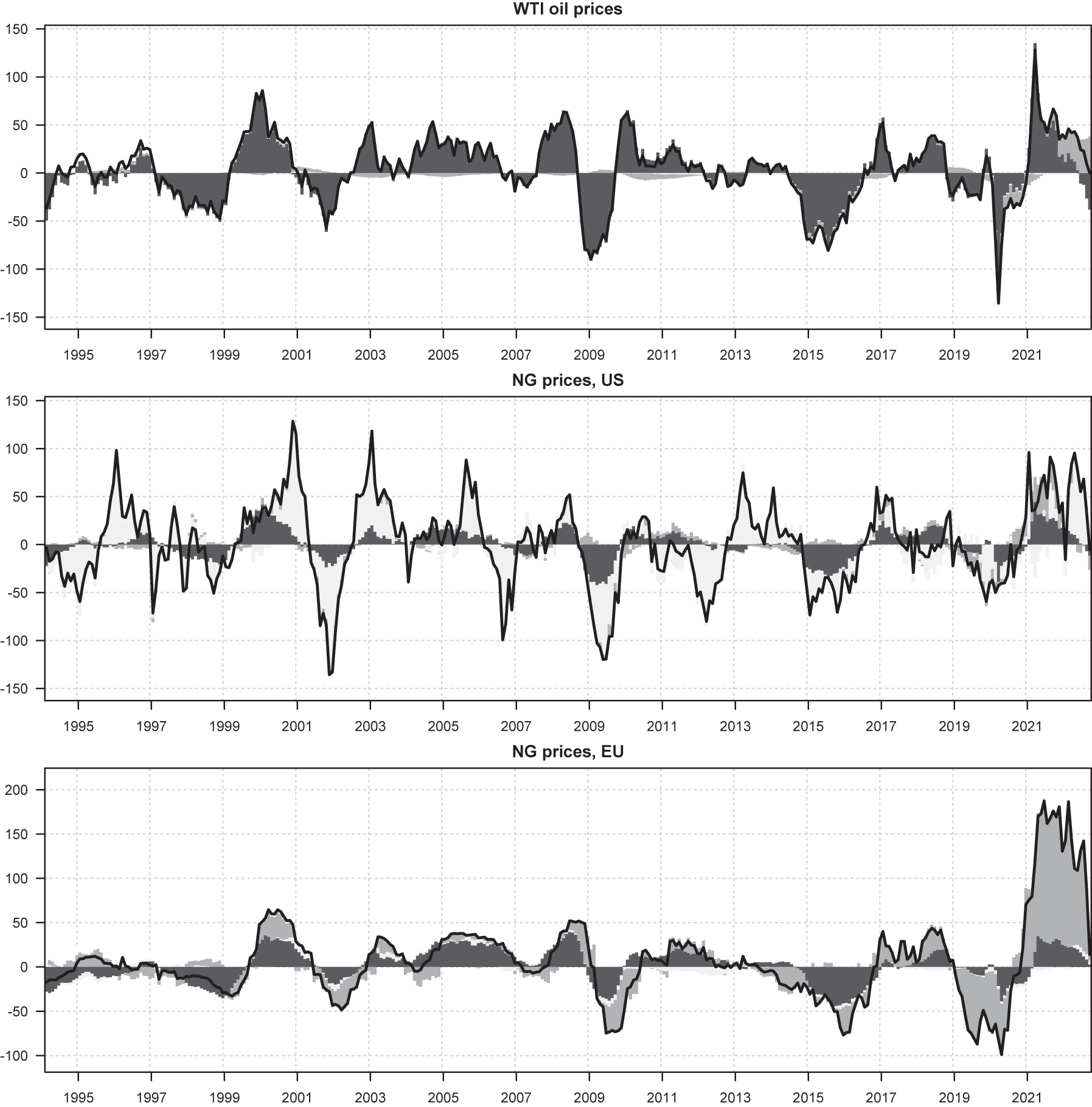
Historical decomposition for the log annual growth rate in real oil and natural gas prices in the constant coefficient SVAR model. The black solid line represents the logarithmic annual rate of change in the real prices of oil and natural gas (in per cent). The dark gray, light gray and medium gray colors represent the contribution of oil, US natural gas and EU natural gas market shocks (in pp), respectively.
3.3 Key takeaways
The above SVAR analysis allows us to make few observations. First, the comparison of IRFs for crude oil and US natural gas prices indicates that after the occurrence of η OIL and η NGUS innovations, both variables behave differently. This illustrates the observed decoupling of the US natural gas and crude oil markets. Second, the comparison of IRFs for crude oil and European natural gas prices indicates that after η OIL and η NGEU shocks there is only a temporary decoupling of both markets. However, after two years from the occurrence of shocks the reactions of both variables are almost the same. Moreover, after the η NGUS shock both variables behave similarly from the initial period onwards. This would indicate that the dynamics of these two markets are closely linked over medium and long-term horizons, but not over the short-term one. Next, the FEVD analysis shows that developments in the natural gas markets, both in the US and in Europe, affect crude oil prices only to a very limited extent. It also illustrates that US natural gas prices are not linked to oil prices neither in the short nor in the long horizon. Finally, FEVD confirms that European natural gas prices are linked to oil prices over the medium and long term. All the above results confirm findings presented in studies surveyed in Table 1, which do not account for the recent extreme market events. The new result of our SVAR analysis, which is driven by the most recent observations, is that at short-term horizon European natural gas market shocks significantly affect natural gas prices in the US as well as are exert an upward pressure on oil prices.
4 Time-varying parameters VAR approach
In the Introduction we have indicated that for the last decades the European natural gas market has undergone a structural change, including a gradual shift from oil price indexation to gas-on-gas pricing. Moreover, the results from the previous sections indicate that the developments in the European natural gas market in the last years were much different compared to the pre-Covid period. This would suggest that there are sound reasons to extend the structural VAR analysis by allowing for time-variation in model parameters and volatility of structural shocks.
In this section we employ the TVP-VAR-SV model proposed by Primiceri (2005) and subsequently refined by Del Negro and Primiceri (2015). We have decided to use this framework, rather than a regime-switching or threshold model, as it is considered to be best suited to describe the gradually evolving structure of the analyzed system, in our case the European natural gas market. Another reason for our choice is that this approach allows us to capture various sources of nonlinearities present in the system and pin down the varying magnitude of shocks, as all model parameters evolve continuously in time (Granger 2008; Lubik and Matthes 2015; Ng and Wright 2013). This feature should be of vital importance given the recent developments in the energy markets. The advantages of the TVP-VAR-SV model come at the cost of heavy parametrization and non-trivial estimation. Nonetheless, time-varying parameters models have become increasingly popular in various investigations, in particular related to the evolution and interplay of key macroeconomic variables (e.g. Anh et al. 2018; Bjørnland et al. 2019; Corsello and Nispi Landi 2020; Lubik et al. 2016; Primiceri 2005) or the developments in energy commodity markets (e.g. Anand and Paul 2021; Baumeister and Peersman 2013; Ding et al. 2021; Liu and Gong 2020; Lyu et al. 2021; Papiez et al. 2022; Shang and Hamori 2021; Wiggins and Etienne 2017).
4.1 The model
In the time-varying framework the dynamics of the dependent variable y t is given by a VAR process of order l = 2 according to the following rule of motion:
Note that now we allow all parameters, i.e. the vector of constant terms B
0,t
, the coefficients of the autoregressive matrices
To estimate the model efficiently we assume that
Given the above decomposition, we perform common VAR analysis in the time-varying framework by drawing from the posterior distribution. For that purpose we write down model (3) as:
where β
t
is a vector that collects all parameters from
Following Primiceri (2005), the time-varying parameters from vector β t and the free elements of matrix A t , which are stacked into α t = [a 21,t , a 31,t , a 32,t ]′, are governed by the standard random walk. In turn, the vector of standard deviations σ t = [σ 1t , σ 2t , σ 3t ]′ follows the geometric random walk. Consequently, they are specified as follows:
All innovations in the system are assumed to be mutually independent and normally distributed with the variance-covariance matrix:
where Q, S and W are positive definite, time-invariant matrices.
To estimate the model we rely on Bayesian methods, in particular the Markov Chain Monte Carlo (MCMC) approach and the Gibbs sampler proposed by Del Negro and Primiceri (2015). As regards the prior, we follow the procedure as well as choices described by Primiceri (2005), which is a standard approach in the literature (e.g. Anand and Paul 2021; Bjørnland et al. 2019; Chatziantoniou et al. 2021; Czudaj 2019; Lubik et al. 2016; Lyu et al. 2021). In the first step, we need to set the prior for the initial value of model parameters, i.e. β
0, α
0 and logσ
0. We do it by estimating the time-invariant VAR model of the form (1) using pre-sample observations. The point estimates (
As regards the hyperparameters specifying the tightness of the prior, we set them to the standard values from the literature, i.e. k β = 4, k α = 4, k σ = 1.
In the second step, we impose a prior on matrices Q, S and W by assuming that:
where
4.2 The results
The evolution of model parameters. We start our investigation of the TVP-VAR-SV model by inspecting the evolution of model parameters over time. The top and middle rows of Figure 5 present the posterior median for autoregressive coefficients along with the 90 % credible sets. The overwhelming impression is that for the baseline prior there is virtually no time variation for these parameters. On the contrary, the bottom row of the figure points to high variation in stochastic volatility parameters. It should be noted that this kind of outcome is typical for studies applying the TVP-VAR-SV framework (e.g. Anand and Paul 2021; Amir-Ahmadi et al. 2016; Cogley and Sargent 2005; Corsello and Nispi Landi 2020; Koop and Korobilis 2013; Lubik et al. 2016; Papiez et al. 2022; Primiceri 2005; Wiggins and Etienne 2017).

The evolution of selected coefficients in the TVP-VAR-SV model. The black solid line represents the posterior median, whereas the shaded area denotes the 90 percent posterior credible sets. The red line represent the posterior median in the model with hyperparameters k Q and k S multiplied and k W divided by a factor of 4.
The time-stability of the lag coefficients combined with large movements in stochastic volatility means that the propagation of shocks remains rather constant, whereas the strength of the impulse varies over time. In our case, there are several, occasional and short-lived increases in the time-varying standard deviation of shocks. The most pronounced spike in stochastic volatility occurred in the period following the outbreak of the Covid-19 pandemic, while smaller variation is also discernible during the global financial crisis. In the former case, this is especially visible for the European natural gas prices. Our reading of this result is that depending on the event, the initial reaction of energy commodity prices should differ, but their further development in time remains similar.
Impulse response functions. Given the evidence provided in Figure 5, we inspect market reaction during several specific time periods. These pertain to the:
Mar. 1996: cold winter in the US,
Dec. 2000: high US natural gas prices during the California crisis,
Sep. 2005: record high US natural gas prices due to the Katrina hurricane,
Jun. 2008: record high oil prices,
Feb. 2009: collapse in energy commodity prices during the global financial crisis (GFC),
Feb. 2014: cold winter in the US coupled with massive natural gas withdrawals,
Mar. 2018: the cold snap in Europe due to the impact of the “Beast from the East”,
Apr. 2020: most severe economic restrictions across the globe due to Covid-19,
Aug. 2022: record high European natural gas prices.
For all the above periods, in Figure 6 we present the posterior median impulse response. It illustrates that the propagation mechanism has indeed remained stable across the sample, while changes in IRFs originate mostly from the movements in stochastic volatility, i.e. the strength of the impulse. It can be seen that in seven episodes that occurred before 2020 the initial response of energy commodity prices is quite similar, despite different economic events. For instance, the top left panel illustrates that oil market shocks increase crude oil prices, with the standard magnitude of the response from around 7 % in winter 2014 to around 10 % throughout the deep recession during the GFC. However, most recently, following the outbreak of the Covid-19 pandemic, the reaction of oil prices to the oil shock almost doubled, amounting to over 15 % on impact and peaking at around 20 % shortly after the occurrence of shocks. The panel also shows that the pace of the return of oil prices to the pre-shock level remained broadly the same, with half-life amounting to about 5 years, in line with the literature on real commodity price persistence (e.g. Ghoshray et al. 2014; Rubaszek 2021). The remaining two top panels of the figure show that the sensitivity of oil prices to natural gas market shocks in the US and in Europe is limited. Again, we observe two grouped sets of IRFs, before and during Covid-19. Interestingly, the peak of the impact of the US natural gas market shock on oil prices realizes far later after the occurrence of the shock than in the case of the EU shock.

Impulse response functions in the TVP-VAR-SV model. The solid lines represent the posterior median impulse responses at various points in time. Market events are described in Section 4.2. All values are multiplied by 100 so that they are expressed as per cents.
The middle row of Figure 6 describes the reaction of US natural gas prices to the three structural shocks. In the first year after the oil price shock the reaction of US natural gas prices varies from around 4 % to almost 9 %. It can be noticed that the pace of reversion is considerably slower than in the constant coefficient VAR. The center panel shows that during most recent events US natural gas prices reaction to market-specific shock amounted to as much as 20 %, visibly more than during the cold winter of 1996, the California crisis, the Hurricane Katrina episode or the record withdrawals in 2014.
The bottom row of Figure 6 illustrates how the reaction of European natural gas prices to the structural shocks evolves over time. Following oil shocks there is a sizable, although lagged, response of EU natural gas prices. The peak response takes place around two years after the shock and is estimated to amount between 6 % and 14 %, depending on the episode. The central panel shows that the situation on the US natural gas market does not influence EU prices in a significant way, leading to the decoupling of gas prices across the Atlantic. Instead, EU market specific shocks tend to significantly impact European natural gas prices, with the response amounting even to around 23 % for selected episodes and horizons. It should be emphasized that in this case the pace of reversion to pre-shock level is relatively quick, with half-life of about one year.
A careful look at Figure 6 leads to the observation that at longer horizons the responses of oil and European natural gas prices to all shocks are almost the same, which is not the case for shorter horizons. In the case of the oil shock, this is illustrated in detail in Figure 7. Specifically, it presents the ratio of oil to European natural gas price response, at various horizons and for different moments in time, so that a value of 1 means that the reactions of both variables are the same. The figure delivers strong evidence that the decoupling of European natural gas prices from oil prices is short-lived. At horizons above 2 years, the reaction of both variables is almost exactly the same, without any restrictions imposed on VAR model parameters. Moreover, this result is valid across the sample, which covers almost three last decades.

The short-term divergence and long-term convergence of oil and EU natural gas prices. Each bar represents the ratio of the median reaction of oil prices and EU natural gas prices to the oil shock at a specific horizon and for a certain market event. A value of one means that the change in prices of both commodities is the same.
We continue our investigation by checking how the use of the TVP-VAR-SV framework influences our perception about the dynamics of the analyzed trivariate system for energy commodity prices compared to the broadly used constant coefficient structural VAR model. In Figure 8 we compare posterior median IRF obtained from the TVP-VAR-SV approach for the last period of the sample to the IRF obtained from the structural VAR. This allows us to study how both models behave if estimated using information available at the end of our sample. In general, we observe that in the TVP-VAR-SV model the response of energy commodity prices to shocks is more pronounced and sometimes more persistent than in the structural VAR model. However, both models are unanimously pointing to the segmentation of gas markets and to the link between European natural gas and crude oil prices in the longer horizons. This would suggest that, despite the changes in the structure of the European natural gas market, including a shift from the oil price indexation towards gas-on gas competition, European prices are still linked to oil prices over the long-term horizon.

The comparison of impulse response functions in the SVAR and TVP-VAR-SV model. The black solid line represents the posterior median, whereas the shaded area denotes the 90 percent posterior credible sets for the last period in the sample from the time-varying parameters SVAR model (i.e. October 2022). The dashed line illustrates the impulse response function from the constant coefficient SVAR model. All values are multiplied by 100 so that they are expressed as per cents.
Forecast error variance decomposition. We conclude the TVP-VAR-SV analysis by quantifying time-varying contribution of the three shocks to the forecast error variance of endogenous variables at four selected horizons, i.e. on impact, after one year, three years and five years ahead. The top row of Figure 9 shows that in the very short-term energy commodities prices are almost exclusively driven by market-specific shocks. The left column of the figure indicates that for oil prices the contribution of idiosyncratic shock to variance remains dominant also at longer horizons. Specifically, in the long run around 90 % of their variability stems from the shock specific to the oil market, while the contribution of US and EU natural gas market shocks are negligible. As regards natural gas prices, we observe sizeable discrepancies between the US and EU markets. For the former, the role of idiosyncratic shocks is dominant for all horizons and periods. The contribution of oil and European gas market shocks is usually below 25 % and 5 %, respectively. In the case of European natural gas prices the situation is different. The contribution of oil market shocks to forecast error variance at the five-year horizon stands approximately at 80 % throughout the majority of the sample, which points to the strong link between both energy commodity prices over the long-run. However, the figure also shows that there has been a gradual increase in the contribution of idiosyncratic shocks to the forecast error variance to around 33 % at the end of the sample, which might reflect the changing structure of the European natural gas market. Finally, it can be seen that the developments in the US natural gas market play a minor role in the evolution of EU natural gas prices.
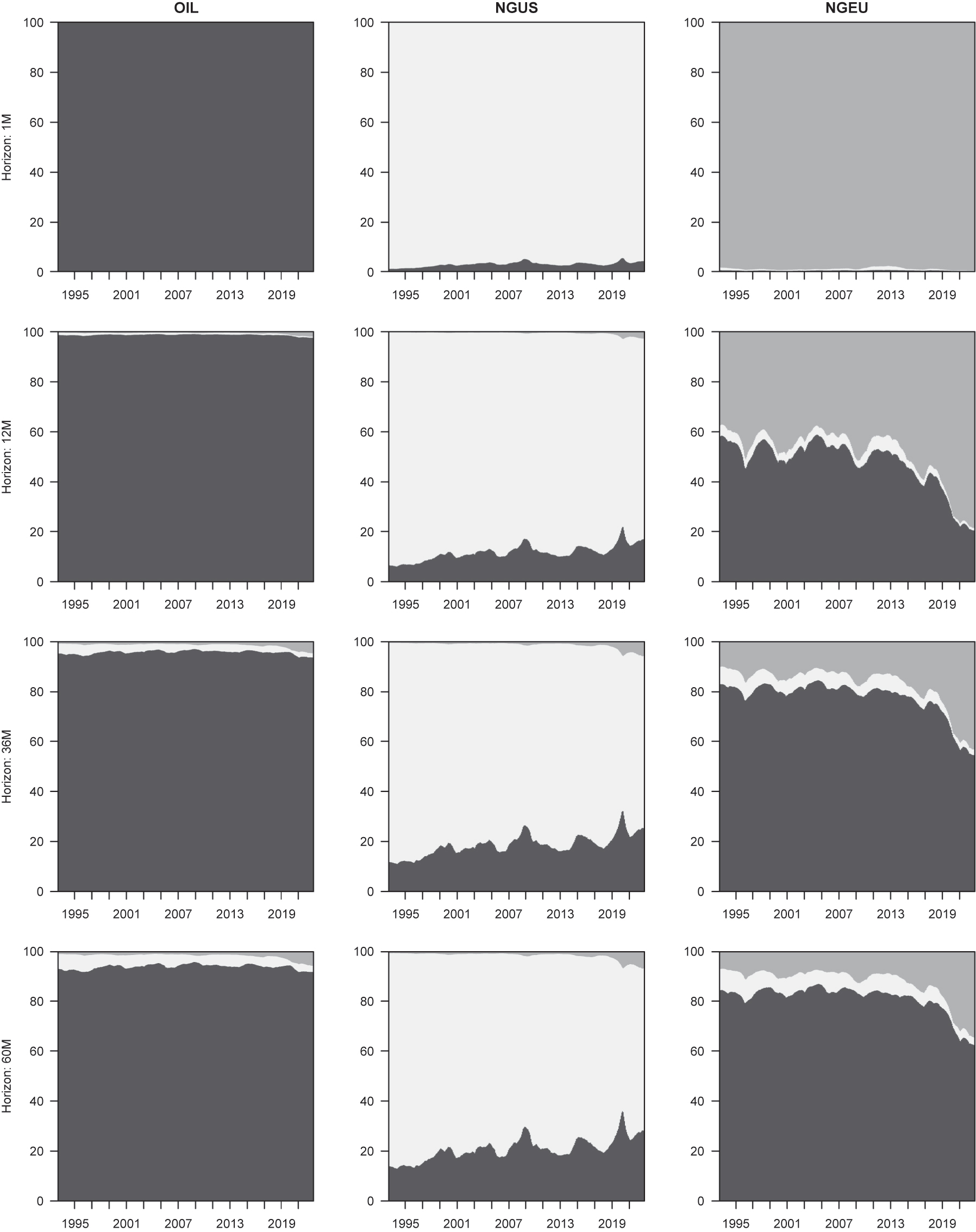
Forecast error variance decomposition in the TVP-VAR-SV model. The figure presents the evolution of the forecast error variance decomposition for the log level in real oil and natural gas prices. The dark gray, light gray and medium gray colors represent the contribution of oil, US natural gas and EU natural gas markets shocks (in per cents), respectively. As median contributions are reported, their sum is normalized to add up to 100.
4.3 Sensitivity analysis
In the baseline specification of the prior for the TVP-VAR-SV model we fix hyperparameters k Q , k S and k W at values most commonly used in the literature. As a robustness check, we rescale them by a factor of 4, so that k Q = 0.04, k W = 0.0025 and k S = 0.40. This modification introduces more freedom in the evolution of autoregressive parameters and, at the same time, constrains changes in stochastic volatility components.
The impact of this change on the posterior median of model parameters is hardly visible, which is illustrated in Figure 5. Rescaling the prior has very small effect on the shape of impulse-response functions (Figure 10) and forecast error variance decomposition (Figure 11). Thus, we conclude that our results are robust to reasonable changes in prior assumptions.

IRF in the TVP-VAR-SV model with hyperparameters rescaled by 4. The solid lines represent the posterior median impulse responses at various points in time from the model with hyperparameters k Q and k S multiplied and k W divided by a factor of 4. Market events are described in Section 4.2. All values are multiplied by 100 so that they are expressed as per cents.

FEVD in the TVP-VAR-SV model with hyperparameters rescaled by 4. The figure presents the evolution of the forecast error variance decomposition for the log level in real oil and natural gas prices based on the model with hyperparameters k Q and k S multiplied and k W divided by a factor of 4. The dark gray, light gray and medium gray colors represent the contribution of oil, US natural gas and EU natural gas markets shocks (in per cents), respectively. As median contributions are reported, their sum is normalized to add up to 100.
4.4 Key takeaways
The TVP-VAR analysis allows us to infer the following. An important new result of our investigation is that on energy commodity markets shocks propagation mechanism is stable, whereas the strength of structural impulses turned out to be volatile. In particular, we observe its multi-fold increase throughout the Covid-19 pandemic and since the onset of the Russian invasion of Ukraine. Secondly, we have delivered updated evidence to the literature surveyed in Table 1 by showing that even despite recent extreme market events the decoupling of European natural gas prices from oil prices remains short-lived as there exists a long-term link of both commodities at horizons above 2 years. It should be emphasized that this result, which is stable throughout the entire sample, was derived using unrestricted VAR model. Finally, using a very flexible estimation framework, in this section we have confirmed previous evidence on low sensitivity of oil prices to natural gas market shocks as well as the decoupling of gas prices across the Atlantic.
5 Conclusion and discussion
In this article we have investigated the joint dynamics of crude oil and natural gas prices in the US and Europe over the years 1993–2022. Our aim was to establish the relationship among the three analyzed variables and assess how this relationship evolves over time. The main research question was if prices of these energy commodities are determined together or rather evolve independently. For that purpose we have developed and simulated constant and time-varying parameters structural VAR models.
Our results confirm and extend two previous findings from the literature. Specifically, we have found that fluctuations of oil prices to a very limited extent are affected by shocks specific to natural gas markets, whether American or European. Second, we have shown that the dynamics of the US natural gas market is predominantly driven by idiosyncratic innovations and is only partially affected by crude oil shocks. In other words, we confirm that after deregulation US natural gas prices and crude oil prices have separated from each other. However, by using data covering Covid-19 period and the Russian invasion of Ukraine, we have identified a significant short-term reaction of US natural gas prices to European natural gas market disturbance.
What is most important, we have presented new insights about the functioning of the European natural gas market. For the last three decades it has undergone a profound transformation, including the deregulation process and a shift from oil price indexation towards gas-on-gas competition. It can be therefore expected that, similarly to what has been observed in the US, natural gas prices should decouple from oil prices and be fully determined by market-specific forces. This kind of expectations could have been recently reinforced by unprecedented spikes in European natural gas prices, which strongly exceeded increases in crude oil prices. Indeed, since October 2021 the price of natural gas in Europe was much higher than the price of crude oil, if both expressed in the same energy unit (recall Figure 1). Our results are not supporting this decoupling story. They indicate that over longer horizons European natural gas prices remain strongly linked to oil prices. The structural VAR analysis shows that decoupling of both variables is short-lived, whereas simulations with the TVP-VAR-SV model demonstrate that this kind of dependence among both variables is stable over the investigated period.
One might therefore ask why the deregulation process has not broken the link between natural gas and crude oil prices in Europe, as it happened in the US. One of the reasons might be that Europe has not experienced shale gas revolution. In the US, it has led to oversupply of natural gas that, due to the lack of infrastructure, could not be easily exported. The second reason is that unlike in the US, the supply of natural gas in Europe is predominantly based on imports through pipelines from conventional sources. Even within gas-on-gas competition, natural gas exporters might decide to limit supply if prices are too low compared to oil prices as they implicitly apply oil indexation. In this respect, the price elasticity of natural gas supply from Russia, Algeria and Norway to the European market is worthy of a detailed investigation.
Our second important new result is that the impact of the shale gas revolution, originating in the US, on the European natural gas market has been so far hardly visible. Again, one can expect that the development of LNG infrastructure, hence increased linkages of the US and European natural gas markets, should enable the arbitrage across the Atlantic and the elimination of the substantial price gap observed after the shale gas revolution in the US. So far this arbitrage has not worked due to the lack of liquefying capacities in the US. In consequence, natural gas prices in both markets evolve almost independently. However, with the further development of the infrastructure, which has recently seriously accelerated as a result of Europe’s effort to become independent of Russia’s natural gas supply,[2] European countries might have a better bargaining position in negotiating new contracts for imports. This factor can help in the shift of the European natural gas market from crude oil pricing into pricing based on market forces determined by current supply and demand. At the same time, higher exports capacities of LNG in the US might also weaken the divergence of the US gas market from the crude oil market.
The limitation of our study is that we have not considered a broader set of fundamentals, which affect European natural gas prices. In fact, all local factors are in our study represented by a single “EU natural gas prices” shock. This calls for future research aimed at distinguishing economic and financial drivers of natural gas market dynamics in Europe. One direction would be to build an empirical model of richer specification, similarly to what was done for the US gas market by Wiggins and Etienne (2017) or Rubaszek et al. (2021). The other direction would be to elaborate a theoretical model describing the functioning of the European natural gas market, similarly what was done for the global crude oil market by Nakov and Pescatori (2010). This kind of investigations would be helpful to better understand the sources of natural price dynamics in Europe.
Having in mind the above limitation, we believe that our findings help in better understanding the evolving joint dynamics of the three energy commodity prices. The results of our analysis contain new insights important in designing and developing the common European natural gas policy. An important policy implication of our study comes from the notion that expecting the decoupling of EU natural gas prices from crude oil prices along the deregulation process of the European gas market might be premature. Indeed, we have confirmed the existence of the long-term link between European natural gas and crude oil prices. Consequently, it might be claimed that the reform of natural gas market in Europe, which was largely replicating the deregulation process in the US, has not delivered expected results. Even though it has substituted oil price indexation by gas-on-gas pricing, it has not resulted in decoupling of natural gas from crude oil prices. The other interesting observation based the developments over the period of Russian invasion of Ukraine is that price elasticity of natural gas supply in Europe is relatively low, which can be justified by its geographical structure. This leads to extremely high natural gas price response to supply shocks, usually originating outside EU, and puts into question if natural gas prices should be determined solely by market forces. Finally, the implication of our study related to the most recent spikes in European natural gas prices is clear: they should be short-lived. In technical terms, the TVP-VAR-SV model interprets these spikes as the realization of highly volatile idiosyncratic shocks, rather than decoupling of natural gas and oil markets. As a result, we should expect gradual reversion of European natural gas prices to the equilibrium value given by oil prices.
Funding source: Narodowe Centrum Nauki
Award Identifier / Grant number: 2020/39/B/HS4/00366
Acknowledgements
We are grateful for comments from the SNDE Editor, prof. Bruce Mizrach, an anonymous Reviewer, our discussant at the FMND 2022 conference, Elena Maria Diaz. We also thank for the feedback from the participants of FMND 2022 (Paris 2022) and Summer Workshop in Macroeconomics and Finance (Warsaw 2022) conferences.
-
Author contributions: All the authors have accepted responsibility for the entire content of this submitted manuscript and approved submission.
-
Research funding: This article was realized thanks to the financial support from the National Science Centre (Poland) within grant No. 2020/39/B/HS4/00366.
-
Conflict of interest statement: The authors declare no conflicts of interest regarding this article.
References
Amir-Ahmadi, P., C. Matthes, and M.-C. Wang. 2016. “Drifts and Volatilities under Measurement Error: Assessing Monetary Policy Shocks over the Last Century.” Quantitative Economics 7: 591–611. https://doi.org/10.3982/qe475.Search in Google Scholar
Anand, B., and S. Paul. 2021. “Oil Shocks and Stock Market: Revisiting the Dynamics.” Energy Economics 96: 105111. https://doi.org/10.1016/j.eneco.2021.105111.Search in Google Scholar
Anh, N., E. Pavlidis, and D. Peel. 2018. “Modeling Changes in US Monetary Policy with a Time-Varying Nonlinear Taylor Rule.” Studies in Nonlinear Dynamics & Econometrics 22: 1–17.10.1515/snde-2017-0092Search in Google Scholar
Arora, V., and J. Lieskovsky. 2014. “Natural Gas and U.S. Economic Activity.” Energy Journal 35: 167–82. https://doi.org/10.5547/01956574.35.4.8.Search in Google Scholar
Asche, F., A. Oglend, and P. Osmundsen. 2017. “Modeling UK Natural Gas Prices when Gas Prices Periodically Decouple from the Oil Price.” Energy Journal 38: 131–48. https://doi.org/10.5547/01956574.38.2.fasc.Search in Google Scholar
Bastianin, A., M. Galeotti, and M. Polo. 2019. “Convergence of European Natural Gas Prices.” Energy Economics 81: 793–811. https://doi.org/10.1016/j.eneco.2019.05.017.Search in Google Scholar
Batten, J. A., C. Ciner, and B. M. Lucey. 2017. “The Dynamic Linkages between Crude Oil and Natural Gas Markets.” Energy Economics 62: 155–70. https://doi.org/10.1016/j.eneco.2016.10.019.Search in Google Scholar
Baumeister, C., and G. Peersman. 2013. “Time-varying Effects of Oil Supply Shocks on the US Economy.” American Economic Journal: Macroeconomics 5: 1–28. https://doi.org/10.1257/mac.5.4.1.Search in Google Scholar
Bjørnland, H. C., L. A. Thorsrud, and R. Torvik. 2019. “Dutch Disease Dynamics Reconsidered.” European Economic Review 119: 411–33. https://doi.org/10.1016/j.euroecorev.2019.07.016.Search in Google Scholar
Bouwmeester, M. C., and J. Oosterhaven. 2017. “Economic Impacts of Natural Gas Flow Disruptions between Russia and the EU.” Energy Policy 106: 288–97. https://doi.org/10.1016/j.enpol.2017.03.030.Search in Google Scholar
Broadstock, D. C., R. Li, and L. Wang. 2020. “Integration Reforms in the European Natural Gas Market: A Rolling-Window Spillover Analysis.” Energy Economics 92: 104939. https://doi.org/10.1016/j.eneco.2020.104939.Search in Google Scholar
Brown, S., and M. Yucel. 2009. “Market Arbitrage: European and North American Natural Gas Prices.” Energy Journal 30: 167–86. https://doi.org/10.5547/issn0195-6574-ej-vol30-nosi-11.Search in Google Scholar
Chatziantoniou, I., M. Filippidis, G. Filis, and D. Gabauer. 2021. “A Closer Look into the Global Determinants of Oil Price Volatility.” Energy Economics 95: 105092. https://doi.org/10.1016/j.eneco.2020.105092.Search in Google Scholar
Chyong, C. K. 2019. “European Natural Gas Markets: Taking Stock and Looking Forward.” Review of Industrial Organization 55: 89–109. https://doi.org/10.1007/s11151-019-09697-3.Search in Google Scholar
Cogley, T., and T. J. Sargent. 2005. “Drifts and Volatilities: Monetary Policies and Outcomes in the Post WWII US.” Review of Economic Dynamics 8: 262–302. https://doi.org/10.1016/j.red.2004.10.009.Search in Google Scholar
Corsello, F., and V. Nispi Landi. 2020. “Labor Market and Financial Shocks: A Time-Varying Analysis.” Journal of Money, Credit, and Banking 52: 777–801. https://doi.org/10.1111/jmcb.12638.Search in Google Scholar
Czudaj, R. L.. 2019. “Crude Oil Futures Trading and Uncertainty.” Energy Economics 80: 793–811. https://doi.org/10.1016/j.eneco.2019.01.002.Search in Google Scholar
Del Negro, M., and G. E. Primiceri. 2015. “Time Varying Structural Vector Autoregressions and Monetary Policy: A Corrigendum.” The Review of Economic Studies 82: 1342–5. https://doi.org/10.1093/restud/rdv024.Search in Google Scholar
del Valle, A., P. Dueñas, S. Wogrin, and J. Reneses. 2017. “A Fundamental Analysis on the Implementation and Development of Virtual Natural Gas Hubs.” Energy Economics 67: 520–32. https://doi.org/10.1016/j.eneco.2017.08.001.Search in Google Scholar
Ding, Q., J. Huang, and H. Zhang. 2021. “The Time-Varying Effects of Financial and Geopolitical Uncertainties on Commodity Market Dynamics: A TVP-SVAR-SV Analysis.” Resources Policy 72: 102079. https://doi.org/10.1016/j.resourpol.2021.102079.Search in Google Scholar
Erdos, P.. 2012. “Have Oil and Gas Prices Got Separated?” Energy Policy 49: 707–18. https://doi.org/10.1016/j.enpol.2012.07.022.Search in Google Scholar
Gao, S., C. Hou, and B. H. Nguyen. 2021. “Forecasting Natural Gas Prices Using Highly Flexible Time-Varying Parameter Models.” Economic Modelling 105:105652. https://doi.org/10.1016/j.econmod.2021.105652.Search in Google Scholar
Geng, J.-B., Q. Ji, and Y. Fan. 2016a. “How Regional Natural Gas Markets Have Reacted to Oil Price Shocks before and since the Shale Gas Revolution: A Multi-Scale Perspective.” Journal of Natural Gas Science and Engineering 36: 734–46. https://doi.org/10.1016/j.jngse.2016.11.020.Search in Google Scholar
Geng, J.-B., Q. Ji, and Y. Fan. 2016b. “The Impact of the North American Shale Gas Revolution on Regional Natural Gas Markets: Evidence from the Regime-Switching Model.” Energy Policy 96: 167–78. https://doi.org/10.1016/j.enpol.2016.05.047.Search in Google Scholar
Ghoshray, A., M. Kejriwal, and M. Wohar. 2014. “Breaks, Trends and Unit Roots in Commodity Prices: A Robust Investigation.” Studies in Nonlinear Dynamics & Econometrics 18: 23–40. https://doi.org/10.1515/snde-2013-0022.Search in Google Scholar
Gong, X., Y. Liu, and X. Wang. 2021. “Dynamic Volatility Spillovers across Oil and Natural Gas Futures Markets Based on a Time-Varying Spillover Method.” International Review of Financial Analysis 76: 101790. https://doi.org/10.1016/j.irfa.2021.101790.Search in Google Scholar
Granger, C. 2008. “Non-Linear Models: Where Do We Go Next - Time Varying Parameter Models?” Studies in Nonlinear Dynamics & Econometrics 12: 1–11. https://doi.org/10.2202/1558-3708.1639.Search in Google Scholar
Hailemariam, A., and R. Smyth. 2019. “What Drives Volatility in Natural Gas Prices?” Energy Economics 80: 731–42. https://doi.org/10.1016/j.eneco.2019.02.011.Search in Google Scholar
Hou, C., and B. H. Nguyen. 2018. “Understanding the US Natural Gas Market: A Markov Switching VAR Approach.” Energy Economics 75: 42–53. https://doi.org/10.1016/j.eneco.2018.08.004.Search in Google Scholar
Hulshof, D., J.-P. van der Maat, and M. Mulder. 2016. “Market Fundamentals, Competition and Natural-Gas Prices.” Energy Policy 94: 480–91. https://doi.org/10.1016/j.enpol.2015.12.016.Search in Google Scholar
IEA. 2021. Oil Market Report. International Energy Agency.Search in Google Scholar
IGU. 2021. Wholesale Gas Price Survey. Barcelona: International Gas Union.Search in Google Scholar
Jadidzadeh, A., and A. Serletis. 2017. “How Does the U.S. Natural Gas Market React to Demand and Supply Shocks in the Crude Oil Market?” Energy Economics 63: 66–74. https://doi.org/10.1016/j.eneco.2017.01.007.Search in Google Scholar
Ji, Q., J.-B. Geng, and A. K. Tiwari. 2018. “Information Spillovers and Connectedness Networks in the Oil and Gas Markets.” Energy Economics 75: 71–84. https://doi.org/10.1016/j.eneco.2018.08.013.Search in Google Scholar
Joskow, P. L.. 2013. “Natural Gas: From Shortages to Abundance in the United States.” The American Economic Review 103: 338–43. https://doi.org/10.1257/aer.103.3.338.Search in Google Scholar
Kan, S., B. Chen, X. Wu, Z. Chen, and G. Chen. 2019. “Natural Gas Overview for World Economy: From Primary Supply to Final Demand via Global Supply Chains.” Energy Policy 124: 215–25. https://doi.org/10.1016/j.enpol.2018.10.002.Search in Google Scholar
Kilian, L. 2009. “Not All Oil Price Shocks Are Alike: Disentangling Demand and Supply Shocks in the Crude Oil Market.” The American Economic Review 99: 1053–69. https://doi.org/10.1257/aer.99.3.1053.Search in Google Scholar
Koop, G., and D. Korobilis. 2013. “Large Time-Varying Parameter VARs.” Journal of Econometrics 177: 185–98. https://doi.org/10.1016/j.jeconom.2013.04.007.Search in Google Scholar
Lin, B., and J. Li. 2015. “The Spillover Effects across Natural Gas and Oil Markets: Based on the VEC-MGARCH Framework.” Applied Energy 155: 229–41. https://doi.org/10.1016/j.apenergy.2015.05.123.Search in Google Scholar
Liu, T., and X. Gong. 2020. “Analyzing Time-Varying Volatility Spillovers between the Crude Oil Markets Using a New Method.” Energy Economics 87: 104711. https://doi.org/10.1016/j.eneco.2020.104711.Search in Google Scholar
Lubik, T. A., and C. Matthes. 2015. “Time-varying Parameter Vector Autoregressions: Specification, Estimation, and an Application.” Economic Quarterly 101 (4): 323–52, https://doi.org/10.21144/eq1010403.Search in Google Scholar
Lubik, T. A., C. Matthes, and A. Owens. 2016. “Beveridge Curve Shifts and Time-Varying Parameter VARs.” Economic Quarterly 102 (3): 197–226, https://doi.org/10.21144/eq1020302.Search in Google Scholar
Lyu, Y., S. Tuo, Y. Wei, and M. Yang. 2021. “Time-varying Effects of Global Economic Policy Uncertainty Shocks on Crude Oil Price Volatility: New Evidence.” Resources Policy 70: 101943. https://doi.org/10.1016/j.resourpol.2020.101943.Search in Google Scholar
Mu, X., and H. Ye. 2018. “Towards an Integrated Spot LNG Market: An Interim Assessment.” Energy Journal 39: 211–34. https://doi.org/10.5547/01956574.39.1.xmu.Search in Google Scholar
Nakov, A., and A. Pescatori. 2010. “Oil and the Great Moderation.” The Economic Journal 120: 131–55. https://doi.org/10.1111/j.1468-0297.2009.02302.x.Search in Google Scholar
Ng, S., and J. H. Wright. 2013. “Facts and Challenges from the Great Recession for Forecasting and Macroeconomic Modeling.” Journal of Economic Literature 51: 1120–54. https://doi.org/10.1257/jel.51.4.1120.Search in Google Scholar
Nguyen, B. H., and T. Okimoto. 2019. “Asymmetric Reactions of the US Natural Gas Market and Economic Activity.” Energy Economics 80: 86–99. https://doi.org/10.1016/j.eneco.2018.12.015.Search in Google Scholar
Nick, S., and S. Thoenes. 2014. “What Drives Natural Gas Prices? A Structural VAR Approach.” Energy Economics 45: 517–27. https://doi.org/10.1016/j.eneco.2014.08.010.Search in Google Scholar
Papiez, M., M. Rubaszek, K. Szafranek, and S. Smiech. 2022. “Are European Natural Gas Markets Connected? a Time-Varying Spillovers Analysis.” Resources Policy 79: 103029. https://doi.org/10.1016/j.resourpol.2022.103029.Search in Google Scholar
Primiceri, G. E. 2005. “Time Varying Structural Vector Autoregressions and Monetary Policy.” The Review of Economic Studies 72: 821–52. https://doi.org/10.1111/j.1467-937x.2005.00353.x.Search in Google Scholar
Rodriguez-Gomez, N., N. Zaccarelli, and R. Bolado-Lavín. 2016. “European Ability to Cope with a Gas Crisis. Comparison between 2009 and 2014.” Energy Policy 97: 461–74. https://doi.org/10.1016/j.enpol.2016.07.016.Search in Google Scholar
Rubaszek, M. 2021. “Forecasting Crude Oil Prices with DSGE Models.” International Journal of Forecasting 37: 531–46. https://doi.org/10.1016/j.ijforecast.2020.07.004.Search in Google Scholar
Rubaszek, M., Z. Karolak, M. Kwas, and G. S. Uddin. 2020. “The Role of the Threshold Effect for the Dynamics of Futures and Spot Prices of Energy Commodities.” Studies in Nonlinear Dynamics & Econometrics 24: 1–20. https://doi.org/10.1515/snde-2019-0068.Search in Google Scholar
Rubaszek, M., and G. S. Uddin. 2020. “The Role of Underground Storage in the Dynamics of the US Natural Gas Market: A Threshold Model Analysis.” Energy Economics 87: 104713. https://doi.org/10.1016/j.eneco.2020.104713.Search in Google Scholar
Rubaszek, M., G. S. Uddin, and K. Szafranek. 2021. “The Dynamics and Elasticities on the U.S. Natural Gas Market. A Bayesian Structural VAR Analysis.” Energy Economics 103: 105526. https://doi.org/10.1016/j.eneco.2021.105526.Search in Google Scholar
Shang, J., and S. Hamori. 2021. “Do Crude Oil Prices and the Sentiment Index Influence Foreign Exchange Rates Differently in Oil-Importing and Oil-Exporting Countries? A Dynamic Connectedness Analysis.” Resources Policy 74: 102400. https://doi.org/10.1016/j.resourpol.2021.102400.Search in Google Scholar
Siliverstovs, B., G. L’Hegaret, A. Neumann, and C. von Hirschhausen. 2005. “International Market Integration for Natural Gas? a Cointegration Analysis of Prices in Europe, North america and japan.” Energy Economics 27: 603–15. https://doi.org/10.1016/j.eneco.2005.03.002.Search in Google Scholar
Stern, J.. 2014. “International Gas Pricing in Europe and Asia: A Crisis of Fundamentals.” Energy Policy 64: 43–8. https://doi.org/10.1016/j.enpol.2013.05.127.Search in Google Scholar
Tiwari, A. K., Z. Mukherjee, R. Gupta, and M. Balcilar. 2019. “A Wavelet Analysis of the Relationship between Oil and Natural Gas Prices.” Resources Policy 60: 118–24. https://doi.org/10.1016/j.resourpol.2018.11.020.Search in Google Scholar
Wakamatsu, H., and K. Aruga. 2013. “The Impact of the Shale Gas Revolution on the U.S. And Japanese Natural Gas Markets.” Energy Policy 62: 1002–9. https://doi.org/10.1016/j.enpol.2013.07.122.Search in Google Scholar
Wiggins, S., and X. L. Etienne. 2017. “Turbulent Times: Uncovering the Origins of US Natural Gas Price Fluctuations since Deregulation.” Energy Economics 64: 196–205. https://doi.org/10.1016/j.eneco.2017.03.015.Search in Google Scholar
Zhang, D., and Q. Ji. 2018. “Further Evidence on the Debate of Oil-Gas Price Decoupling: A Long Memory Approach.” Energy Policy 113: 68–75. https://doi.org/10.1016/j.enpol.2017.10.046.Search in Google Scholar
Supplementary Material
This article contains supplementary material (https://doi.org/10.1515/snde-2022-0051).
© 2023 the author(s), published by De Gruyter, Berlin/Boston
This work is licensed under the Creative Commons Attribution 4.0 International License.
Articles in the same Issue
- Frontmatter
- Research Articles
- Welfare cost of inflation, when credit card transaction services are included among monetary services
- Co-Jumping of Treasury Yield Curve Rates
- Have European natural gas prices decoupled from crude oil prices? Evidence from TVP-VAR analysis
- Stability in Threshold VAR Models
- Examining the Impact of Energy Policies on CO2 Emissions with Information and Communication Technologies and Renewable Energy
- Interfuel Substitution and Inflation Dynamics in India