Estimation of long memory in volatility using wavelets
-
Lucie Kraicová


Abstract
This work studies wavelet-based Whittle estimator of the fractionally integrated exponential generalized autoregressive conditional heteroscedasticity (FIEGARCH) model often used for modeling long memory in volatility of financial assets. The newly proposed estimator approximates the spectral density using wavelet transform, which makes it more robust to certain types of irregularities in data. Based on an extensive Monte Carlo study, both behavior of the proposed estimator and its relative performance with respect to traditional estimators are assessed. In addition, we study properties of the estimators in presence of jumps, which brings interesting discussion. We find that wavelet-based estimator may become an attractive robust and fast alternative to the traditional methods of estimation. In particular, a localized version of our estimator becomes attractive in small samples.
Acknowledgments
We would like to express our gratitude to Ana Perez, who provided us with the code for MLE and FWE estimation of FIEGARCH processes, and we gratefully acknowledge financial support from the the Czech Science Foundation under project No. 13-32263S. The research leading to these results has received funding from the European Unions Seventh Framework Programme (FP7/2007-2013) under grant agreement No. FP7-SSH- 612955 (FinMaP).
A Appendix: Tables and Figures
Energy decomposition.
| Coefficients | d | ω | α | β | θ | γ |
|---|---|---|---|---|---|---|
| (a) Coefficient sets | ||||||
| A | 0.25 | 0 | 0.5 | 0.5 | −0.3 | 0.5 |
| B | 0.45 | 0 | 0.5 | 0.5 | −0.3 | 0.5 |
| C | −0.25 | 0 | 0.5 | 0.5 | −0.3 | 0.5 |
| D | 0.25 | 0 | 0.9 | 0.9 | −0.3 | 0.5 |
| E | 0.45 | 0 | 0.9 | 0.9 | −0.3 | 0.5 |
| F | −0.25 | 0 | 0.9 | 0.9 | −0.3 | 0.5 |
| G | 0.25 | 0 | 0.9 | 0.9 | −0.9 | 0.9 |
| H | 0.45 | 0 | 0.9 | 0.9 | −0.9 | 0.9 |
| A | B | C | D | E | F | G | H | |
|---|---|---|---|---|---|---|---|---|
| (b) Integrals over frequencies respective to levels for the coefficient sets from Table 1 | ||||||||
| Level 1 | 1.1117 | 1.1220 | 1.0897 | 1.1505 | 1.1622 | 1.1207 | 1.1261 | 1.1399 |
| Level 2 | 0.5473 | 0.5219 | 0.6274 | 0.4776 | 0.4691 | 0.5306 | 0.6187 | 0.6058 |
| Level 3 | 0.3956 | 0.3693 | 0.4330 | 0.3246 | 0.3056 | 0.3959 | 1.1354 | 1.3453 |
| Level 4 | 0.3029 | 0.3341 | 0.2425 | 0.5559 | 0.7712 | 0.3528 | 2.9558 | 4.8197 |
| Level 5 | 0.2035 | 0.2828 | 0.1175 | 1.0905 | 2.1758 | 0.3003 | 6.0839 | 13.2127 |
| Level 6 | 0.1279 | 0.2297 | 0.0550 | 1.4685 | 3.9342 | 0.1965 | 8.2136 | 23.4144 |
| Level 7 | 0.0793 | 0.1883 | 0.0259 | 1.3523 | 4.7975 | 0.0961 | 7.6026 | 28.4723 |
| Level 8 | 0.0495 | 0.1584 | 0.0123 | 1.0274 | 4.8302 | 0.0408 | 5.8268 | 28.7771 |
| Level 9 | 0.0313 | 0.1368 | 0.0059 | 0.7327 | 4.5720 | 0.0169 | 4.1967 | 27.3822 |
| Level 10 | 0.0201 | 0.1206 | 0.0029 | 0.5141 | 4.2610 | 0.0071 | 2.9728 | 25.6404 |
| Level 11 | 0.0130 | 0.1080 | 0.0014 | 0.3597 | 3.9600 | 0.0030 | 2.0977 | 23.9192 |
| Level 12 | 0.0086 | 0.0979 | 0.0007 | 0.2518 | 3.6811 | 0.0013 | 1.4793 | 22.2986 |
| (c) Sample variances of DWT Wavelet Coefficients for the coefficient sets from Table 1 | ||||||||
| Level 1 | 4.4468 | 4.4880 | 4.3588 | 4.6020 | 4.6488 | 4.4828 | 4.5044 | 4.5596 |
| Level 2 | 4.3784 | 4.1752 | 5.0192 | 3.8208 | 3.7528 | 4.2448 | 4.9496 | 4.8464 |
| Level 3 | 6.3296 | 5.9088 | 6.9280 | 5.1936 | 4.8896 | 6.3344 | 18.1664 | 21.5248 |
| Level 4 | 9.6928 | 10.6912 | 7.7600 | 17.7888 | 24.6784 | 11.2896 | 94.5856 | 154.2304 |
| Level 5 | 13.0240 | 18.0992 | 7.5200 | 69.7920 | 139.2512 | 19.2192 | 389.3696 | 845.6128 |
| Level 6 | 16.3712 | 29.4016 | 7.0400 | 187.9680 | 503.5776 | 25.1520 | 1051.3408 | 2997.0432 |
| Level 7 | 20.3008 | 48.2048 | 6.6304 | 346.1888 | 1228.1600 | 24.6016 | 1946.2656 | 7288.9088 |
| Level 8 | 25.3440 | 81.1008 | 6.2976 | 526.0288 | 2473.0624 | 20.8896 | 2983.3216 | 14733.8752 |
| Level 9 | 32.0512 | 140.0832 | 6.0416 | 750.2848 | 4681.7280 | 17.3056 | 4297.4208 | 28039.3728 |
| Level 10 | 41.1648 | 246.9888 | 5.9392 | 1052.8768 | 8726.5280 | 14.5408 | 6088.2944 | 52511.5392 |
| Level 11 | 53.2480 | 442.3680 | 5.7344 | 1473.3312 | 16220.1600 | 12.2880 | 8592.1792 | 97973.0432 |
| Level 12 | 70.4512 | 801.9968 | 5.7344 | 2062.7456 | 30155.5712 | 10.6496 | 12118.4256 | 182670.1312 |
Monte Carlo No jumps: d=0.25/0.45; MLE, FWE, MODWT(D4), 2: Corrected using Donoho and Johnstone threshold.
| PAR | True | Method | No jumps; N=2048 | No jumps; N=16,384 | PAR | No jumps; N=2048 | ||||||
|---|---|---|---|---|---|---|---|---|---|---|---|---|
| Mean | Bias | RMSE | Mean | Bias | RMSE | Mean | Bias | RMSE | ||||
| 0.250 | WWE MODWT | 0.165 | −0.085 | 0.225 | 0.253 | 0.003 | 0.042 | 0.450 | 0.362 | −0.088 | 0.170 | |
| WWE MODWT 2 | 0.168 | −0.082 | 0.227 | – | – | – | – | – | – | |||
| FWE | 0.212 | −0.038 | 0.147 | 0.251 | 0.001 | 0.036 | 0.415 | −0.035 | 0.087 | |||
| FWE 2 | 0.213 | −0.037 | 0.146 | – | – | – | – | – | – | |||
| MLE | 0.220 | −0.030 | 0.085 | – | – | – | 0.433 | −0.017 | 0.043 | |||
| MLE 2 | 0.228 | −0.022 | 0.086 | – | – | – | – | – | – | |||
| −7.000 | MLE | −7.076 | −0.076 | 0.174 | – | – | – | −7.458 | −0.458 | 0.739 | ||
| MLE 2 | −7.083 | −0.083 | 0.182 | – | – | – | – | – | – | |||
| OTHER | −7.002 | −0.002 | 0.197 | −7.003 | −0.003 | 0.074 | −6.999 | 0.001 | 0.696 | |||
| OTHER 2 | −7.015 | −0.015 | 0.198 | – | – | – | – | – | – | |||
| 0.500 | WWE MODWT | 0.434 | −0.066 | 0.349 | 0.328 | −0.172 | 0.229 | 0.324 | −0.176 | 0.395 | ||
| WWE MODWT 2 | 0.426 | −0.074 | 0.358 | – | – | – | – | – | – | |||
| FWE | 0.527 | 0.027 | 0.343 | 0.512 | 0.012 | 0.168 | 0.475 | −0.025 | 0.348 | |||
| FWE 2 | 0.521 | 0.021 | 0.333 | – | – | – | – | – | – | |||
| MLE | 0.503 | 0.003 | 0.121 | – | – | – | 0.487 | −0.013 | 0.128 | |||
| MLE 2 | 0.464 | −0.036 | 0.136 | – | – | – | – | – | – | |||
| 0.500 | WWE MODWT | 0.559 | 0.059 | 0.249 | 0.523 | 0.023 | 0.078 | 0.610 | 0.110 | 0.178 | ||
| WWE MODWT 2 | 0.561 | 0.061 | 0.253 | – | – | – | – | – | – | |||
| FWE | 0.520 | 0.020 | 0.199 | 0.499 | −0.001 | 0.065 | 0.554 | 0.054 | 0.135 | |||
| FWE 2 | 0.517 | 0.017 | 0.214 | – | – | – | – | – | – | |||
| MLE | 0.529 | 0.029 | 0.101 | – | – | – | 0.527 | 0.027 | 0.063 | |||
| MLE 2 | 0.537 | 0.037 | 0.109 | – | – | – | – | – | – | |||
| −0.300 | WWE MODWT | −0.283 | 0.017 | 0.180 | −0.337 | −0.037 | 0.078 | −0.314 | −0.014 | 0.146 | ||
| WWE MODWT 2 | −0.261 | 0.039 | 0.182 | – | – | – | – | – | – | |||
| FWE | −0.244 | 0.056 | 0.182 | −0.279 | 0.021 | 0.077 | −0.242 | 0.058 | 0.158 | |||
| FWE 2 | −0.222 | 0.078 | 0.189 | – | – | – | – | – | – | |||
| MLE | −0.301 | −0.001 | 0.026 | – | – | – | −0.301 | −0.001 | 0.024 | |||
| MLE 2 | −0.282 | 0.018 | 0.031 | – | – | – | – | – | – | |||
| 0.500 | WWE MODWT | 0.481 | −0.019 | 0.196 | 0.489 | −0.011 | 0.085 | 0.504 | 0.004 | 0.218 | ||
| WWE MODWT 2 | 0.472 | −0.028 | 0.193 | – | – | – | – | – | – | |||
| FWE | 0.509 | 0.009 | 0.175 | 0.504 | 0.004 | 0.083 | 0.526 | 0.026 | 0.202 | |||
| FWE 2 | 0.497 | −0.003 | 0.174 | – | – | – | – | – | – | |||
| MLE | 0.499 | −0.001 | 0.045 | – | – | – | 0.507 | 0.007 | 0.044 | |||
| MLE 2 | 0.491 | −0.009 | 0.048 | – | – | – | – | – | – | |||
Monte Carlo jumps: d=0.25/0.45; Poisson lambda=0.028; N(0; 0.2); FWE, MODWT (D4), 2: Corrected using Donoho and Johnstone threshold.
| PAR | True | Method | Jump [0.028, N(0, 0.2)]; N=2048 | Jump [0.028, N(0, 0.2)]; N=16,384 | PAR | Jump [0.028, N(0, 0.2)] N=2048 | ||||||
|---|---|---|---|---|---|---|---|---|---|---|---|---|
| Mean | Bias | RMSE | Mean | Bias | RMSE | Mean | Bias | RMSE | ||||
| 0.250 | WWE MODWT | 0.145 | −0.105 | 0.214 | – | – | – | 0.450 | – | – | – | |
| WWE MODWT 2 | 0.154 | −0.096 | 0.225 | 0.235 | −0.015 | 0.042 | 0.347 | −0.103 | 0.179 | |||
| FWE | 0.195 | −0.055 | 0.142 | – | – | – | – | – | – | |||
| FWE 2 | 0.206 | −0.044 | 0.143 | 0.231 | −0.019 | 0.038 | 0.403 | −0.047 | 0.091 | |||
| MLE | 0.018 | −0.232 | 0.353 | – | – | – | – | – | – | |||
| MLE 2 | 0.099 | −0.151 | 0.251 | – | – | – | 0.187 | −0.263 | 0.314 | |||
| −7.000 | MLE | −5.662 | 1.338 | 1.450 | – | – | – | – | – | – | ||
| MLE 2 | −6.282 | 0.718 | 0.801 | – | – | – | −5.529 | 1.471 | 1.662 | |||
| OTHER | −6.887 | 0.113 | 0.221 | – | – | – | – | – | – | |||
| OTHER 2 | −6.942 | 0.058 | 0.203 | −6.941 | 0.059 | 0.096 | −6.946 | 0.054 | 0.677 | |||
| 0.500 | WWE MODWT | 0.475 | −0.025 | 0.437 | – | – | – | – | – | – | ||
| WWE MODWT 2 | 0.492 | −0.008 | 0.402 | 0.557 | 0.057 | 0.243 | 0.390 | −0.110 | 0.447 | |||
| FWE | 0.561 | 0.061 | 0.454 | – | – | – | – | – | – | |||
| FWE 2 | 0.582 | 0.082 | 0.400 | 0.731 | 0.231 | 0.297 | 0.535 | 0.035 | 0.428 | |||
| MLE | 0.667 | 0.167 | 0.385 | – | – | – | – | – | – | |||
| MLE 2 | 0.652 | 0.152 | 0.287 | – | – | – | 0.605 | 0.105 | 0.308 | |||
| 0.500 | WWE MODWT | 0.592 | 0.092 | 0.290 | – | – | – | – | – | – | ||
| WWE MODWT 2 | 0.578 | 0.078 | 0.264 | 0.535 | 0.035 | 0.087 | 0.636 | 0.136 | 0.203 | |||
| FWE | 0.546 | 0.046 | 0.266 | – | – | – | – | – | – | |||
| FWE 2 | 0.529 | 0.029 | 0.231 | 0.519 | 0.019 | 0.068 | 0.579 | 0.079 | 0.164 | |||
| MLE | 0.406 | −0.094 | 0.452 | – | – | – | – | – | – | |||
| MLE 2 | 0.503 | 0.003 | 0.250 | – | – | – | 0.619 | 0.119 | 0.240 | |||
| −0.300 | WWE MODWT | −0.491 | −0.191 | 0.272 | – | – | – | – | – | – | ||
| WWE MODWT 2 | −0.385 | −0.085 | 0.189 | −0.398 | −0.098 | 0.108 | −0.384 | −0.084 | 0.174 | |||
| FWE | −0.455 | −0.155 | 0.246 | – | – | – | – | – | – | |||
| FWE 2 | −0.348 | −0.048 | 0.175 | −0.356 | −0.056 | 0.065 | −0.324 | −0.024 | 0.153 | |||
| MLE | −0.214 | 0.086 | 0.130 | – | – | – | – | – | – | |||
| MLE 2 | −0.211 | 0.089 | 0.104 | – | – | – | −0.176 | 0.124 | 0.137 | |||
| 0.500 | WWE MODWT | 0.203 | −0.297 | 0.365 | – | – | – | – | – | – | ||
| WWE MODWT 2 | 0.322 | −0.178 | 0.271 | 0.287 | −0.213 | 0.231 | 0.276 | −0.224 | 0.322 | |||
| FWE | 0.257 | −0.243 | 0.315 | – | – | – | – | – | – | |||
| FWE 2 | 0.365 | −0.135 | 0.231 | 0.313 | −0.187 | 0.202 | 0.317 | −0.183 | 0.291 | |||
| MLE | 0.287 | −0.213 | 0.256 | – | – | – | – | – | – | |||
| MLE 2 | 0.340 | −0.160 | 0.180 | – | – | – | 0.347 | −0.153 | 0.179 | |||
Forecasting: N=2048; No jumps; MLE, FWE, MODWT(D4), DWT(D4), 2: Corrected using Donoho and Johnstone threshold.
| Cat | Method | Main stats | MAD quantiles | |||||
|---|---|---|---|---|---|---|---|---|
| Mean err | MAD | RMSE | 0.50 | 0.90 | 0.95 | 0.99 | ||
| In | WWE MODWT | 6.1308e−05 | 0.00039032 | 0.0052969 | – | – | – | – |
| WWE MODWT 2 | 2.2383e−05 | 0.00040778 | 0.0034541 | – | – | – | – | |
| WWE DWT | 8.3135e−05 | 0.00044932 | 0.011577 | – | – | – | – | |
| WWE DWT 2 | 2.363e−05 | 0.00043981 | 0.0050438 | – | – | – | – | |
| FWE | 5.9078e−05 | 0.00037064 | 0.00087854 | – | – | – | – | |
| FWE 2 | 1.4242e−05 | 0.00038604 | 0.0011961 | – | – | – | – | |
| MLE | 6.0381e−06 | 9.3694e−05 | 0.00019804 | – | – | – | – | |
| MLE 2 | −3.3242e−05 | 0.00011734 | 0.00028776 | – | – | – | – | |
| Out | WWE MODWT | 105.3851 | 105.3856 | 3277.1207 | 0.00015361 | 0.0010525 | 0.0019431 | 0.0060853 |
| WWE MODWT 2 | −7.6112e−05 | 0.00058276 | 0.0020436 | 0.00016482 | 0.0010512 | 0.0020531 | 0.0072711 | |
| WWE DWT | 0.00013817 | 0.00066928 | 0.0031579 | 0.00017219 | 0.0012156 | 0.0020541 | 0.0065611 | |
| WWE DWT 2 | 0.00087082 | 0.0015663 | 0.027558 | 0.00017181 | 0.0012497 | 0.0022271 | 0.0072191 | |
| FWE | 2.9498e−05 | 0.00050763 | 0.0015745 | 0.00014566 | 0.0010839 | 0.0018926 | 0.005531 | |
| FWE 2 | 0.00038499 | 0.0010395 | 0.014191 | 0.00015425 | 0.0011351 | 0.001989 | 0.0081017 | |
| MLE | −1.5041e−06 | 0.00012211 | 0.00035147 | 4.0442e−05 | 0.00024483 | 0.00043587 | 0.001595 | |
| MLE 2 | −0.00010455 | 0.00024125 | 0.0015605 | 4.3599e−05 | 0.00030553 | 0.00063378 | 0.0038043 | |
| Error quantiles A | Error quantiles B | |||||||
| 0.01 | 0.05 | 0.10 | 0.90 | 0.95 | 0.99 | |||
| Out | WWE MODWT | −0.0033827 | −0.0010722 | −0.0004865 | 0.00063385 | 0.0010345 | 0.0048495 | |
| WWE MODWT 2 | −0.0045312 | −0.0013419 | −0.00062698 | 0.00053531 | 0.00089684 | 0.0051791 | ||
| WWE DWT | −0.0040691 | −0.001223 | −0.00059588 | 0.00065501 | 0.0012118 | 0.004838 | ||
| WWE DWT 2 | −0.003994 | −0.0013952 | −0.00071166 | 0.00059679 | 0.0010616 | 0.0050457 | ||
| FWE | −0.0035752 | −0.0010712 | −0.00053169 | 0.00061822 | 0.001086 | 0.004636 | ||
| FWE 2 | −0.0042148 | −0.00129 | −0.00063194 | 0.0005657 | 0.0010577 | 0.0048622 | ||
| MLE | −0.00079412 | −0.00024382 | −0.00013312 | 0.00010297 | 0.00026481 | 0.0013195 | ||
| MLE 2 | −0.0019587 | −0.00046351 | −0.00021734 | 7.5622e−05 | 0.00018216 | 0.00077541 | ||
Not corrected: Mean of N-next true values to be forecasted: 0.0016845; Total valid=967, i.e. 96.7% of M fails-MLE=0%, fails-FWE=0.8%, fails-MODWT=2.1%, fails-DWT=1.5%, Corrected: Mean of N-next true values to be forecasted: 0.0016852; Total valid=959, i.e. 95.9% of M fails-MLE=0%, fails-FWE=1.3%, fails-MODWT=1.7%, fails-DWT=2.7%.
Forecasting: N=16,384, No Jumps; MLE, FWE, MODWT(D4), DWT(D4), 2: Corrected using Donoho and Johnstone threshold.
| Cat | Method | Main stats | MAD quantiles | |||||
|---|---|---|---|---|---|---|---|---|
| Mean err | MAD | RMSE | 0.50 | 0.90 | 0.95 | 0.99 | ||
| In | WWE MODWT | 7.522e−06 | 0.00015889 | 0.00032423 | – | – | – | – |
| WWE DWT | 8.5378e−06 | 0.00017736 | 0.00038026 | – | – | – | – | |
| FWE | 6.3006e−06 | 0.00014367 | 0.00032474 | – | – | – | – | |
| MLE | – | – | – | – | – | – | – | |
| Out | WWE MODWT | 9.3951e−06 | 0.00018394 | 0.00054618 | 7.1556e−05 | 0.00040438 | 0.0007369 | 0.0015565 |
| WWE DWT | 2.1579e−05 | 0.0002107 | 0.00084705 | 7.1483e−05 | 0.00041876 | 0.00074376 | 0.0018066 | |
| FWE | −3.3569e−06 | 0.00017794 | 0.00067805 | 5.6684e−05 | 0.00035132 | 0.0005922 | 0.001811 | |
| MLE | – | – | – | – | – | – | – | |
| Error quantiles A | Error quantiles B | |||||||
| 0.01 | 0.05 | 0.10 | 0.90 | 0.95 | 0.99 | |||
| Out | WWE MODWT | −0.0011566 | −0.00040454 | −0.00021569 | 0.00021003 | 0.0004025 | 0.0013515 | |
| WWE DWT | −0.0011033 | −0.00038209 | −0.00018247 | 0.00023587 | 0.00049025 | 0.0016387 | ||
| FWE | −0.00087002 | −0.00034408 | −0.00018571 | 0.00018593 | 0.00035741 | 0.0010787 | ||
| MLE | – | – | – | – | – | – | ||
Not corrected: Mean of N-next true values to be forecasted: 0.0015516; Total valid=1000, i.e. 100% of M fails-MLE=0%, fails-FWE=0%, fails-MODWT=0%, fails-DWT=0%.
Forecasting: N=2048; d=0.45; No jumps; MLE, FWE, MODWT(D4), DWT(D4), 2: Corrected using Donoho and Johnstone threshold.
| Cat | Method | Main stats | MAD quantiles | |||||
|---|---|---|---|---|---|---|---|---|
| Mean err | MAD | RMSE | 0.50 | 0.90 | 0.95 | 0.99 | ||
| In | WWE MODWT | 0.00026281 | 0.0010841 | 0.02023 | – | – | – | – |
| WWE DWT | 0.00022639 | 0.0011206 | 0.013151 | – | – | – | – | |
| FWE | 0.00027127 | 0.0010458 | 0.005243 | – | – | – | – | |
| MLE | 5.7279e−05 | 0.00026995 | 0.0012167 | – | – | – | – | |
| Out | WWE MODWT | Inf | Inf | Inf | 0.00016653 | 0.0024597 | 0.005308 | 0.040031 |
| WWE DWT | 924.8354 | 924.8375 | 28648.7373 | 0.00017788 | 0.0024428 | 0.0049679 | 0.040403 | |
| FWE | −0.00010684 | 0.0015807 | 0.0078118 | 0.00016022 | 0.0025471 | 0.0057388 | 0.031548 | |
| MLE | 0.0002289 | 0.0004843 | 0.0039972 | 4.2589e−05 | 0.00052307 | 0.0010187 | 0.0078509 | |
| Error quantiles A | Error quantiles B | |||||||
| 0.01 | 0.05 | 0.10 | 0.90 | 0.95 | 0.99 | |||
| Out | WWE MODWT | −0.013427 | −0.0024269 | −0.00087296 | 0.0010521 | 0.0026019 | 0.013128 | |
| WWE DWT | −0.013075 | −0.0025811 | −0.0010018 | 0.00089545 | 0.0023095 | 0.0165 | ||
| FWE | −0.012356 | −0.002209 | −0.00081063 | 0.0010042 | 0.002777 | 0.014773 | ||
| MLE | −0.0016025 | −0.00044789 | −0.0002568 | 0.00017179 | 0.00056713 | 0.0051968 | ||
Not corrected: Mean of N-next true values to be forecasted: 0.0064152; Total valid=962, i.e. 96.2% of M fails-MLE=0%, fails-FWE=1%, fails-MODWT=1.9%, fails-DWT=2.1%.
Forecasting: N=2048; Jumps lambda=0.028, N(0, 0.2); MLE, FWE, MODWT(D4), DWT(D4), 2: Corrected using Donoho and Johnstone threshold.
| Cat | Method | Main stats | MAD quantiles | |||||
|---|---|---|---|---|---|---|---|---|
| Mean err | MAD | RMSE | 0.50 | 0.90 | 0.95 | 0.99 | ||
| In | WWE MODWT | 0.0024292 | 0.0027027 | 0.031109 | – | – | – | – |
| WWE MODWT 2 | 0.00049847 | 0.00088238 | 0.010266 | |||||
| WWE DWT | 0.0022873 | 0.0025833 | 0.029094 | – | – | – | – | |
| WWE DWT 2 | 0.00051788 | 0.00092081 | 0.013946 | |||||
| FWE | 0.0024241 | 0.0026398 | 0.030474 | – | – | – | – | |
| FWE 2 | 0.00046896 | 0.00080786 | 0.01562 | |||||
| MLE | 0.00099962 | 0.0013136 | 0.0022127 | – | – | – | – | |
| MLE 2 | 0.00021708 | 0.0005767 | 0.0011708 | |||||
| Out | WWE MODWT | Inf | Inf | Inf | 0.00027911 | 0.0019584 | 0.0043937 | 0.074726 |
| WWE MODWT 2 | 12837.4644 | 12837.4647 | 361761.8976 | 0.00020755 | 0.0012984 | 0.0021954 | 0.064956 | |
| WWE DWT | 0.010776 | 0.010967 | 0.14233 | 0.00032328 | 0.0020108 | 0.0048951 | 0.086811 | |
| WWE DWT 2 | Inf | Inf | Inf | 0.00019516 | 0.0013594 | 0.002609 | 0.08235 | |
| FWE | 0.0098899 | 0.010026 | 0.15737 | 0.00025416 | 0.0019525 | 0.0047286 | 0.073048 | |
| FWE 2 | 1.4046 | 1.4048 | 36.7106 | 0.00017622 | 0.0012063 | 0.0024169 | 0.057823 | |
| MLE | 0.0014788 | 0.0017573 | 0.0066777 | 0.00099906 | 0.001951 | 0.0027302 | 0.019721 | |
| MLE 2 | 0.0022114 | 0.0025386 | 0.053463 | 0.00034636 | 0.00094187 | 0.0016393 | 0.0082677 | |
| Error quantiles A | Error quantiles B | |||||||
| 0.01 | 0.05 | 0.10 | 0.90 | 0.95 | 0.99 | |||
| Out | WWE MODWT | −0.0014262 | −0.00061569 | −0.00023517 | 0.0018119 | 0.0043937 | 0.074726 | |
| WWE MODWT 2 | −0.002004 | −0.0007648 | −0.00033609 | 0.0010397 | 0.0018978 | 0.064956 | ||
| WWE DWT | −0.0014902 | −0.00065937 | −0.00028371 | 0.0018904 | 0.0048951 | 0.086811 | ||
| WWE DWT 2 | −0.002635 | −0.00076962 | −0.00031466 | 0.00099973 | 0.0020434 | 0.08235 | ||
| FWE | −0.00097176 | −0.00039409 | −0.00021056 | 0.0019269 | 0.0047286 | 0.073048 | ||
| FWE 2 | −0.0019851 | −0.00057545 | −0.00025878 | 0.00087435 | 0.0020268 | 0.057823 | ||
| MLE | −0.0033888 | −0.0004285 | 0.00016064 | 0.0018323 | 0.0023536 | 0.019688 | ||
| MLE 2 | −0.0030739 | −0.00075814 | −0.00029836 | 0.00066214 | 0.00099507 | 0.0059062 | ||
Corrected: Mean of N-next true values to be forecasted: 0.001324; Total valid=801, i.e. 80.1% of M fails-MLE=0%, fails-FWE=7%, fails-MODWT=13.4%, fails-DWT=12.5% Not Corrected: Mean of N-next true values to be forecasted: 0.001324; Total valid=45.1, i.e. % of M fails-MLE=0%, fails-FWE=35.2%, fails-MODWT=43.4%, fails-DWT=41.6%.
Forecasting: N=16,384, Jumps lambda=0.028, N(0, 0.2); MLE, FWE, MODWT(D4), DWT(D4), 2: Corrected using Donoho and Johnstone threshold.
| Cat | Method | Main stats | MAD quantiles | |||||
|---|---|---|---|---|---|---|---|---|
| Mean err | MAD | RMSE | 0.50 | 0.90 | 0.95 | 0.99 | ||
| In | WWE MODWT | 0.00079621 | 0.0010536 | 0.019562 | – | – | – | – |
| WWE DWT | 0.00074677 | 0.0010165 | 0.018346 | – | – | – | ||
| FWE | 0.00052705 | 0.00074759 | 0.0094745 | – | – | – | – | |
| MLE | – | – | – | – | – | – | – | |
| Out | WWE MODWT | Inf | Inf | Inf | 0.0002394 | 0.0015 | 0.0037696 | 0.088609 |
| WWE DWT | Inf | Inf | Inf | 0.00022172 | 0.0016482 | 0.0039952 | 0.043464 | |
| FWE | 0.010034 | 0.010249 | 0.23919 | 0.00017951 | 0.0014685 | 0.0037604 | 0.04528 | |
| MLE | – | – | – | – | – | – | – | |
| Error quantiles A | Error quantiles B | |||||||
| 0.01 | 0.05 | 0.10 | 0.90 | 0.95 | 0.99 | |||
| Out | WWE MODWT | −0.0025009 | −0.0006746 | −0.00028513 | 0.0011776 | 0.0033089 | 0.088609 | |
| WWE DWT | −0.0025573 | −0.00057909 | −0.00028814 | 0.0012299 | 0.0033547 | 0.043464 | ||
| FWE | −0.0018013 | −0.00048645 | −0.00022585 | 0.0011465 | 0.0030639 | 0.04528 | ||
| MLE | – | – | – | – | – | – | ||
Corrected: Mean of N-next true values to be forecasted: 0.0016747; Total valid=948, i.e. 94.8% of M fails-MLE=−%, fails-FWE=0.4%, fails-MODWT=3.1%, fails-DWT=2.5%.
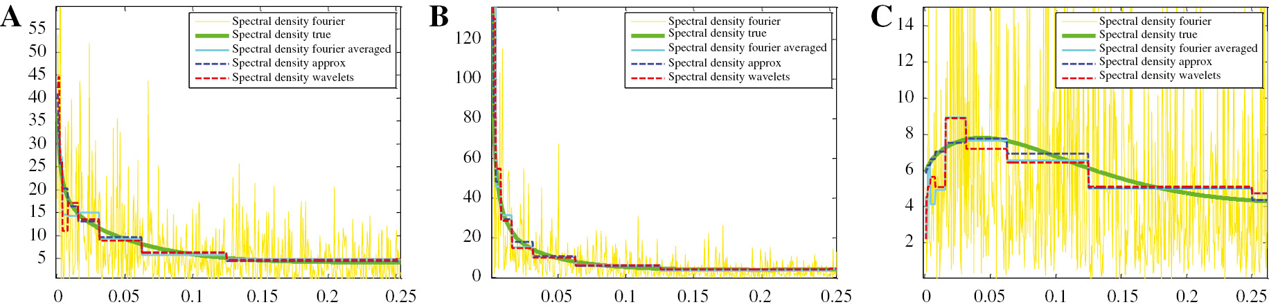
Spectral density estimation (d=0.25/0.45/−0.25), T=2048 (211), level=10, zoom. (A) d=0.25. (B) d=0.45. (C) d=−0.25.

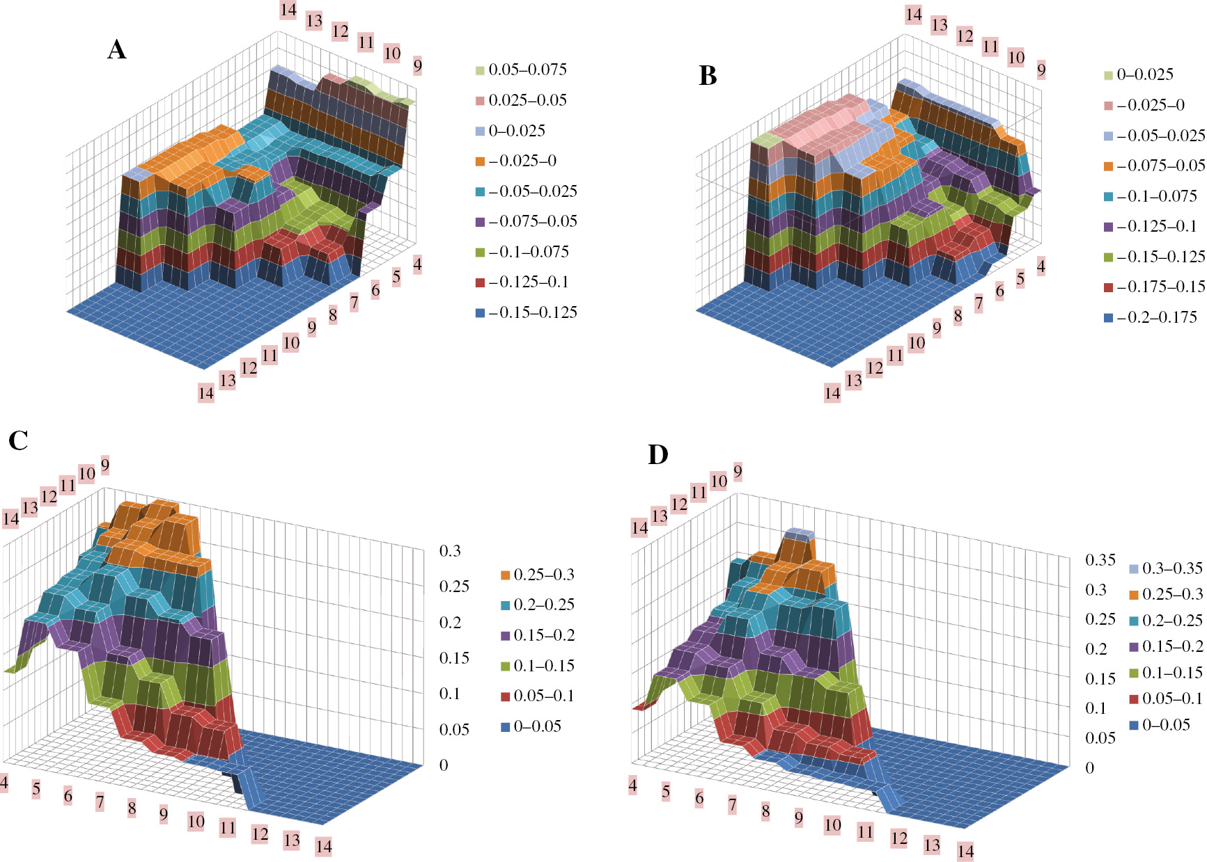
Energy decomposition: (A) Integrals of FIEGARCH spectral density over frequency intervals, and (B) true variances of wavelet coefficients respective to individual levels of decomposition, assuming various levels of long memory (d=0.25, d=0.45, d=−0.25) and the coefficient sets from Table 1.
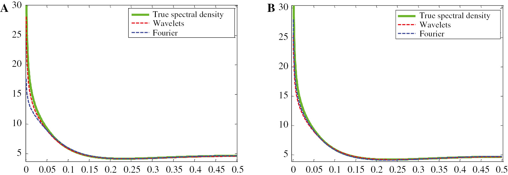
Spectral density estimation in small samples: Wavelets (Level 5) vs. Fourier. (A) T=512 (29), level=5(D4). (B) T=2048 (211), level=5(D4).
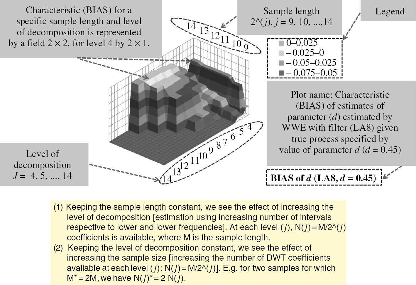
3D plots guide.
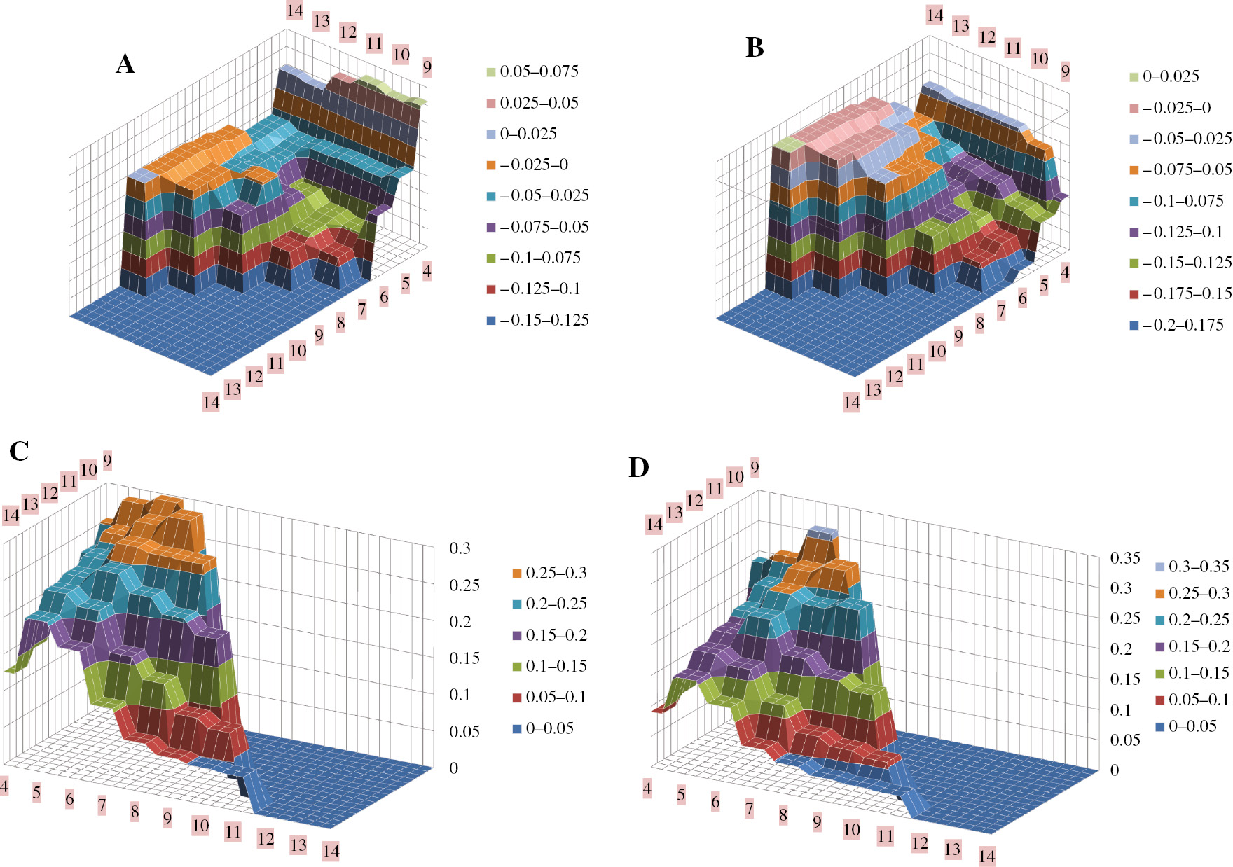
3D plots: Partial decomposition:
3D plots: Partial decomposition:
References
Barunik, J., and L. Vacha. 2015. “Realized Wavelet-Based Estimation of Integrated Variance and Jumps in the Presence of Noise.” Quantitative Finance 15: 1347–1364.10.1080/14697688.2015.1032550Search in Google Scholar
Barunik, J., and L. Vacha. 2016. “Do Co-Jumps Impact Correlations in Currency Markets?” Papers 1602.05489, arXiv.org.10.2139/ssrn.2733736Search in Google Scholar
Barunik, J., T. Krehlik, and L. Vacha. 2016. “Modeling and Forecasting Exchange Rate Volatility in Time-Frequency Domain.” European Journal of Operational Reseach 251: 329–340.10.1016/j.ejor.2015.12.010Search in Google Scholar
Beran, J. 1994. Statistics for Long-Memory Processes. Monographs on statistics and applied probability, 61, Chapman & Hall.Search in Google Scholar
Bollerslev, T. 1986. “Generalized Autoregressive Conditional Heteroskedasticity.” Journal of Econometrics 31: 307–327.10.1016/0304-4076(86)90063-1Search in Google Scholar
Bollerslev, T. 2008. “Glossary to Arch (garch).” CREATES Research Papers 2008-49, School of Economics and Management, University of Aarhus, URL http://ideas.repec.org/p/aah/create/2008-49.html.10.2139/ssrn.1263250Search in Google Scholar
Bollerslev, T., and J. M. Wooldridge. 1992. “Quasi-Maximum Likelihood Estimation and Inference in Dynamic Models with Time-Varying Covariances.” Econometric Reviews 11: 143–172.10.1080/07474939208800229Search in Google Scholar
Bollerslev, T., and H. O. Mikkelsen. 1996. “Modeling and Pricing Long Memory in Stock Market Volatility.” Journal of Econometrics 73: 151–184.10.1016/0304-4076(95)01736-4Search in Google Scholar
Cheung, Y.-W., and F. X. Diebold. 1994. “On Maximum Likelihood Estimation of the Differencing Parameter of Fractionally-Integrated Noise with Unknown Mean.” Journal of Econometrics 62: 301–316.10.1016/0304-4076(94)90026-4Search in Google Scholar
Dahlhaus, R. 1989. “Efficient Parameter Estimation for Self-Similar Processes.” The Annals of Statistics 17: 1749–1766.10.1214/aos/1176347393Search in Google Scholar
Dahlhaus, R. 2006. “Correction: Efficient Parameter Estimation for Self-Similar Processes.” The Annals of Statistics 34: 1045–1047.10.1214/009053606000000182Search in Google Scholar
Donoho, D. L., and I. M. Johnstone. 1994. “Ideal Spatial Adaptation by Wavelet Shrinkage.” Biometrika 81: 425–455.10.1093/biomet/81.3.425Search in Google Scholar
Engle, R. F. 1982. “Autoregressive Conditional Heteroscedasticity with Estimates of the Variance of United Kingdom Inflation.” Econometrica 50: 987–1007.10.2307/1912773Search in Google Scholar
Fan, J., and Y. Wang. 2007. “Multi-Scale Jump and Volatility Analysis for High-Frequency Financial Data.” Journal of the American Statistical Association 102: 1349–1362.10.1198/016214507000001067Search in Google Scholar
Fan, Y., and R. Gençay. 2010. “Unit Root Tests with Wavelets.” Econometric Theory 26: 1305–1331.10.1017/S0266466609990594Search in Google Scholar
Faÿ, G., E. Moulines, F. Roueff, and M. S. Taqqu. 2009. “Estimators of Long-Memory: Fourier versus Wavelets.” Journal of Econometrics 151: 159–177.10.1016/j.jeconom.2009.03.005Search in Google Scholar
Fox, R., and M. S. Taqqu. 1986. “Large-Sample Properties of Parameter Estimates for Strongly Dependent Stationary Gaussian Time Series.” The Annals of Statistics 14: 517–532.10.1214/aos/1176349936Search in Google Scholar
Frederiksen, P. H., and M. O. Nielsen. 2005. “Finite Sample Comparison of Parametric, Semiparametric, and Wavelet Estimators of Fractional Integration.” Econometric Reviews 24: 405–443.10.1080/07474930500405790Search in Google Scholar
Gençay, R., and N. Gradojevic. 2011. “Errors-in-Variables Estimation with Wavelets.” Journal of Statistical Computation and Simulation 81: 1545–1564.10.1080/00949655.2010.495073Search in Google Scholar
Gencay, R., and D. Signori. 2015. “Multi-Scale Tests for Serial Correlation.” Journal of Econometrics 184: 62–80.10.1016/j.jeconom.2014.08.002Search in Google Scholar
Gonzaga, A., and M. Hauser. 2011. “A Wavelet Whittle Estimator of Generalized Long-Memory Stochastic Volatility.” Statistical Methods & Applications 20: 23–48.10.1007/s10260-010-0153-9Search in Google Scholar
Heni, B., and B. Mohamed. 2011. “A Wavelet-Based Approach for Modelling Exchange Rates.” Statistical Methods & Applications 20: 201–220.10.1007/s10260-010-0152-xSearch in Google Scholar
Jensen, M. J. 1999. “An Approximate Wavelet Mle of Short- and Long-Memory Parameters.” Studies in Nonlinear Dynamics Econometrics 3: 5.10.2202/1558-3708.1051Search in Google Scholar
Jensen, M. J. 2000. “An Alternative Maximum Likelihood Estimator of Long-Memory Processes using Compactly Supported Wavelets.” Journal of Economic Dynamics and Control 24: 361–387.10.1016/S0165-1889(99)00010-XSearch in Google Scholar
Johnstone, I. M., and B. W. Silverman. 1997. “Wavelet Threshold Estimators for Data with Correlated Noise.” Journal of the Royal Statistical Society: Series B (Statistical Methodology) 59: 319–351.10.1111/1467-9868.00071Search in Google Scholar
Mancini, C., and F. Calvori. 2012. “Jumps”, in Handbook of Volatility Models and Their Applications, edited by L. Bauwens, C. Hafner and S. Laurent, John Wiley & Sons, Inc., Hoboken, NJ, USA. doi: 10.1002/9781118272039.ch17.10.1002/9781118272039.ch17Search in Google Scholar
Moulines, E., F. Roueff, and M. S. Taqqu. 2008. “A Wavelet Whittle Estimator of the Memory Parameter of a Nonstationary Gaussian Time Series.” The Annals of Statistics 36: 1925–1956.10.1214/07-AOS527Search in Google Scholar
Nielsen, M. O., and P. H. Frederiksen. 2005. “Finite Sample Comparison of Parametric, Semiparametric, and Wavelet Estimators of Fractional Integration.” Econometric Reviews 24: 405–443.10.1080/07474930500405790Search in Google Scholar
Percival, D. P. 1995. “On Estimation of the Wavelet Variance.” Biometrika 82: 619–631.10.1093/biomet/82.3.619Search in Google Scholar
Percival, D. B., and A. T. Walden. 2000. Wavelet Methods for Time Series Analysis (Cambridge Series in Statistical and Probabilistic Mathematics). Cambridge University Press, URL http://www.worldcat.org/isbn/0521685087.Search in Google Scholar
Perez, A., and P. Zaffaroni. 2008. “Finite-Sample Properties of Maximum Likelihood and Whittle Estimators in Egarch and Fiegarch Models.” Quantitative and Qualitative Analysis in Social Sciences 2: 78–97.Search in Google Scholar
Tseng, M. C., and R. Gençay. 2014. “Estimation of Linear Model with One Time-Varying Parameter via Wavelets.”Search in Google Scholar
Whitcher, B. 2004. “Wavelet-Based Estimation for Seasonal Long-Memory Processes.” Technometrics 46: 225–238.10.1198/004017004000000275Search in Google Scholar
Whittle, P. 1962. “Gaussian Estimation in Stationary Time Series.” Bulletin of the International Statistical Institute 39: 105–129.Search in Google Scholar
Wornell, G. W., and A. Oppenheim. 1992. “Estimation of Fractal Signals from Noisy Measurements using Wavelets.” Signal Processing, IEEE Transactions on 40: 611–623.10.1109/78.120804Search in Google Scholar
Xue, Y., R. Gençay, and S. Fagan. 2014. “Jump Detection with Wavelets for High-Frequency Financial Time Series.” Quantitative Finance 14: 1427–1444.10.1080/14697688.2013.830320Search in Google Scholar
Zaffaroni, P. 2009. “Whittle Estimation of Egarch and Other Exponential Volatility Models.” Journal of Econometrics 151: 190–200.10.1016/j.jeconom.2009.03.008Search in Google Scholar
Supplemental Material:
The online version of this article (DOI: https://doi.org/10.1515/snde-2016-0101) offers supplementary material, available to authorized users.
©2017 Walter de Gruyter GmbH, Berlin/Boston
Articles in the same Issue
- VEC-MSF models in Bayesian analysis of short- and long-run relationships
- Detecting capital market convergence clubs
- Changes in persistence, spurious regressions and the Fisher hypothesis
- Money supply and inflation dynamics in the Asia-Pacific economies: a time-frequency approach
- Estimation of long memory in volatility using wavelets