Markov-switching quantile autoregression: a Gibbs sampling approach
-
Xiaochun Liu


Abstract
We extend the class of linear quantile autoregression models by allowing for the possibility of Markov-switching regimes in the conditional distribution of the response variable. We also develop a Gibbs sampling approach for posterior inference by using data augmentation and a location-scale mixture representation of the asymmetric Laplace distribution. Bayesian calculations are easily implemented, because all complete conditional densities used in the Gibbs sampler have closed-form expressions. The proposed Gibbs sampler provides the basis for a stepwise re-estimation procedure that ensures non-crossing quantiles. Monte Carlo experiments and an empirical application to the U.S. real interest rate show that both inference and forecasting are improved when the quantile monotonicity restriction is taken into account.
1 Introduction
The class of linear quantile autoregression (QAR) models of Koenker and Xiao (2006) has proven to be particularly useful for studying asymmetric dynamics and local persistence in many economic and financial time series. Examples include real estate prices (Galvao, Montes-Rojas & Park, 2013; Lee, Lee & Lee, 2014), stock prices and exchange rates (Ferreira, 2011; Baur, Dimpfl & Jung, 2012; Yang, Tu & Zeng, 2014), and more general business cycle and inflation indicators (Manzan, 2015). Our objective in this paper is to extend the class of QAR models by allowing for the possibility of Markov-switching regimes that would influence the conditional quantiles. Indeed, the presence of regime changes in the conditional distribution of the response variable would obviously affect its quantiles. The importance of allowing for such effects can also be recognized from the work of Qu (2008) who proposes testing procedures for structural change in conditional quantiles.
Since the seminal contribution of Hamilton (1989), Markov-switching specifications have become an immensely popular approach to model structural changes in the behaviour of economic and financial time series; see Piger (2009) for an overview. A distinctive feature of the Markov-switching approach is that the regime changes are endogenous to the model, as opposed to being treated exogenously like in the classic approach to structural changes by Chow (1960) which assumes a priori knowledge about how to classify the data between regimes. Building on the earlier work of Goldfeld and Quandt (1973), the Hamilton (1989) approach specifies the regimes as being determined by a discrete-time, discrete-state Markov chain with unknown transition probabilities. This process is assumed to be recurrent, meaning that it can move from one state to any other state at any time. As in the well-known Kalman filter, the unobserved state can be inferred from the observable time series and the sample likelihood function can then be recursively computed. Our specification also complements the related extension of the QAR model proposed by Galvao, Montes-Rojas, and Olmo (2011) in which regime changes are triggered when the time series passes (quantile-specific) threshold values, like in the self-exciting threshold autoregression models of Tong (1983).
Following Albert and Chib (1993), McCulloch and Tsay (1994), Chib (1996), and Frühwirth-Schnatter (2001), we adopt a Bayesian approach to inference based on data augmentation such that the latent states can be analyzed along with the other unknown model parameters through Gibbs sampling. The advantage of the Gibbs sampling approach to the analysis of Markov-switching models has long been recognized. For example, Albert and Chib (1993) remark that such an approach avoids the direct calculation of the likelihood function needed for maximum likelihood estimation. Moreover, the posterior distributions of all unknown parameters (and functions thereof) are fully tractable and easy to simulate from. By treating the unobserved states as missing data, this approach also provides posterior distributions of the states, integrated (by marginalization) over all the other model parameters.
The Bayesian analysis of quantile regression models rests on the connection between the quantile estimation problem and the likelihood function under an asymmetric Laplace distribution, established by Yu and Moyeed (2001) and Tsionas (2003). It is important to note, however, that as in Koenker and Machado (1999) the asymmetric Laplace distribution is not assumed for the data generating process, but is merely used to obtain a quasi-likelihood function. Other examples of such a parametrization for the purpose Bayesian inference include Geraci and Bottai (2007), Kottas and Krnjajić (2009), Yue and Rue (2011), Gerlach, Chen, and Chan (2011), and Chen et al. (2012).
The asymmetric Laplace distribution can be expressed as a location-scale mixture of exponential and normal distributions (Kotz, Kozubowski & Podgórski, 2001). Following Kozumi and Kobayashi (2011), we exploit this representation to develop a Gibbs sampling approach wherein all complete conditional densities have closed-form expressions. An estimate of the marginal likelihood can then be calculated from the Gibbs output using the method of Chib (1995). The marginal likelihood is the key ingredient for model selection and discrimination in Bayesian statistics; see the discussion in Kass and Raftery (1995).
We use the Gibbs sampler to solve the well-known quantile crossing problem that may arise when quantile models are fitted separately for each considered quantile probability level, τ. This common practice of treating the quantile levels independently of one another can yield fitted quantile curves that cross one another, thereby leading to a nonsensical response distribution. Indeed, quantile monotonicity requires the quantiles to be increasing as a function of τ, meaning that any well-defined distribution must necessarily have non-crossing quantiles. Koenker and Xiao (2006), §4 remark that the crossing problem appears more acute in QAR models than in ordinary quantile regressions with exogenous covariates, since the support of the regressors is determined within the autoregressive model.
This quantile crossing problem is potentially worse for non-linear quantile autoregression models, like the threshold specification of Galvao, Montes-Rojas, and Olmo (2011) and the Markov-switching specification developed here. Fortunately, the Gibbs sampler provides the basis for a stepwise re-estimation procedure that ensures non-crossing quantiles. As in Gelfand, Smith, and Lee (1992), draws from the constrained posterior distribution are obtained straightforwardly by retaining the Gibbs draws that satisfy the non-crossing condition when sampling the unconstrained posterior distribution. As far as we know, this is the only way to carry out full Bayesian calculations while avoiding well-nigh impossible numerical integrations over high-dimensional sets defined by complex restrictions involving the model parameters and the data.
It is important to note that the proposal in a related paper by Ye et al. (2016) is to allow for Markov-switching parameters in an ordinary quantile regression with exogenous (independent) regressors, not a quantile autoregression. This is a fundamental difference with what we propose here. Indeed, as we already mentioned, QAR models are more likely to suffer from the quantile crossing problem than ordinary quantile regressions since the regressors are endogenous to the model. Ye et al. (2016) also exploit the asymmetric Laplace connection to devise a (quasi) maximum likelihood estimation (MLE) approach for point estimation, but they do not establish any distributional theory to guide inference. Moreover, their MLE-based approach treats each quantile level separately, which means that it may yield crossing quantiles even though their model is less prone to this problem. In sharp contrast to Ye et al. (2016), our Gibbs sampling approach offers a complete Bayesian methodology not only for estimation, but also inference, model selection, and ensuring non-crossing quantiles in quantile regresison models. It is also important to note that our complete closed-form Gibbs sampling approach can be applied in any quantile regression model with endogenous or exogenous covariates, and whether Markov-switching effects are allowed for or not. In our empirical application, for instance, we estimate non-crossing quantiles with the linear QAR model as well as the Markov-switching QAR model.
The current paper is organized as follows. Section 2 begins by introducing the QAR models of Koenker and Xiao (2006), then shows the asymmetric Laplace connection, and describes the proposed Markov-switching quantile autoregression models. Section 3 develops the Gibbs sampling algorithm based on a location-scale mixture representation of the asymmetric Laplace distribution. There are two variants of the approach, depending on how the state variables are sampled (single- or multi-move Gibbs sampling). Section 4 explains the computation of the marginal likelihood used for model comparisons and the stepwise re-estimation procedure to ensure non-crossing quantiles. Section 5 presents some simulation evidence about the relative performance of the Gibbs samplers in the quantile regression context. Section 6 presents the empirical application to the U.S. real interest rate, which illustrates the gains obtained by enforcing the quantile monotonicity restriction. Section 7 concludes and the computational details are given in the appendices.
2 Markov-switching quantile autoregression
Suppose we have a response variable of interest yt whose time-t conditional quantiles we wish to model as a function of past information. The linear quantile autoregression (QAR) model of Koenker and Xiao (2006) specifies the τth conditional quantile of yt as
where
by choice of c(τ), ϕ1(τ), …, ϕp(τ), and where ρτ(⋅) is the asymmetric absolute deviation loss function defined as
Koenker and Machado (1999) explain that the parameters of linear quantile models can also be estimated by (quasi) maximum likelihood. To see how, consider the QAR(p) model specified in parametric distributional form as
where δ > 0 is a scale parameter and {εt} are i.i.d. according to the asymmetric Laplace distribution with probability density function
The conditional density function of yt for a given τ then becomes
and, conditional on
Since the negative of the loss function appears in the exponent of this expression, maximization of (5) is equivalent to solving the minimization problem in (2). As Yu and Moyeed (2001) and Tsionas (2003) explain, the asymmetric Laplace distribution provides a natural pathway for the Bayesian analysis of quantile regression models. Note also that the value of δ does not matter for the estimation of the correct quantiles by maximizing (5). But rather than fixing it to a constant value, using δ as a free scale parameter clearly makes the assumed asymmetric Laplace distribution more flexible to capture the true (unknown) error distribution. Other examples of such a parametrization for Bayesian inference include Geraci and Bottai (2007), Kottas and Krnjajić (2009), Yue and Rue (2011), Gerlach, Chen, and Chan (2011), and Chen et al. (2012).
The starting point for the developed model is the observation that the QAR(p) model in form (3) is equivalent to
where {εt} are i.i.d. according to the asymmetric Laplace distribution with density (4) so that μ(τ) is the location of the τth conditional quantile in this model with autocorrelated errors. Indeed, since ηt = yt − μ(τ), for all t, (6) can be rewritten as (3) with
where st is a latent variable taking values in the set {1, …, K} according to a Markov chain with one-step transition probability matrix P whose elements are defined as
The term μ(τ, st) in (7) is thus the location of the τth conditional quantile of yt given the past of yt itself and the current regime st. The proposed Markov-switching quantile autoregression (MSQAR) model can then be rewritten as
since ηt = yt − μ(τ, st), for all t, in (7). For a specified τ, the conditional density function of yt given yt−1, …, yt−p and st, …, st−p becomes
where the τth conditional quantile function is given by
Here
The MSQAR model in form (9) can be expressed more compactly as
where
μ1(τ) < μ2(τ) < ⋯ < μK(τ).
All the roots of ϕ(τ, L) = 0 lie outside the unit circle.
pij > 0 for all i, j ∈ {1, …, K}.
Pr(s1 = i) = 1/K for all i ∈ {1, …, K}.
The first three assumptions are standard for Markov-switching time-series models. Assumption 1 ensures the identification of the regimes, while Assumption 2 imposes stationarity given the sequence of state variables. Assumption 3 guarantees that the Markov chain is irreducible, i.e. starting st from an arbitrary state i ∈ {1, …, K}, any state j ∈ {1, …, K} is reachable in finite time. This assumption is also needed for identification purposes because if a state is never visited then the associated parameters cannot be identified. Assumption 4 treats the initial state as a random draw from a uniform distribution, independently of the transition probabilities; see Frühwirth-Schnatter (2006), Ch. 10 for a discussion of the computational advantages of this assumption.
Under these assumptions, the joint density of
which does not constitute the likelihood function. Indeed, the likelihood function for
3 Gibbs sampling
The asymmetric Laplace distribution admits various mixture representations (Kotz, Kozubowski & Podgórski, 2001). Following Kozumi and Kobayashi (2011), the Gibbs sampling algorithm developed here uses a representation based on a mixture of exponential and normal distributions. Specifically, if εt follows the asymmetric Laplace distribution with density (4), then εt can be represented as
with
where
However, as Kozumi and Kobayashi (2011) explain, such an expression is not convenient for Gibbs sampling because the scale parameter δ appears in the conditional location of yt. This issue is resolved by working instead with the reparameterization:
where vt = δet and we let
The model parameters are collected in
where
4 Specification issues
The proposed MSQAR model applies to a specified quantile probability level τ. A typical quantile regression analysis, however, might involve several probability levels τ1 < ⋯ < τq. Two issues arise when several quantile probability levels τ are considered. The first is that the models at the considered quantile levels each yield an inference about the latent Markov chain. This begs the question: which one should be retained?
The second issue is that the fitted quantiles can cross one another, since the models (defined for each τ) are fitted separately. In other words, if the models are estimated separately for each of the q desired probability levels, then the resulting conditional quantile functions may not be monotonically increasing in τ. This is the well-known quantile crossing problem, which obviously leads to a nonsensical response distribution since any distribution must necessarily have non-crossing quantiles in order to be well defined. We solve this problem by proposing a stepwise procedure similar to Wu and Liu (2009), whereby the quantiles are refitted sequentially while constraining the current curve not to cross the previous one.
4.1 Posterior state classification
Our proposal is to first estimate an MSQAR for each quantile level τ1, …, τq separately and to compute the log marginal likelihood estimates
which holds at all admissible points of the parameter space. So for given values
where
Let τi* refer to the model achieving the highest marginal likelihood among the quantile levels
for t = 1, …, T and i = 1, …, K. Note that these posterior state probabilities may be considered as “smoothed” probabilities, since they are based on the full sample, y (Kim & Nelson, 1999, p. 233). The associated sequence of fitted states is denoted
In many practical applications, it may be convenient to simply set
4.2 Non-crossing quantiles
The next step consists of sequentially re-estimating the conditional quantile functions subject to the non-crossing restrictions. Under these constraints the parameter vector
where
and
where
where
It is important to realize that a direct evaluation of this expression is infeasible as it involves numerical integrations over
Fortunately, it is straightforward to obtain a constrained posterior distribution with the Gibbs sampler. Regardless of how complicated a constraint set is, Gelfand, Smith, and Lee (1992) show that the Gibbs sampler can be implemented by identifying the full conditionals under the unconstrained model and then restricting the cross-section. This can be done simply by generating from the unconstrained full conditional and retaining the variate value only if it falls in the cross-section constraint region; see Gelfand, Smith, and Lee (1992) for more details and other examples. In our context, this approach consists of sampling iteratively from
for
for
As far as we know, this is the only way to carry out full Bayesian calculations while avoiding well-nigh impossible numerical integrations over high-dimensional sets defined by complex restrictions. Note also that our method to enforce non-crossing quantiles can be applied in any quantile regression model with endogenous or exogenous covariates, and whether Markov-switching effects are allowed for or not. In our empirical application, for instance, we estimate non-crossing quantiles with the linear QAR model as well as the MSQAR model.
5 Monte Carlo experiments
In this section, we examine the performance of the Gibbs sampler by means of Monte Carlo experiments. We use as data-generating process (DGP) the Garcia and Perron (1996) Markov-switching AR(2) model, given as
where
We set the true values of the parameters appearing in (14) as
We consider the MSQAR(K, p) model in (9), correctly specified with K = 3, p = 2, and nine different quantile levels τ = 0.1, …, 0.9. We also include a misspecified QAR(2) to assess the effect of ignoring the Markov-switching structure. The prior for
From the Gibbs output we obtain
where st is the true state at time t.
Table 1 reports the median along with the corresponding lower 5% and upper 95% quantiles of the PCC statistics across the 400 replications of each DGP configuration. We see that 84 to 94% of states are correctly identified when the quantile level τ is between 0.4 and 0.6, and the PCCs deteriorate as the quantile level becomes more extreme towards either tail. Comparing the distributions, we observe that the best performance is achieved under Student-t errors. For instance, when T = 120 and τ is in the 0.4–0.6 range, the median PCCs under normal and gamma errors are around 80%, while those under the heavier-tailed Student-t errors exceed 90%. It is also interesting to note that increasing the sample size does not affect much the median PCC, but rather has a greater effect of the range of the estimated PCCs. As T doubles from 120 to 240 under each distribution, we can see in general a narrowing of the range between the lower and upper PCC quantiles, while the median remains almost unchanged. This is the same effect also seen when comparing the single- and multi-move samplers. Indeed, the relative computational efficiency of the multi-move relative to the single-move samplers appears most importantly as a reduction in the variance of correctly identified states.
In-sample proportion of correctly identified states under various sample sizes and error distributions: correctly specified MSQAR(3, 2) model.
| Bayesian inference | MLE inference | |||||
|---|---|---|---|---|---|---|
| Single-move sampler | Multi-move sampler | |||||
| τ | T = 120 | T = 240 | T = 120 | T = 240 | T = 120 | T = 240 |
| Panel A: Normal errors | ||||||
| 0.1 | 0.754 (0.296, 0.949) | 0.777 (0.387, 0.924) | 0.788 (0.534, 0.941) | 0.798 (0.592, 0.903) | 0.449 (0.190, 0.720) | 0.473 (0.196, 0.716) |
| 0.2 | 0.771 (0.322, 0.966) | 0.786 (0.327, 0.941) | 0.797 (0.491, 0.949) | 0.790 (0.587, 0.920) | 0.475 (0.177 ,0.791) | 0.511 (0.197, 0.722) |
| 0.3 | 0.780 (0.314, 0.941) | 0.790 (0.454, 0.916) | 0.805 (0.491, 0.966) | 0.811 (0.580, 0.937) | 0.572 (0.267, 0.845) | 0.598 (0.284, 0.773) |
| 0.4 | 0.805 (0.500, 0.932) | 0.798 (0.584, 0.908) | 0.839 (0.550, 0.975) | 0.853 (0.654, 0.945) | 0.555 (0.261, 0.854) | 0.627 (0.249, 0.810) |
| 0.5 | 0.812 (0.559, 0.941) | 0.819 (0.630, 0.916) | 0.873 (0.635, 0.975) | 0.875 (0.726, 0.958) | 0.579 (0.269, 0.886) | 0.645 (0.251, 0.835) |
| 0.6 | 0.805 (0.406, 0.949) | 0.811 (0.504, 0.924) | 0.856 (0.609, 0.975) | 0.861 (0.680, 0.958) | 0.552 (0.267, 0.880) | 0.641 (0.242, 0.844) |
| 0.7 | 0.788 (0.364, 0.958) | 0.811 (0.353, 0.933) | 0.831 (0.559, 0.966) | 0.840 (0.638, 0.941) | 0.564 (0.269, 0.836) | 0.626 (0.251, 0.787) |
| 0.8 | 0.767 (0.336, 0.966) | 0.803 (0.356, 0.950) | 0.822 (0.525, 0.958) | 0.819 (0.618, 0.929) | 0.462 (0.174, 0.782) | 0.529 (0.279, 0.772) |
| 0.9 | 0.763 (0.303, 0.966) | 0.773 (0.339, 0.937) | 0.822 (0.584, 0.958) | 0.817 (0.639, 0.920) | 0.455 (0.207, 0.740) | 0.545 (0.191, 0.730) |
| Average | 0.782 (0.377, 0.946) | 0.796 (0.437, 0.923) | 0.825 (0.553, 0.956) | 0.829 (0.634, 0.930) | 0.518 (0.230, 0.817) | 0.577 (0.242, 0.779) |
| Panel B: Student-t errors | ||||||
| 0.1 | 0.856 (0.610, 0.958) | 0.845 (0.680, 0.945) | 0.864 (0.635, 0.966) | 0.869 (0.706, 0.941) | 0.503 (0.179, 0.783) | 0.493 (0.221, 0.775) |
| 0.2 | 0.881 (0.635, 0.966) | 0.874 (0.718, 0.958) | 0.886 (0.695, 0.975) | 0.888 (0.744, 0.958) | 0.552 (0.228, 0.884) | 0.601 (0.235, 0.885) |
| 0.3 | 0.907 (0.669, 0.983) | 0.908 (0.777, 0.975) | 0.915 (0.737, 0.983) | 0.917 (0.811, 0.975) | 0.667 (0.402, 0.936) | 0.675 (0.408, 0.919) |
| 0.4 | 0.924 (0.576, 0.992) | 0.929 (0.651, 0.979) | 0.932 (0.805, 0.992) | 0.935 (0.861, 0.979) | 0.689 (0.386, 0.937) | 0.743 (0.483, 0.935) |
| 0.5 | 0.932 (0.613, 0.992) | 0.941 (0.720, 0.983) | 0.941 (0.839, 0.992) | 0.945 (0.874, 0.987) | 0.668 (0.378, 0.954) | 0.765 (0.476, 0.947) |
| 0.6 | 0.941 (0.600, 0.992) | 0.941 (0.702, 0.987) | 0.941 (0.831, 0.992) | 0.941 (0.865, 0.987) | 0.676 (0.375, 0.948) | 0.719 (0.501, 0.949) |
| 0.7 | 0.924 (0.686, 0.992) | 0.920 (0.765, 0.979) | 0.924 (0.780, 0.992) | 0.924 (0.819, 0.983) | 0.666 (0.380, 0.932) | 0.707 (0.403, 0.942) |
| 0.8 | 0.898 (0.703, 0.975) | 0.891 (0.760, 0.971) | 0.898 (0.746, 0.983) | 0.895 (0.773, 0.971) | 0.567 (0.287, 0.908) | 0.576 (0.314, 0.915) |
| 0.9 | 0.873 (0.694, 0.966) | 0.866 (0.706, 0.954) | 0.881 (0.712, 0.967) | 0.886 (0.718, 0.962) | 0.499 (0.192, 0.819) | 0.534 (0.244, 0.870) |
| Average | 0.904 (0.642, 0.975) | 0.901 (0.719, 0.964) | 0.909 (0.753, 0.978) | 0.911 (0.796, 0.966) | 0.609 (0.314, 0.899) | 0.645 (0.366, 0.908) |
| Panel C: Gamma errors | ||||||
| 0.1 | 0.720 (0.332, 0.967) | 0.739 (0.256, 0.945) | 0.814 (0.551, 0.966) | 0.813 (0.563, 0.929) | 0.484 (0.197, 0.769) | 0.535 (0.219, 0.823) |
| 0.2 | 0.742 (0.288, 0.958) | 0.775 (0.298, 0.945) | 0.805 (0.533, 0.967) | 0.811 (0.546, 0.937) | 0.624 (0.295, 0.823) | 0.632 (0.318, 0.832) |
| 0.3 | 0.780 (0.304, 0.958) | 0.794 (0.349, 0.933) | 0.818 (0.500, 0.975) | 0.828 (0.538, 0.950) | 0.626 (0.279, 0.839) | 0.652 (0.310, 0.863) |
| 0.4 | 0.788 (0.414, 0.966) | 0.803 (0.538, 0.929) | 0.839 (0.559, 0.983) | 0.845 (0.613, 0.962) | 0.714 (0.376, 0.879) | 0.723 (0.424, 0.857) |
| 0.5 | 0.807 (0.508, 0.958) | 0.814 (0.592, 0.916) | 0.864 (0.619, 0.983) | 0.876 (0.701, 0.962) | 0.709 (0.393, 0.889) | 0.748 (0.492, 0.855) |
| 0.6 | 0.790 (0.340, 0.941) | 0.805 (0.499, 0.941) | 0.864 (0.635, 0.983) | 0.878 (0.706, 0.962) | 0.712 (0.381, 0.885) | 0.727 (0.490, 0.876) |
| 0.7 | 0.780 (0.381, 0.958) | 0.786 (0.420, 0.929) | 0.839 (0.576, 0.975) | 0.849 (0.660, 0.946) | 0.612 (0.386, 0.877) | 0.710 (0.413, 0.859) |
| 0.8 | 0.758 (0.347, 0.949) | 0.771 (0.398, 0.954) | 0.805 (0.508, 0.958) | 0.815 (0.609, 0.929) | 0.529 (0.317, 0.817) | 0.617 (0.350, 0.822) |
| 0.9 | 0.729 (0.311, 0.975) | 0.754 (0.356, 0.950) | 0.805 (0.550, 0.949) | 0.807 (0.609, 0.916) | 0.486 (0.201, 0.729) | 0.493 (0.268, 0.738) |
| Average | 0.766 (0.358, 0.952) | 0.782 (0.411, 0.933) | 0.828 (0.559, 0.965) | 0.835 (0.616, 0.938) | 0.611 (0.315, 0.832) | 0.641 (0.359, 0.832) |
This table shows the median of the in-sample PCCs, defined in (15), across 400 replications of each DGP, while the numbers in parenthesis are the corresponding 5% and 95% quantiles.
The accuracy of estimation is further assessed by examining the deviations between the true conditional quantile
where
In-sample MADE under various sample sizes and error distributions: correctly specified MSQAR(3, 2) model.
| Bayesian inference | MLE inference | |||||
|---|---|---|---|---|---|---|
| Single-move sampler | Multi-move sampler | |||||
| τ | T = 120 | T = 240 | T = 120 | T = 240 | T = 120 | T = 240 |
| Panel A: Normal errors | ||||||
| 0.1 | 1.045 (0.753, 1.547) | 0.980 (0.702, 1.341) | 1.008 (0.731, 1.530) | 0.945 (0.680, 1.275) | 1.411 (1.048, 1.793) | 1.373 (1.106, 1.661) |
| 0.2 | 0.931 (0.637, 1.524) | 0.859 (0.622, 1.256) | 0.919 (0.632, 1.332) | 0.847 (0.609, 1.193) | 1.227 (0.925, 1.558) | 1.190 (0.949, 1.415) |
| 0.3 | 0.890 (0.516, 1.434) | 0.809 (0.504, 1.313) | 0.829 (0.495, 1.317) | 0.763 (0.494, 1.077) | 1.147 (0.894, 1.451) | 1.116 (0.894, 1.314) |
| 0.4 | 0.828 (0.353, 1.425) | 0.758 (0.418, 1.353) | 0.647 (0.346, 1.162) | 0.622 (0.376, 0.984) | 1.123 (0.877, 1.391) | 1.089 (0.883, 1.287) |
| 0.5 | 0.861 (0.298, 1.473) | 0.774 (0.355, 1.421) | 0.544 (0.235, 1.083) | 0.514 (0.287, 0.856) | 1.127 (0.873, 1.409) | 1.085 (0.882, 1.279) |
| 0.6 | 0.867 (0.385, 1.466) | 0.735 (0.388, 1.374) | 0.650 (0.360, 1.164) | 0.609 (0.352, 0.949) | 1.150 (0.885, 1.431) | 1.103 (0.865, 1.324) |
| 0.7 | 0.910 (0.538, 1.511) | 0.828 (0.546, 1.286) | 0.827 (0.519, 1.280) | 0.769 (0.522, 1.051) | 1.205 (0.909, 1.580) | 1.152 (0.885, 1.409) |
| 0.8 | 0.993 (0.699, 1.557) | 0.915 (0.661, 1.206) | 0.975 (0.668, 1.469) | 0.902 (0.639, 1.137) | 1.306 (0.971, 1.630) | 1.243 (0.945, 1.522) |
| 0.9 | 1.113 (0.829, 1.633) | 1.046 (0.782, 1.306) | 1.092 (0.796, 1.545) | 1.028 (0.775, 1.274) | 1.555 (1.130, 2.040) | 1.470 (1.103, 1.830) |
| Average | 0.937 (0.556, 1.503) | 0.856 (0.553, 1.313) | 0.832 (0.531, 1.316) | 0.777 (0.526, 1.083) | 1.250 (0.975, 1.618) | 1.202 (0.973, 1.475) |
| Panel B: Student-t errors | ||||||
| 0.1 | 0.816 (0.559, 1.289) | 0.777 (0.511, 1.088) | 0.801 (0.533, 1.282) | 0.752 (0.499, 1.040) | 1.255 (0.755, 1.975) | 1.186 (0.708, 1.877) |
| 0.2 | 0.615 (0.372, 1.049) | 0.592 (0.358, 0.849) | 0.604 (0.343, 1.022) | 0.569 (0.349, 0.832) | 1.060 (0.596, 1.836) | 0.987 (0.589, 1.821) |
| 0.3 | 0.470 (0.245, 0.899) | 0.439 (0.237, 0.694) | 0.444 (0.240, 0.795) | 0.427 (0.230, 0.643) | 0.969 (0.504, 1.617) | 0.909 (0.478, 1.523) |
| 0.4 | 0.381 (0.178, 0.901) | 0.336 (0.174, 0.873) | 0.336 (0.173, 0.651) | 0.316 (0.173, 0.519) | 0.949 (0.450, 1.691) | 0.958 (0.430, 1.683) |
| 0.5 | 0.324 (0.143, 0.841) | 0.302 (0.160, 0.923) | 0.290 (0.143, 0.589) | 0.278 (0.146, 0.467) | 1.017 (0.777, 1.292) | 0.990 (0.794, 1.210) |
| 0.6 | 0.359 (0.160, 0.847) | 0.322 (0.150, 0.861) | 0.340 (0.154, 0.627) | 0.298 (0.146, 0.525) | 1.036 (0.773, 1.307) | 1.011 (0.794, 1.246) |
| 0.7 | 0.457(0.288, 0.900) | 0.420 (0.219, 0.746) | 0.430 (0.214, 0.754) | 0.397 (0.210, 0.671) | 1.089 (0.795, 1.379) | 1.063 (0.815, 1.307) |
| 0.8 | 0.609 (0.372, 0.988) | 0.569 (0.333, 0.875) | 0.594 (0.356, 0.940) | 0.549 (0.331, 0.838) | 1.200 (0.853, 1.592) | 1.170 (0.534, 2.427) |
| 0.9 | 0.853 (0.570, 1.388) | 0.801 (0.540, 1.104) | 0.824 (0.531, 1.275) | 0.773 (0.526, 1.061) | 1.288 (0.732, 2.452) | 1.090 (0.695, 1.872) |
| Average | 0.542 (0.320, 1.005) | 0.506 (0.298, 0.885) | 0.518 (0.298, 0.877) | 0.484 (0.29, 0.728) | 1.096 (0.726, 1.716) | 1.041 (0.679, 1.698) |
| Panel C: Gamma errors | ||||||
| 0.1 | 0.769 (0.542, 1.075) | 0.682 (0.467, 0.931) | 0.769 (0.527, 1.048) | 0.670 (0.466, 0.917) | 1.247 (0.574, 2.168) | 1.152 (0.493, 2.110) |
| 0.2 | 0.802 (0.572, 1.144) | 0.721 (0.507, 1.037) | 0.797 (0.544, 1.076) | 0.711 (0.500, 0.953) | 1.101 (0.577, 1.951) | 1.039 (0.512, 1.791) |
| 0.3 | 0.824 (0.560, 1.396) | 0.754 (0.493, 1.153) | 0.785 (0.512, 1.124) | 0.714 (0.475, 0.958) | 1.080 (0.630, 1.737) | 1.059 (0.804, 1.273) |
| 0.4 | 0.853 (0.512, 1.437) | 0.799 (0.475, 1.353) | 0.745 (0.449, 1.082) | 0.666 (0.413, 0.960) | 1.080 (0.822, 1.350) | 1.039 (0.810, 1.252) |
| 0.5 | 0.888 (0.381, 1.467) | 0.840 (0.364, 1.481) | 0.632 (0.347, 1.006) | 0.561 (0.312, 0.879) | 1.087 (0.825, 1.354) | 1.036 (0.804, 1.255) |
| 0.6 | 0.877 (0.322, 1.452) | 0.822 (0.322, 1.377) | 0.575 (0.237, 1.033) | 0.508 (0.266, 0.879) | 1.109 (0.857, 1.394) | 1.057 (0.819, 1.292) |
| 0.7 | 0.889 (0.450, 1.419) | 0.810 (0.429, 1.336) | 0.716 (0.386, 1.237) | 0.677 (0.408, 1.022) | 1.158 (0.871, 1.480) | 1.106 (0.834, 1.363) |
| 0.8 | 1.080 (0.700, 1.603) | 0.976 (0.624, 1.394) | 1.021 (0.628, 1.534) | 0.923 (0.596, 1.272) | 1.281 (0.939, 1.639) | 1.211 (0.888, 1.493) |
| 0.9 | 1.349 (0.937, 1.874) | 1.244 (0.852, 1.687) | 1.304 (0.911, 1.870) | 1.203 (0.823, 1.572) | 1.582 (1.144, 2.119) | 1.464 (1.051, 1.813) |
| Average | 0.925 (0.552, 1.424) | 0.849 (0.503, 1.301) | 0.816 (0.504, 1.218) | 0.737 (0.473, 1.041) | 1.192 (0.840, 1.720) | 1.129 (0.812, 1.551) |
This table reports the median of the in-sample MADEs, defined in (16), across DGP replications. The numbers in parenthesis are the lower 5% and upper 95% quantiles of the 400 corresponding MADEs.
We see that using the asymmetric Laplace distribution as the likelihood achieves the greatest estimation precision as defined by (16) for the central quantiles under Student-t errors. In this case, the MADEs are around 0.30, while they exceed 0.50 under normal and gamma distributed errors, and sometimes by far. As expected, the MADEs appear roughly symmetric under normal and Student-t errors, i.e. the estimated MADEs are about the same whether τ equals 0.1 or 0.9, 0.2 or 0.8, etc. On the contrary, the MADEs for the gamma distribution are consistently higher in the right tail, e.g. when τ = 0.9. This happens because the distribution is skewed to the right, meaning that there are relatively fewer observations in the right tail compared to the left tail.
Of course, increasing the sample size improves the estimation precision at all quantile levels τ. This is readily seen from the upper 95% MADE quantiles which tend to decrease as T doubles from 120 to 240. Observe further that the multi-move sampler appears preferable, since these upper 95% limits are systematically lower than with the single-move sampler. We therefore leave aside the single-move sampler and proceed to the empirical application with the computationally more efficient multi-move sampler.
Table 3 provides a comparison of the in-sample MADEs of the misspecified QAR(2) model, obtained by Gibbs sampling and MLE.[5] The pattern is clear: even with the misspecified QAR(2) model, the Bayesian approach yields smaller in-sample median MADEs relative to the MLE approach. Focusing on the averages, we see that the pattern holds for each T and error distribution.
In-sample MADE under various sample sizes and error distributions: misspecified QAR(2) model.
| Bayesian inference | MLE inference | |||
|---|---|---|---|---|
| τ | T = 120 | T = 240 | T = 120 | T = 240 |
| Panel A: Normal errors | ||||
| 0.1 | 1.431 (0.914, 2.227) | 1.359 (0.832, 2.117) | 1.592 (1.167, 2.487) | 1.581 (1.224, 2.371) |
| 0.2 | 1.256 (0.793, 2.017) | 1.269 (0.813, 2.016) | 1.392 (1.060, 2.193) | 1.376 (1.068, 2.097) |
| 0.3 | 1.213 (0.705, 1.973) | 1.218 (0.766, 1.935) | 1.320 (1.055, 2.089) | 1.307 (1.047, 2.025) |
| 0.4 | 1.237 (0.718, 2.001) | 1.235 (0.728, 1.999) | 1.296 (1.036, 2.060) | 1.281 (1.030, 2.002) |
| 0.5 | 1.262 (0.659, 2.184) | 1.259 (0.733, 2.083) | 1.297 (1.020, 2.263) | 1.279 (1.038, 1.990) |
| 0.6 | 1.324 (0.709, 2.308) | 1.340 (0.713, 2.630) | 1.324 (1.020, 2.409) | 1.298 (1.048, 2.445) |
| 0.7 | 1.352 (0.759, 2.551) | 1.384 (0.773, 2.548) | 1.379 (1.049, 2.671) | 1.346 (1.062, 2.410) |
| 0.8 | 1.366 (0.826, 2.540) | 1.360 (0.770, 2.553) | 1.483 (1.110, 2.711) | 1.449 (1.077, 2.646) |
| 0.9 | 1.654 (0.897, 3.270) | 1.521 (0.829, 3.072) | 1.752 (1.286, 3.726) | 1.703 (1.231, 3.574) |
| Average | 1.343 (0.775, 2.341) | 1.327 (0.773, 2.328) | 1.426 (1.089, 2.512) | 1.402 (1.092, 2.395) |
| Panel B: Student-t errors | ||||
| 0.1 | 1.417 (0.979, 1.978) | 1.376 (1.027, 1.856) | 1.607 (1.157, 2.589) | 1.600 (1.215, 2.528) |
| 0.2 | 1.173 (0.856, 1.510) | 1.147 (0.902, 1.457) | 1.348 (0.994, 2.174) | 1.345 (1.068, 2.130) |
| 0.3 | 1.074 (0.807, 1.370) | 1.047 (0.839, 1.275) | 1.241 (0.922, 2.033) | 1.228 (0.992, 1.973) |
| 0.4 | 1.031 (0.780, 1.302) | 1.007 (0.805, 1.227) | 1.193 (0.902, 1.958) | 1.179 (0.957, 1.893) |
| 0.5 | 1.043 (0.419, 2.088) | 1.039 (0.408, 2.131) | 1.184 (0.904, 1.952) | 1.170 (0.949, 1.880) |
| 0.6 | 1.146 (0.413, 2.634) | 1.105 (0.437, 2.393) | 1.204 (0.918, 1.963) | 1.191 (0.972, 1.912) |
| 0.7 | 1.186 (0.479, 2.699) | 1.114 (0.442, 2.602) | 1.259 (0.961, 2.064) | 1.251 (1.009, 2.002) |
| 0.8 | 1.243 (0.567, 2.843) | 1.185 (0.900, 1.504) | 1.398 (1.018, 2.309) | 1.383 (1.053, 2.182) |
| 0.9 | 1.505 (1.024, 2.023) | 1.468 (1.086, 1.880) | 1.717 (1.209, 2.815) | 1.710 (1.280, 2.638) |
| Average | 1.202 (0.702, 2.049) | 1.165 (0.760, 1.813) | 1.350 (0.999, 2.206) | 1.340 (1.055, 2.126) |
| Panel C: Gamma errors | ||||
| 0.1 | 1.366 (0.992, 1.754) | 1.320 (0.978, 1.609) | 1.594 (1.151, 2.542) | 1.560 (1.106, 2.377) |
| 0.2 | 1.162 (0.878, 1.449) | 1.126 (0.833, 1.346) | 1.345 (1.014, 2.138) | 1.317 (0.950, 2.051) |
| 0.3 | 1.106 (0.845, 1.386) | 1.088 (0.573, 1.896) | 1.278 (0.984, 2.055) | 1.248 (0.939, 1.974) |
| 0.4 | 1.128 (0.658, 1.806) | 1.093 (0.602, 1.701) | 1.259 (0.980, 2.023) | 1.227 (0.960, 1.949) |
| 0.5 | 1.185 (0.626, 2.049) | 1.159 (0.634, 1.951) | 1.262 (0.994, 2.034) | 1.227 (0.977, 1.947) |
| 0.6 | 1.310 (0.671, 2.575) | 1.277 (0.653, 2.427) | 1.284 (1.007, 2.102) | 1.247 (0.979, 1.998) |
| 0.7 | 1.362 (0.720, 2.507) | 1.398 (0.720, 2.631) | 1.338 (1.000, 2.172) | 1.294 (0.988, 2.067) |
| 0.8 | 1.449 (0.867, 2.540) | 1.381 (0.785, 2.578) | 1.454 (1.048, 2.364) | 1.407 (1.022, 2.199) |
| 0.9 | 1.694 (1.109, 2.659) | 1.598 (1.011, 2.568) | 1.752 (1.229, 2.844) | 1.649 (1.142, 2.502) |
| Average | 1.306 (0.818, 2.080) | 1.271 (0.754, 2.078) | 1.396 (1.045, 2.253) | 1.353 (1.007, 2.118) |
This table reports the median of the in-sample MADEs, defined in (16), across DGP replications. The numbers in parenthesis are the lower 5% and upper 95% quantiles of the 400 corresponding MADEs.
Table 4–Table 6 provide an assessment of the out-of-sample accuracy of the model forecasts. For this purpose we use the DGP in (14) to simulate trajectories of length T + 1, and then, using only the data up to time T, we forecast the quantiles of yT + 1. Table 4 reports the average of
Out-of-sample proportion of correctly identified states under various sample sizes and error distributions: correctly specified MSQAR(3, 2) model.
| Bayesian inference | MLE inference | |||||
|---|---|---|---|---|---|---|
| Single-move sampler | Multi-move sampler | |||||
| τ | T = 120 | T = 240 | T = 120 | T = 240 | T = 120 | T = 240 |
| Panel A: Normal errors | ||||||
| 0.1 | 0.670 | 0.700 | 0.682 | 0.720 | 0.700 | 0.710 |
| 0.2 | 0.650 | 0.700 | 0.698 | 0.720 | 0.708 | 0.740 |
| 0.3 | 0.628 | 0.680 | 0.708 | 0.738 | 0.693 | 0.705 |
| 0.4 | 0.630 | 0.660 | 0.755 | 0.762 | 0.708 | 0.740 |
| 0.5 | 0.610 | 0.620 | 0.752 | 0.780 | 0.633 | 0.683 |
| 0.6 | 0.622 | 0.675 | 0.742 | 0.782 | 0.668 | 0.683 |
| 0.7 | 0.628 | 0.720 | 0.702 | 0.750 | 0.673 | 0.730 |
| 0.8 | 0.668 | 0.730 | 0.705 | 0.742 | 0.668 | 0.703 |
| 0.9 | 0.712 | 0.760 | 0.712 | 0.748 | 0.655 | 0.723 |
| Average | 0.646 | 0.694 | 0.717 | 0.749 | 0.678 | 0.713 |
| Panel B: Student-t errors | ||||||
| 0.1 | 0.740 | 0.770 | 0.735 | 0.775 | 0.505 | 0.565 |
| 0.2 | 0.745 | 0.792 | 0.770 | 0.795 | 0.563 | 0.548 |
| 0.3 | 0.768 | 0.825 | 0.782 | 0.830 | 0.535 | 0.523 |
| 0.4 | 0.765 | 0.825 | 0.818 | 0.862 | 0.513 | 0.550 |
| 0.5 | 0.790 | 0.830 | 0.832 | 0.862 | 0.530 | 0.580 |
| 0.6 | 0.812 | 0.832 | 0.840 | 0.865 | 0.560 | 0.548 |
| 0.7 | 0.802 | 0.845 | 0.828 | 0.860 | 0.588 | 0.578 |
| 0.8 | 0.805 | 0.825 | 0.805 | 0.828 | 0.638 | 0.585 |
| 0.9 | 0.782 | 0.805 | 0.790 | 0.805 | 0.623 | 0.590 |
| Average | 0.779 | 0.817 | 0.800 | 0.831 | 0.562 | 0.563 |
| Panel C: Gamma errors | ||||||
| 0.1 | 0.740 | 0.740 | 0.740 | 0.770 | 0.623 | 0.625 |
| 0.2 | 0.712 | 0.715 | 0.735 | 0.745 | 0.623 | 0.608 |
| 0.3 | 0.658 | 0.700 | 0.748 | 0.765 | 0.578 | 0.575 |
| 0.4 | 0.590 | 0.655 | 0.760 | 0.778 | 0.595 | 0.595 |
| 0.5 | 0.608 | 0.630 | 0.752 | 0.768 | 0.573 | 0.600 |
| 0.6 | 0.605 | 0.650 | 0.762 | 0.770 | 0.575 | 0.570 |
| 0.7 | 0.622 | 0.692 | 0.728 | 0.762 | 0.585 | 0.635 |
| 0.8 | 0.630 | 0.715 | 0.688 | 0.758 | 0.663 | 0.588 |
| 0.9 | 0.680 | 0.750 | 0.698 | 0.755 | 0.633 | 0.660 |
| Average | 0.649 | 0.694 | 0.735 | 0.763 | 0.605 | 0.606 |
For each T and τ, the unconstrained MSQAR model is used to obtain an out-of-sample forecast
Out-of-sample MADE under various sample sizes and error distributions: correctly specified MSQAR(3, 2) model.
| Unconstrained Bayesian inference | Constrained Bayesian inference | MLE inference | ||||
|---|---|---|---|---|---|---|
| τ | T = 120 | T = 240 | T = 120 | T = 240 | T = 120 | T = 240 |
| Panel A: Normal errors | ||||||
| 0.1 | 1.199 (0.389, 3.422) | 1.195 (0.302, 2.700) | 1.137 (0.306, 2.742) | 1.043 (0.247, 2.282) | 1.442 (0.609, 3.065) | 1.421 (0.590, 2.972) |
| 0.2 | 1.117 (0.421, 3.016) | 1.078 (0.357, 2.505) | 1.036 (0.298, 2.378) | 1.025 (0.242, 2.015) | 1.224 (0.475, 3.021) | 1.223 (0.462, 2.946) |
| 0.3 | 1.066 (0.462, 2.063) | 0.975 (0.401, 2.063) | 0.946 (0.278, 1.902) | 0.932 (0.241, 1.517) | 1.121 (0.403, 3.012) | 1.119 (0.384, 2.781) |
| 0.4 | 0.880 (0.283, 2.186) | 0.853 (0.259, 2.184) | 0.818 (0.162 1.924) | 0.798 (0.122, 1.739) | 1.076 (0.329, 3.093) | 1.084 (0.316, 2.615) |
| 0.5 | 0.794 (0.236, 1.682) | 0.782 (0.209, 1.671) | 0.686 (0.114, 1.917) | 0.640 (0.082, 1.505) | 1.091 (0.296, 3.042) | 1.075 (0.281, 2.627) |
| 0.6 | 0.939 (0.327, 2.142) | 0.774 (0.269, 2.122) | 0.792 (0.151, 2.086) | 0.701 (0.113, 2.062) | 1.141 (0.354, 3.061) | 1.074 (0.335, 2.689) |
| 0.7 | 1.109 (0.555, 2.264) | 0.926 (0.491, 2.174) | 0.955 (0.220, 2.204) | 0.848 (0.193, 2.155) | 1.215 (0.462, 3.071) | 1.118 (0.446, 2.820) |
| 0.8 | 1.233 (0.598, 2.354) | 1.002 (0.539, 2.344) | 1.104 (0.303, 2.277) | 0.992 (0.277, 1.895) | 1.333 (0.499, 3.045) | 1.203 (0.481, 2.909) |
| 0.9 | 1.376 (0.551, 2.909) | 1.154 (0.483, 2.479) | 1.211 (0.252, 2.762) | 1.091 (0.218, 2.387) | 1.635 (0.572, 3.078) | 1.439 (0.560, 2.975) |
| Average | 1.079 (0.424, 2.344) | 0.971 (0.368, 2.129) | 0.965 (0.231, 2.265) | 0.897 (0.193, 1.950) | 1.253 (0.451, 3.047) | 1.195 (0.435, 2.824) |
| Panel B: Student-t errors | ||||||
| 0.1 | 1.134 (0.511, 3.082) | 0.948 (0.423, 2.752) | 0.948 (0.232, 2.395) | 0.838 (0.181, 2.206) | 1.401 (0.514, 2.975) | 1.288 (0.499, 2.902) |
| 0.2 | 0.885 (0.446, 2.359) | 0.761 (0.354, 1.906) | 0.752 (0.279, 1.870) | 0.644 (0.230, 1.223) | 1.207 (0.464, 3.087) | 1.181 (0.446, 3.027) |
| 0.3 | 0.824 (0.424, 1.956) | 0.637 (0.368, 1.926) | 0.631 (0.208, 1.851) | 0.498 (0.167, 1.193) | 1.094 (0.435, 3.018) | 1.096 (0.415, 2.973) |
| 0.4 | 0.718 (0.298, 1.887) | 0.526 (0.230, 1.815) | 0.509 (0.131, 1.825) | 0.384 (0.102, 1.478) | 1.067 (0.300, 2.948) | 1.034 (0.286, 2.833) |
| 0.5 | 0.669 (0.307, 1.796) | 0.528 (0.254, 1.416) | 0.454 (0.130, 1.791) | 0.305 (0.079, 1.419) | 1.093 (0.344, 2.860) | 1.042 (0.327, 2.830) |
| 0.6 | 0.639 (0.222, 1.706) | 0.540 (0.152, 1.606) | 0.461 (0.118, 1.876) | 0.334 (0.070, 1.448) | 1.122 (0.350, 2.978) | 1.071 (0.332, 2.873) |
| 0.7 | 0.721 (0.494, 2.180) | 0.616 (0.459, 1.688) | 0.552 (0.241, 1.839) | 0.408 (0.189, 1.227) | 1.166 (0.424, 3.041) | 1.135 (0.414, 2.988) |
| 0.8 | 0.868 (0.470, 2.623) | 0.760 (0.432, 1.949) | 0.699 (0.260, 1.995) | 0.561 (0.218, 1.175) | 1.289 (0.494, 2.985) | 1.252 (0.479, 2.927) |
| 0.9 | 1.116 (0.506, 3.209) | 0.981 (0.436, 2.753) | 0.991 (0.217, 2.736) | 0.809 (0.183, 2.335) | 1.386 (0.609, 2.968) | 1.266 (0.597, 2.912) |
| Average | 0.842 (0.409, 2.266) | 0.699 (0.345, 1.979) | 0.666 (0.202, 2.019) | 0.531 (0.158, 1.522) | 1.203 (0.453, 2.940) | 1.152 (0.438, 2.877) |
| Panel C: Gamma errors | ||||||
| 0.1 | 0.882 (0.449, 2.542) | 0.802 (0.370, 1.742) | 0.763 (0.211, 0.915) | 0.688 (0.176, 0.466) | 1.248 (0.606, 2.828) | 1.235 (0.590, 2.803) |
| 0.2 | 0.888 (0.627, 2.298) | 0.836 (0.543, 1.531) | 0.794 (0.285, 0.902) | 0.731 (0.231, 0.516) | 1.137 (0.507, 2.671) | 1.069 (0.495, 2.601) |
| 0.3 | 0.906 (0.435, 1.764) | 0.811 (0.366, 1.753) | 0.797 (0.312, 0.945) | 0.738 (0.266, 0.410) | 1.071 (0.351, 2.752) | 1.043 (0.339, 2.712) |
| 0.4 | 0.856 (0.392, 2.063) | 0.795 (0.334, 1.892) | 0.803 (0.161, 1.956) | 0.768 (0.110, 1.779) | 1.072 (0.369, 2.553) | 1.027 (0.356, 2.488) |
| 0.5 | 0.846 (0.305, 2.313) | 0.810 (0.235, 2.113) | 0.727 (0.163, 1.900) | 0.710 (0.113, 1.490) | 1.083 (0.247, 2.705) | 1.034 (0.235, 2.605) |
| 0.6 | 0.822 (0.289, 2.064) | 0.776 (0.200, 1.638) | 0.650 (0.178, 1.732) | 0.667 (0.123, 1.287) | 1.076 (0.429, 2.679) | 1.078 (0.418, 2.624) |
| 0.7 | 1.001 (0.437, 2.199) | 0.891 (0.359, 1.990) | 0.839 (0.282, 2.172) | 0.800 (0.229, 1.827) | 1.132 (0.483, 2.843) | 1.136 (0.462, 2.738) |
| 0.8 | 1.289 (0.397, 2.562) | 1.052 (0.306, 2.526) | 1.139 (0.294, 2.593) | 1.016 (0.247, 2.208) | 1.263 (0.512, 3.114) | 1.267 (0.473, 3.041) |
| 0.9 | 1.501 (0.631, 3.798) | 1.378 (0.578, 3.228) | 1.402 (0.257, 3.204) | 1.302 (0.220, 2.909) | 1.540 (0.565, 2.998) | 1.525 (0.503, 2.963) |
| Average | 0.999 (0.440, 2.379) | 0.906 (0.366, 2.045) | 0.879 (0.238, 1.813) | 0.824 (0.191, 1.432) | 1.180 (0.422, 2.806) | 1.157 (0.398, 2.739) |
For each T, the MSQAR model is used to obtain an out-of-sample forecast of the τth quantile of yT + 1. This table reports the median of the out-of-sample MADEs across DGP replications. The numbers in parenthesis are the lower 5% and upper 95% quantiles of the 400 corresponding MADEs. The Bayesian inferences are based on the multi-move sampler.
Out-of-sample MADE under various sample sizes and error distributions: misspecified QAR(2) model.
| Bayesian inference | MLE inference | |||
|---|---|---|---|---|
| τ | T = 120 | T = 240 | T = 120 | T = 240 |
| Panel A: Normal errors | ||||
| 0.1 | 1.519 (0.655, 3.128) | 1.433 (0.613, 2.948) | 1.786 (0.902, 3.313) | 1.739 (0.714, 3.193) |
| 0.2 | 1.323 (0.591, 2.954) | 1.373 (0.541, 2.809) | 1.575 (0.766, 3.069) | 1.539 (0.660, 2.899) |
| 0.3 | 1.276 (0.472, 2.628) | 1.270 (0.431, 2.458) | 1.456 (0.870, 2.878) | 1.399 (0.684, 2.748) |
| 0.4 | 1.280 (0.423, 2.686) | 1.353 (0.374, 2.476) | 1.395 (0.850, 2.811) | 1.365 (0.688, 2.741) |
| 0.5 | 1.299 (0.485, 2.717) | 1.373 (0.439, 2.572) | 1.326 (0.536, 2.777) | 1.368 (0.351, 2.552) |
| 0.6 | 1.348 (0.475, 2.866) | 1.412 (0.417, 2.696) | 1.382 (0.616, 2.906) | 1.283 (0.445, 2.731) |
| 0.7 | 1.447 (0.610, 2.650) | 1.439 (0.556, 2.410) | 1.494 (0.793, 2.875) | 1.398 (0.684, 2.765) |
| 0.8 | 1.471 (0.616, 2.835) | 1.406 (0.560, 2.765) | 1.506 (0.550, 2.935) | 1.488 (0.402, 2.755) |
| 0.9 | 1.876 (0.684, 3.178) | 1.496 (0.631, 2.928) | 1.837 (0.872, 3.251) | 1.598 (0.762, 3.191) |
| Average | 1.427 (0.557, 2.849) | 1.395 (0.507, 2.674) | 1.528 (0.751, 2.979) | 1.464 (0.599, 2.842) |
| Panel B: Student-t errors | ||||
| 0.1 | 1.539 (0.574, 3.062) | 1.412 (0.524, 3.058) | 1.776 (0.818, 3.237) | 1.722 (0.627, 3.032) |
| 0.2 | 1.298 (0.481, 2.721) | 1.186 (0.437, 2.546) | 1.517 (0.816, 2.851) | 1.451 (0.642, 2.756) |
| 0.3 | 1.136 (0.492, 2.531) | 1.083 (0.441, 2.341) | 1.373 (0.789, 2.646) | 1.320 (0.642, 2.581) |
| 0.4 | 1.102 (0.493, 2.427) | 1.052 (0.436, 2.287) | 1.311 (0.596, 2.627) | 1.267 (0.492, 2.472) |
| 0.5 | 1.195 (0.515, 2.464) | 1.212 (0.461, 2.389) | 1.293 (0.614, 2.644) | 1.255 (0.432, 2.643) |
| 0.6 | 1.154 (0.425, 2.679) | 1.326 (0.380, 2.579) | 1.298 (0.515, 2.729) | 1.262 (0.349, 2.545) |
| 0.7 | 1.278 (0.642, 2.943) | 1.236 (0.602, 2.908) | 1.340 (0.667, 2.963) | 1.310 (0.550, 2.702) |
| 0.8 | 1.422 (0.625, 3.099) | 1.348 (0.569, 3.054) | 1.479 (0.820, 3.209) | 1.442 (0.680, 2.744) |
| 0.9 | 1.540 (0.545, 3.198) | 1.529 (0.487, 3.068) | 1.756 (0.886, 3.392) | 1.752 (0.688, 3.207) |
| Average | 1.296 (0.528, 2.796) | 1.265 (0.497, 2.674) | 1.460 (0.716, 2.911) | 1.420 (0.565, 2.732) |
| Panel C: Gamma errors | ||||
| 0.1 | 1.316 (0.538, 3.098) | 1.343 (0.495, 2.898) | 1.625 (0.741, 3.138) | 1.587 (0.611, 2.937) |
| 0.2 | 1.133 (0.598, 2.696) | 1.114 (0.541, 2.686) | 1.498 (0.783, 2.901) | 1.392 (0.644, 2.736) |
| 0.3 | 1.121 (0.522, 2.911) | 1.099 (0.470, 2.836) | 1.357 (0.842, 2.936) | 1.286 (0.735, 2.766) |
| 0.4 | 1.158 (0.378, 2.841) | 1.165 (0.329, 2.651) | 1.277 (0.487, 2.996) | 1.227 (0.329, 2.948) |
| 0.5 | 1.259 (0.552, 2.923) | 1.236 (0.503, 2.673) | 1.254 (0.739, 2.983) | 1.205 (0.545, 2.888) |
| 0.6 | 1.394 (0.348, 2.706) | 1.332 (0.295, 2.706) | 1.353 (0.694, 2.866) | 1.296 (0.564, 2.841) |
| 0.7 | 1.358 (0.581, 2.892) | 1.492 (0.530, 2.702) | 1.386 (0.772, 3.047) | 1.369 (0.593, 2.890) |
| 0.8 | 1.401 (0.608, 3.050) | 1.373 (0.556, 2.993) | 1.493 (0.649, 3.130) | 1.432 (0.544, 3.044) |
| 0.9 | 1.584 (0.621, 3.133) | 1.622 (0.569, 3.093) | 1.751 (0.770, 3.458) | 1.694 (0.634, 3.388) |
| Average | 1.303 (0.516, 2.922) | 1.308 (0.464, 2.808) | 1.443 (0.708, 3.059) | 1.387 (0.564, 2.966) |
For each T, the linear QAR model is used to obtain an out-of-sample forecast of the τth quantile of yT + 1. This table reports the median of the out-of-sample MADEs across DGP replications. The numbers in parenthesis are the lower 5% and upper 95% quantiles of the 400 corresponding MADEs.
Table 5 compares the out-of-sample MADEs obtained with the unconstrained and constrained multi-move Gibbs samplers, as well as those obtained using MLE approach. The Bayesian methods clearly dominate the MLE approach with smaller MADEs across the board. Table 5 also makes clear the gains obtained by imposing the non-crossing restriction. Indeed for each sample size and error distribution, we see the average MADEs decrease when the non-crossing restriction is imposed. When the errors are Student-t for instance, the constrained sampler achieves a median MADE at time T + 1 = 241 of 0.531, which is lower than its unconstrained counterpart (0.700) and the MLE approach (1.152).
Table 6 shows the out-of-sample MADEs obtained under the misspecified QAR(2) model, estimated with the Bayesian and MLE methods. Echoing the pattern already revealed in Table 3, we see from Table 6 that the good performance of the Bayesian approach continues to hold out of sample, despite the QAR model misspecification. In light of these results, we leave aside the MLE method and move on to the empirical application with the Gibbs sampling approach. For the MSQAR, we proceed with the multi-move sampler.
6 Empirical application
In this section we extend the Garcia and Perron (1996) analysis of structural changes in the conditional mean and variance of the U.S. real interest rate. Garcia and Perron (1996) found that the U.S. real interest rate can be described by a Markov-switching model with three states. Specifically, their results suggest that the conditional mean and variances are different for the periods 1961–1973, 1973–1980, and 1980–1986. The proposed MSQAR model allows us to go beyond the first two moments and examine how the presence of Markov-switching regimes affects the quantiles of the conditional distribution. For instance, are the tails affected the same way as the centre of the distribution? To examine this question, we began by expanding their sample period to cover 1947Q1 to 2015Q1. A measure of the U.S. real interest rate was then constructed using quarterly data on the nominal interest rate and the consumer price index, both obtained from the FRED database at the Federal Reserve Bank of St. Louis. The resulting time series of 273 observations is plotted in Figure 1. The usefulness of the MSQAR model is examined in terms of its in-sample fit and out-of-sample forecasting ability.
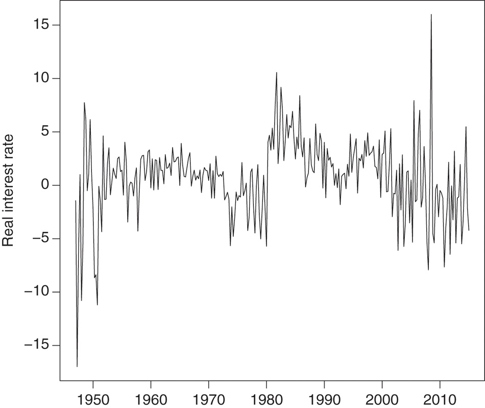
U.S. quarterly real interest rate from 1947Q1 to 2015Q1.
6.1 In-sample estimation results
We estimated the MSQAR(K, p) model by letting the number of lags vary as p = 1, 2, 3 and the number of regimes vary as K = 1, …, 5. Recall that when K = 1, the MSQAR model reduces to the linear QAR(p) with
Comparison of log marginal likelihoods.
| τ | ||||||||||
|---|---|---|---|---|---|---|---|---|---|---|
| p | 0.1 | 0.2 | 0.3 | 0.4 | 0.5 | 0.6 | 0.7 | 0.8 | 0.9 | Average |
| Panel A: QAR(p) | ||||||||||
| 1 | −820.8 | −764.2 | −730.9 | −708.2 | −694.9 | −692.6 | −700.1 | −721.4 | −760.5 | −732.6 |
| 2 | −813.7 | −764.2 | −731.9 | −715.0 | −706.6 | −705.9 | −714.1 | −732.3 | −781.7 | −740.6 |
| 3 | −792.1 | −733.2 | −704.2 | −690.5 | −684.8 | −686.3 | −698.6 | −721.7 | −770.6 | −720.2 |
| Panel B: MSQAR(2, p) | ||||||||||
| 1 | −790.5 | −732.9 | −703.6 | −690.1 | −687.8 | −693.4 | −704.8 | −731.1 | −794.3 | −725.4 |
| 2 | −781.4 | −729.3 | −703.3 | −691.5 | −690.5 | −696.8 | −710.8 | −741.1 | −808.1 | −728.1 |
| 3 | −773.5 | −724.5 | −696.9 | −683.2 | −679.9 | −685.3 | −699.6 | −728.0 | −784.5 | −717.3 |
| Panel C: MSQAR(3, p) | ||||||||||
| 1 | −807.1 | −744.5 | −711.4 | −695.5 | −690.2 | −692.5 | −701.5 | −716.3 | −755.1 | −723.8 |
| 2 | −775.4 | −720.9 | −695.8 | −684.2 | −680.9 | −683.8 | −693.3 | −709.8 | −744.5 | −709.8 |
| 3 | −766.2 | −714.4 | −688.7 | −676.9 | −673.8 | −677.3 | −689.6 | −707.4 | −741.4 | −704.0 |
| Panel D: MSQAR(4, p) | ||||||||||
| 1 | −779.6 | −731.7 | −705.3 | −699.2 | −690.1 | −692.7 | −711.6 | −725.7 | −770.5 | −722.9 |
| 2 | −752.1 | −711.2 | −691.3 | −683.0 | −679.8 | −695.1 | −700.5 | −718.1 | −757.3 | −709.8 |
| 3 | −746.7 | −706.1 | −686.7 | −684.9 | −672.3 | −677.1 | −693.4 | −716.9 | −758.2 | −704.7 |
| Panel E: MSQAR(5, p) | ||||||||||
| 1 | −777.7 | −732.8 | −715.3 | −687.8 | −688.9 | −699.8 | −701.9 | −736.3 | −765.7 | −722.9 |
| 2 | −792.5 | −734.2 | −707.3 | −686.0 | −677.4 | −689.6 | −710.9 | −729.4 | −775.9 | −722.6 |
| 3 | −744.2 | −707.1 | −693.1 | −685.3 | −672.7 | −691.3 | −689.9 | −720.6 | −758.4 | −707.0 |
For each probability level τ, this table reports the log marginal likelihood values attained by the MSQAR(K, p) specification with number of regimes equal to K = 1, 2, 3 and number of lags equal to p = 1, 2, 3. Recall that the QAR(p) corresponds to the MSQAR(1, p). The last column reports the log marginal likelihood averaged across values of τ.
Table 8 presents the posterior inference results for the unconstrained MSQAR(3, 3) models. For each model at quantile level τ, the table reports the posterior mean for each parameter, along with the corresponding numerical standard error (NSE) and the value of the Geweke (1992) test statistic. If the output of the Markov chain is compatible with stationarity, then this statistic follows a standard normal distribution. The generally insignificant values in Table 8 indicate that convergence to the stationary distribution was achieved. The estimated transition probabilities are seen to vary slightly as τ ranges from 0.1 to 0.9. From Table 7 we see that the MSQAR(3, 3) at τ = 0.5 is the best model (with a log marginal likelihood of −673.8) and the corresponding estimates of the state transition probabilities can be read from Table 8. So the posterior state classification (shown in Figure 2) and our stepwise re-estimation procedure proceeded with τi* = 0.5.
Posterior inference results: unconstrained MSQAR(3, 3) models.
| μ1 | μ2 | μ3 | δ | ϕ1 | ϕ2 | ϕ3 | p11 | p21 | p31 | p12 | p22 | p32 | |
|---|---|---|---|---|---|---|---|---|---|---|---|---|---|
| τ = 0.1 | −3.764 | 0.038 | 2.957 | 0.454 | −0.143 | −0.130 | −0.064 | 0.952 | 0.035 | 0.006 | 0.033 | 0.963 | 0.062 |
| NSE | 0.050 | 0.058 | 0.054 | 0.020 | 0.046 | 0.038 | 0.044 | 0.023 | 0.015 | 0.013 | 0.024 | 0.016 | 0.028 |
| Geweke | 0.728 | 0.340 | −0.979 | 0.250 | −0.201 | −0.241 | −0.195 | 0.374 | −1.446 | 0.985 | −0.303 | −1.403 | −0.251 |
| τ = 0.2 | −2.835 | 0.498 | 3.283 | 0.699 | −0.053 | −0.169 | 0.044 | 0.967 | 0.025 | 0.006 | 0.019 | 0.973 | 0.058 |
| NSE | 0.044 | 0.052 | 0.038 | 0.025 | 0.026 | 0.023 | 0.035 | 0.015 | 0.014 | 0.013 | 0.017 | 0.014 | 0.029 |
| Geweke | −1.066 | −0.591 | 0.724 | 0.106 | 0.615 | 0.366 | 1.421 | 0.925 | 0.054 | 0.213 | −1.043 | −0.029 | 1.283 |
| τ = 0.3 | −2.337 | 0.813 | 3.532 | 0.848 | −0.004 | −0.155 | 0.091 | 0.970 | 0.021 | 0.006 | 0.015 | 0.978 | 0.059 |
| NSE | 0.051 | 0.044 | 0.047 | 0.024 | 0.027 | 0.031 | 0.023 | 0.017 | 0.013 | 0.014 | 0.018 | 0.013 | 0.023 |
| Geweke | 0.343 | 0.777 | 0.175 | −0.318 | −0.661 | −1.573 | 0.087 | 1.004 | −0.528 | 0.459 | −1.293 | 0.984 | 0.044 |
| τ = 0.4 | −1.855 | 1.111 | 3.806 | 0.939 | 0.024 | −0.105 | 0.112 | 0.971 | 0.020 | 0.007 | 0.012 | 0.979 | 0.063 |
| NSE | 0.051 | 0.047 | 0.039 | 0.024 | 0.032 | 0.031 | 0.029 | 0.016 | 0.011 | 0.018 | 0.017 | 0.012 | 0.022 |
| Geweke | −0.284 | 0.727 | −0.669 | −1.139 | −0.382 | −1.177 | −0.922 | −0.914 | −0.121 | −0.331 | 0.442 | −0.011 | 0.418 |
| τ = 0.5 | −1.446 | 1.389 | 4.068 | 0.974 | 0.043 | −0.095 | 0.127 | 0.970 | 0.018 | 0.009 | 0.008 | 0.981 | 0.066 |
| NSE | 0.046 | 0.045 | 0.048 | 0.028 | 0.040 | 0.037 | 0.030 | 0.017 | 0.010 | 0.022 | 0.015 | 0.011 | 0.024 |
| Geweke | −0.200 | 0.920 | 1.156 | 0.617 | 0.585 | 0.326 | −0.573 | −1.123 | −0.243 | 0.968 | 0.276 | 0.223 | 0.067 |
| τ = 0.6 | −1.149 | 1.617 | 4.293 | 0.949 | 0.052 | −0.112 | 0.118 | 0.963 | 0.016 | 0.007 | 0.008 | 0.981 | 0.053 |
| NSE | 0.046 | 0.047 | 0.042 | 0.029 | 0.041 | 0.032 | 0.031 | 0.023 | 0.012 | 0.022 | 0.022 | 0.016 | 0.026 |
| Geweke | −0.531 | 0.521 | 0.254 | 0.464 | 0.010 | −0.083 | 0.696 | −0.060 | −1.694 | 0.762 | −0.808 | 1.242 | 1.272 |
| τ = 0.7 | −0.867 | 1.862 | 4.547 | 0.851 | 0.061 | −0.124 | 0.081 | 0.914 | 0.019 | 0.014 | 0.030 | 0.970 | 0.053 |
| NSE | 0.049 | 0.064 | 0.055 | 0.031 | 0.047 | 0.035 | 0.039 | 0.060 | 0.017 | 0.032 | 0.056 | 0.020 | 0.028 |
| Geweke | 1.198 | 1.413 | 0.710 | −0.910 | −0.770 | −0.867 | 0.544 | 1.225 | −1.277 | 0.694 | −1.684 | 1.119 | 0.443 |
| τ = 0.8 | −0.604 | 2.196 | 4.994 | 0.677 | 0.105 | −0.104 | 0.018 | 0.689 | 0.015 | 0.045 | 0.181 | 0.959 | 0.034 |
| NSE | 0.060 | 0.055 | 0.051 | 0.030 | 0.057 | 0.050 | 0.039 | 0.121 | 0.026 | 0.042 | 0.122 | 0.021 | 0.043 |
| Geweke | 0.842 | 0.919 | 0.554 | −0.306 | −0.889 | 1.294 | −1.506 | −0.605 | −0.032 | 1.258 | −0.177 | 0.618 | −0.543 |
| τ = 0.9 | −0.107 | 2.660 | 5.586 | 0.420 | 0.054 | −0.175 | −0.028 | 0.779 | 0.019 | 0.056 | 0.109 | 0.956 | 0.033 |
| NSE | 0.101 | 0.053 | 0.056 | 0.020 | 0.043 | 0.047 | 0.044 | 0.075 | 0.026 | 0.036 | 0.079 | 0.022 | 0.039 |
| Geweke | −0.795 | −0.721 | −0.035 | 0.072 | −0.938 | 0.725 | −0.156 | 0.077 | 0.666 | −0.179 | 0.331 | −0.415 | −0.810 |
This table reports the posterior mean of each parameter, along with the corresponding numerical standard error (NSE) and the value of the Geweke (1992) convergence statistic for the unconstrained MSQAR(3, 3) models, specified for
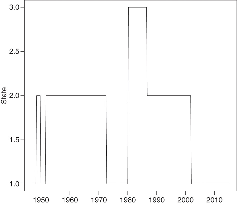
Posterior state classification obtained with the MSQAR(3, 3) model at
To economize on space we present a graphical comparison of the parameter estimates for the considered models. Figure 3 and Figure 4 correspond to the unconstrained and constrained versions of the QAR(3) models, respectively. We see immediately that both versions yield very similar point estimates (posterior means). The non-crossing restriction thus seems to hold fairly well under this linear specification. Note, however, that the reported 95% credible intervals appear differently when the non-crossing restriction is explicitly imposed. Indeed, the “bow-tie” pattern seen in Figure 4 (and Figure 6) simply reflects the fact that the stepwise re-estimation procedure conditions on more information as
Unconstrained QAR(3) model parameter estimates (posterior means) across quantile probability levels τ. The dashed lines connect the posterior means, while the shaded areas delimit the 95% credible intervals.
Non-crossing QAR(3) model parameter estimates (posterior means) across quantile probability levels τ. The dashed lines connect the posterior means, while the shaded areas delimit the 95% credible intervals.
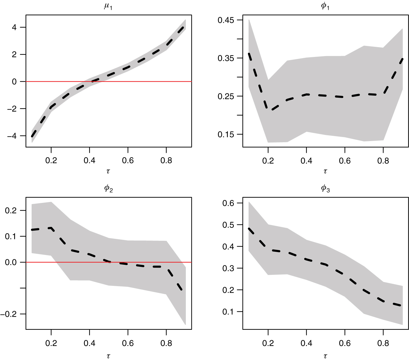
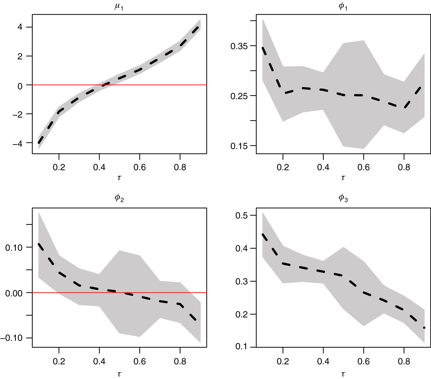
Figure 5 and Figure 6 show the estimates of μi and ϕi, i = 1, 2, 3, under the MSQAR(3, 3) specifications. In fact Figure 5 is just a graphical depiction of the information already presented in Table 8, while Figure 6 corresponds to the non-crossing version of the Markov-switching specification. We see that the estimated values of μ1, μ2, μ3 are well separated, which indicates that the regimes are well identified. The imposition of the non-crossing restriction clearly affects the estimates of the autoregressive parameters. The posterior mean estimates in Figure 5 reveal that: (i) ϕ1 generally increases with τ; (ii) ϕ2 has no clear pattern; and (iii) ϕ3 follows an inverted U-shaped pattern. On the contrary all three estimated autoregressive parameters appear more disciplined in Figure 6, each conforming more to an inverted U-shaped pattern.
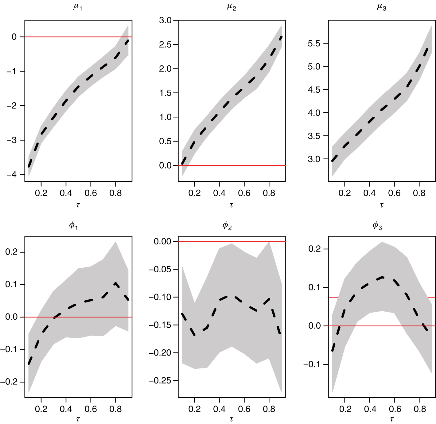
Unconstrained MSQAR(3, 3) model parameter estimates (posterior means) across quantile probability levels τ. The dashed lines connect the posterior means, while the shaded areas delimit the 95% credible intervals.
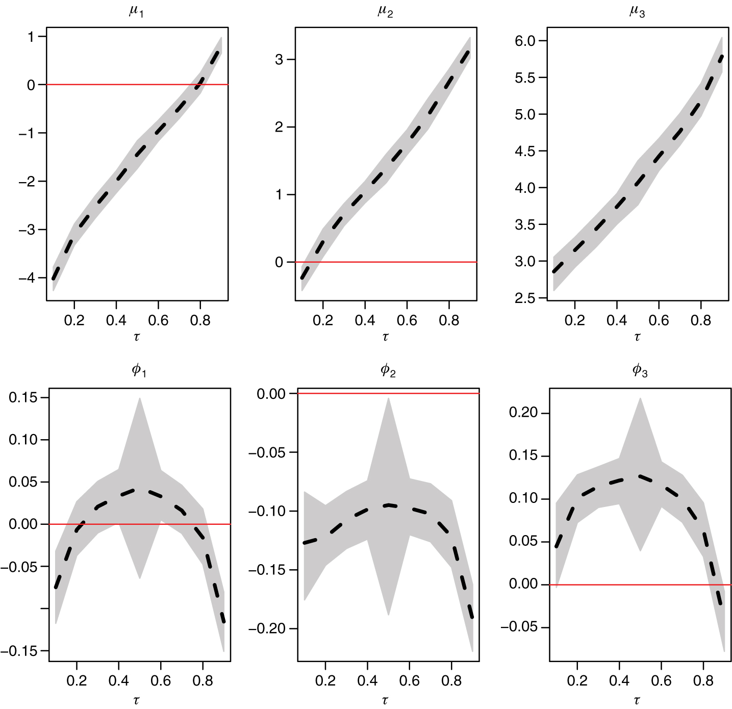
Non-crossing MSQAR(3, 3) model parameter estimates (posterior means) across quantile probability levels τ. The dashed lines connect the posterior means, while the shaded areas delimit the 95% credible intervals.
The estimation results can also be gleaned from Figure 7–Figure 10, which show the fitted quantiles for the linear QAR and the MSQAR specifications. The unconstrained quantiles are shown in Figure 7 and Figure 9, while the constrained ones are in Figure 8 and Figure 10. Although Figure 7 and Figure 8 appear quite similar, there are in fact three occurrences of crossing quantiles in Figure 7 with the QAR models: once between the quantiles at levels 0.2 and 0.3 in 2008Q1, once between the quantiles at levels 0.5 and 0.6 in 2008Q2, and once between the quantiles at levels 0.8 and 0.9 in 2008Q1. By construction, the fitted quantiles in Figure 8 have no crossings whatsoever.
Unconstrained conditional quantiles estimated with the QAR(3) models, specified for τ = 0.1, …, 0.9. The thick black line is the real interest rate series, and the light grey lines are the 9 estimated conditional quantiles from τ = 0.1 (lowest grey line) to τ = 0.9 (highest grey line).
Non-crossing conditional quantiles estimated with the QAR(3) models, specified for τ = 0.1, …, 0.9. The thick black line is the real interest rate series, and the light grey lines are the 9 estimated conditional quantiles from τ = 0.1 (lowest grey line) to τ = 0.9 (highest grey line).
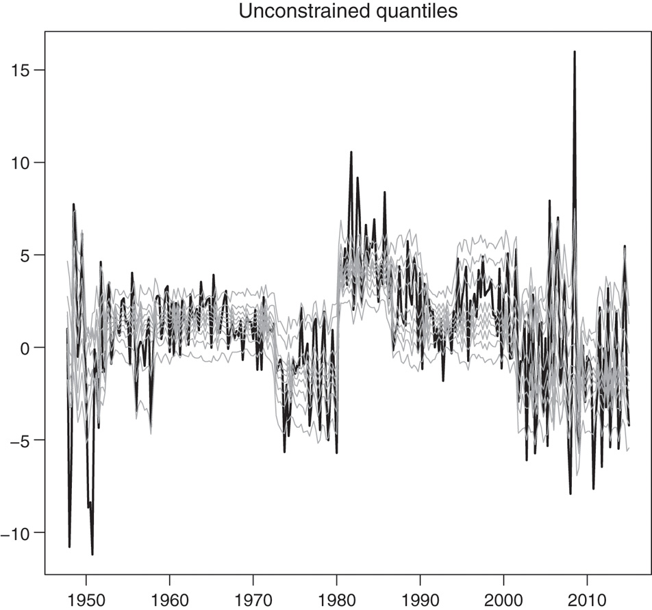
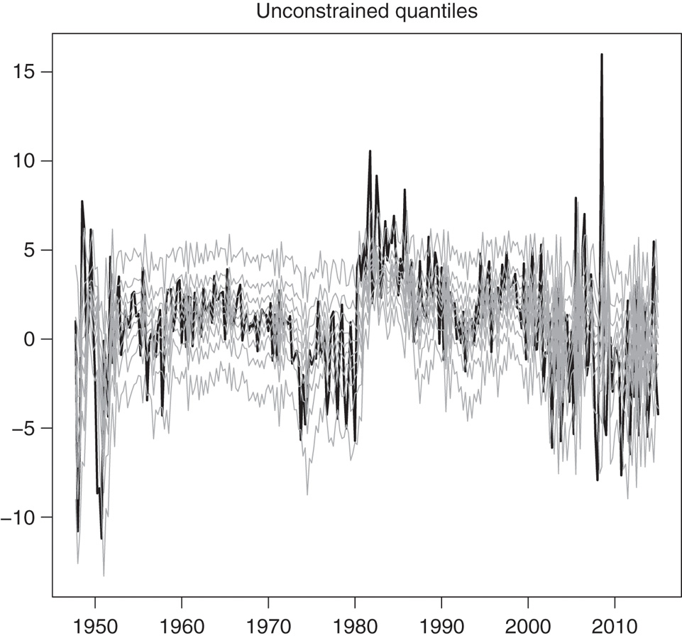
Unconstrained conditional quantiles estimated with the MSQAR(3, 3) models, specified for τ = 0.1, …, 0.9. The thick black line is the real interest rate series, and the light grey lines are the 9 estimated conditional quantiles from τ = 0.1 (lowest grey line) to τ = 0.9 (highest grey line).
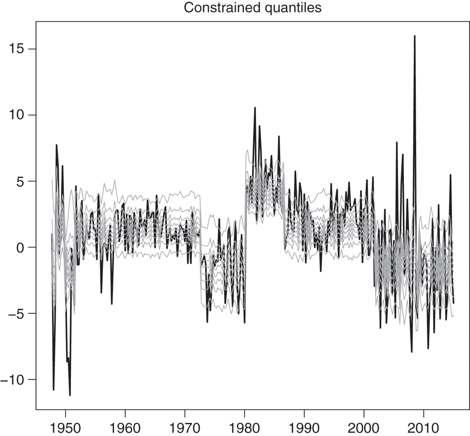
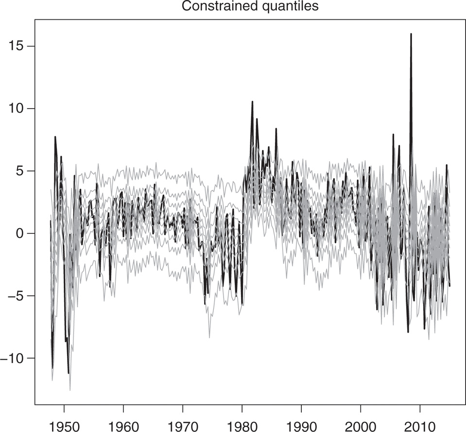
Non-crossing conditional quantiles estimated with the MSQAR(3, 3) models, specifed for τ = 0.1, …, 0.9. The thick black line is the real interest rate series, and the light grey lines are the 9 estimated conditional quantiles from τ = 0.1 (lowest grey line) to τ = 0.9 (highest grey line).
As Koenker and Xiao (2006), §4 explain, the crossing problem is potentially more acute in QAR models than in ordinary quantile regressions with exogenous covariates, since the support of the regressors is determined within the autoregressive model. So perhaps not surprisingly the estimated quantiles under the non-linear MSQAR specification cross 15 times. Among these, the most notable occurrences in Figure 9 are the 8 crossings between the quantiles at levels 0.7 and 0.8 in 1949Q2, 1949Q3, 1949Q4, 1955Q2, 1981Q3, 1989Q2, 2001Q2, and 2008Q2. Figure 10 shows the refitted MSQAR(3, 3) quantiles under the non-crossing restriction. Comparing the MSQAR quantiles in Figure 10 with the QAR quantiles in Figure 8 shows the improvements in terms of fit achieved with the non-linear specification. In line with Garcia and Perron (1996), a Markov-switching model (subject to the non-crossing quantile restriction) appears to better capture the short-term dynamics of the real interest rate.
Another interesting model assessment is a test of correct quantile specification at all quantile levels τ = 0.1, 0.2, …, 0.9, jointly. For this purpose, we use the test procedure of Escanciano and Velasco (2010). Since this test applies to both in-sample predictions and out-of-sample forecasts, we present the outcomes all together in the next section. The results (in Table 11) show the importance of imposing the non-crossing quantile restriction to achieve a correct MSQAR specification.
6.2 Out-of-sample forecasting results
In order to examine the out-of-sample forecasting performance of the MSQAR model, we used a 150-quarter rolling window over the sample period to produce one-quarter ahead forecasts. This results in 123 sets of out-of-sample quantile forecasts at levels τ = 0.1, 0.2, …, 0.9 from 1984Q3 to 2015Q1. To reduce the computational cost, we kept τi* fixed at 0.5 in the procedure for computing the predicted state classifications and the non-crossing predicted quantiles. The quantile forecasts in any given quarter were then made conditional on the prediction of the next quarter’s most likely regime.
If we let
where 𝔉t is the information set available at time t. This is the fundamental building block used to devise backtests of value-at-risk (VaR) forecasting models; see Kupiec (1995), Christoffersen (1998), Engle and Manganelli (2004), Escanciano and Velasco (2010), and Gaglianone et al. (2011). Indeed, a VaR corresponds to a conditional quantile of a financial loss distribution. Following the VaR backtesting literature, we first computed the violation rate
Table 9 reports the out-of-sample quantile violation ratios for the unconstrained and non-crossing versions of the QAR(3) and MSQAR(3, 3) models. For each model, the last column reports the average of the violation ratios across all 9 quantile levels τ. In general, we see that imposing the non-crossing restriction improves the quantile forecasts by bringing their violation ratios closer to 1. Looking at the last column, for instance, we see that the average violation ratio decreases from 1.2 to 1.174 for the QAR(3) model, and from 1.086 to 1.037 for the MSQAR(3, 3) model. Among the four specifications, the best one is clearly the MSQAR(3, 3) under the non-crossing restriction. This makes clear the value added of restricting the quantile forecasts to not cross one another in addition to allowing for Markov-switching effects. A detailed examination of Table 9 suggests that the QAR model performs well for the middle quantiles (τ = 0.5, 0.6, 0.7) while the MSQAR offers improvements for the tails of the conditional distribution.
Out-of-sample quantile violation ratios.
| τ | ||||||||||
|---|---|---|---|---|---|---|---|---|---|---|
| 0.1 | 0.2 | 0.3 | 0.4 | 0.5 | 0.6 | 0.7 | 0.8 | 0.9 | Average | |
| Panel A: Unconstrained models | ||||||||||
| QAR(3) | 1.951 | 1.504 | 1.301 | 1.138 | 1.024 | 1.003 | 0.987 | 0.965 | 0.930 | 1.200 |
| MSQAR(3, 3) | 1.382 | 1.239 | 1.165 | 0.996 | 0.959 | 1.016 | 1.034 | 1.026 | 0.958 | 1.086 |
| Panel B: Constrained models | ||||||||||
| QAR(3) | 1.951 | 1.382 | 1.219 | 1.097 | 1.024 | 1.016 | 0.964 | 0.965 | 0.949 | 1.174 |
| MSQAR(3, 3) | 1.220 | 0.989 | 1.328 | 1.077 | 0.959 | 0.967 | 0.906 | 0.915 | 0.976 | 1.037 |
This table reports the ratios
The forecasting gains were further assessed by testing their statistical significance. Table 10 reports the p-values associated with tests of the null hypothesis of a correct quantile specification at level τ. Results are reported for the unconditional coverage (UC) test of Kupiec (1995), the conditional coverage test (CC) of Christoffersen (1998), the dynamic quantile (DQ) test of Engle and Manganelli (2004) using four lags, and the quantile regression-based test for value-at-risk models (VQR) of Gaglianone et al. (2011). These tests are quite standard in the VaR forecast evaluation literature. Looking simply at the number of test outcomes that are significant at the nominal 5% level (bold entries), we see from Table 10 that the greatest benefits come when moving from the linear QAR model to the non-linear MSQAR model. Indeed there are 19 instances in which the unconstrained QAR model is rejected, while there are only 2 such instances for the unconstrained MSQAR model.
Marginal quantile specification tests: out-of-sample results.
| τ = 0.1 | τ = 0.2 | τ = 0.3 | ||||||||||
|---|---|---|---|---|---|---|---|---|---|---|---|---|
| UC | CC | DQ | VQR | UC | CC | DQ | VQR | UC | CC | DQ | VQR | |
| Panel A: Unconstrained models | ||||||||||||
| QAR(3) | 0.00 | 0.01 | 0.39 | 0.02 | 0.01 | 0.02 | 0.70 | 0.02 | 0.03 | 0.02 | 0.67 | 0.02 |
| MSQAR(3, 3) | 0.18 | 0.20 | 0.87 | 0.68 | 0.82 | 0.81 | 0.22 | 0.93 | 0.24 | 0.14 | 0.45 | 0.33 |
| Panel B: Constrained models | ||||||||||||
| QAR(3) | 0.00 | 0.00 | 0.43 | 0.00 | 0.04 | 0.06 | 0.17 | 0.11 | 0.12 | 0.03 | 0.21 | 0.27 |
| MSQAR(3, 3) | 0.43 | 0.70 | 0.15 | 0.30 | 0.33 | 0.20 | 0.77 | 0.59 | 0.24 | 0.11 | 0.40 | 0.33 |
| τ = 0.4 | τ = 0.5 | τ = 0.6 | ||||||||||
| UC | CC | DQ | VQR | UC | CC | DQ | VQR | UC | CC | DQ | VQR | |
| Panel C: Unconstrained models | ||||||||||||
| QAR(3) | 0.21 | 0.01 | 0.77 | 0.29 | 0.79 | 0.00 | 0.91 | 0.12 | 0.97 | 0.01 | 0.93 | 0.00 |
| MSQAR(3, 3) | 0.97 | 0.27 | 0.68 | 0.37 | 0.65 | 0.17 | 0.96 | 0.03 | 0.82 | 0.60 | 0.35 | 0.03 |
| Panel D: Constrained models | ||||||||||||
| QAR(3) | 0.38 | 0.14 | 0.17 | 0.72 | 0.79 | 0.00 | 0.56 | 0.12 | 0.82 | 0.01 | 0.16 | 0.00 |
| MSQAR(3, 3) | 0.49 | 0.01 | 0.78 | 0.05 | 0.65 | 0.17 | 0.21 | 0.03 | 0.29 | 0.09 | 0.11 | 0.20 |
| τ = 0.7 | τ = 0.8 | τ = 0.9 | ||||||||||
| UC | CC | DQ | VQR | UC | CC | DQ | VQR | UC | CC | DQ | VQR | |
| Panel E: Unconstrained models | ||||||||||||
| QAR(3) | 0.83 | 0.01 | 0.17 | 0.01 | 0.45 | 0.05 | 0.90 | 0.00 | 0.03 | 0.12 | 0.18 | 0.01 |
| MSQAR(3, 3) | 0.57 | 0.25 | 0.47 | 0.22 | 0.55 | 0.65 | 0.83 | 0.15 | 0.18 | 0.24 | 0.83 | 0.23 |
| Panel F: Constrained models | ||||||||||||
| QAR(3) | 0.54 | 0.04 | 0.37 | 0.01 | 0.45 | 0.04 | 0.27 | 0.00 | 0.11 | 0.18 | 0.19 | 0.01 |
| MSQAR(3, 3) | 0.23 | 0.11 | 0.14 | 0.13 | 0.71 | 0.47 | 0.25 | 0.32 | 0.43 | 0.54 | 0.90 | 0.10 |
This table reports the p-values associated with tests of a correct quantile specification at level τ. Results are reported for the unconditional coverage (UC) test of Kupiec (1995), the conditional coverage test (CC) of Christoffersen (1998), the dynamic quantile (DQ) test of Engle and Manganelli (2004), and the quantile regression-based test for value-at-risk models (VQR) of Gaglianone et al. (2011). Values < 0.01 are reported as zero and bold face entries indicate statistical significance at the nominal 5% level.
Table 11 reports the p-values associated with three versions of the Escanciano and Velasco (2010) test for correct quantile specification at all quantile levels: CvMT is based on the Cramér-von Mises functional, KT is an extended version of the Kupiec (1995) statistic, and CT is an extended version of the Christoffersen (1998) statistic. These tests are computed according to Eqs. (10), (11), and (13) in Escanciano and Velasco (2010), respectively, with the m = 9 equi-distributed points τ = 0.1, 0.2, …, 0.9 and b = 150 for their subsampling procedure. The key takeaway from Table 11 is that the MSQAR(3, 3) subject to the non-crossing restriction is the only model that passes the correct specification tests, both in and out of sample.
Joint quantile specification tests.
| In-sample results | Out-of-sample results | |||||
|---|---|---|---|---|---|---|
| CvMT | KT | CT | CvMT | KT | CT | |
| Panel A: Unconstrained models | ||||||
| QAR(3) | 0.041 | 0.187 | 0.073 | 0.000 | 0.000 | 0.000 |
| MSQAR(3, 3) | 0.911 | 0.919 | 0.106 | 0.000 | 0.000 | 0.001 |
| Panel B: Constrained models | ||||||
| QAR(3) | 0.341 | 0.000 | 0.122 | 0.000 | 0.000 | 0.000 |
| MSQAR(3, 3) | 0.740 | 0.772 | 0.642 | 0.382 | 0.244 | 0.069 |
This table reports the p-values associated with the Escanciano and Velasco (2010) test of a correct quantile specification at levels τ = 0.1, 0.2, …, 0.9, jointly. In-sample and out-of-sample results are reported using three different versions of the test: CvMT is based on the Cramér-von Mises functional, KT is an extended version of the Kupiec (1995) statistic, and CT is an extended version of the Christoffersen (1998) statistic. These tests are computed according to Eqs. (10), (11), and (13) in Escanciano and Velasco (2010), respectively. Values < 0.001 are reported here as zero and bold face entries indicate statistical significance at the nominal 5% level.
7 Conclusion
We have extended the class of linear quantile autoregression models of Koenker and Xiao (2006) by allowing for the possibility of Markov-switching regime changes à laHamilton (1989) in the conditional distribution of the response variable. We proposed a complete Bayesian methodology for: (i) estimation and inference; (ii) specification analysis of the number of regimes and the number of autoregressive lags; and (iii) enforcing the quantile monotonicity restriction that must be satisfied for any distribution to be well defined.
The Bayesian calculations are easily implemented, since all complete conditional densities used in the Gibbs sampler have closed-form expressions. As in Gelfand, Smith, and Lee (1992), Gibbs sampling is the key building block for the proposed stepwise re-estimation procedure that ensures non-crossing quantiles. Monte Carlo experiments and an illustrative empirical application show how much stronger inference and forecasting can be when the quantile monotonicity restriction is imposed.
Appendices
A Filtering and MSQAR likelihood
The likelihood function of the MSQAR model is obtained as a byproduct of the basic filter algorithm developed by Hamilton (1989) to draw probabilistic inferences about the unobserved states
Step 1. Given
where
Step 2. Compute the filtered probability as
where
The likelihood of yt appearing in the denominator of this last expression is given by
with
and where
As a byproduct of these filtering steps, the sample MSQAR likelihood function could be obtained according to
and, as Hamilton (1989) explains, rather than using
recursively for t = 2, …, p.
B Gibbs steps
In the following we shall simplify the notation and use, for example,
B.1 Sampling the state variables
In this section we describe two ways to generate draws from the distribution of s conditional upon
B.1.1 Single-move sampling
The single-move sampler proposed by Albert and Chib (1993) generates samples of s by drawing st for each t one by one from each of the following T conditional distributions:
defined for t = 1, …, T, where
The key result obtained from Bayes’ theorem for single-move sampling is:
for p + 1 ≤ t ≤ T − p + 1. Just as the Hamilton (1989) filter is started up by considering the Markov chain in isolation, we can generate the first p values of st by first obtaining a draw of s1 according to the unconditional probabilities
for t = 2, …, p. The result in (18) also needs to be slightly modified to deal with the end points. For t = T − p, …, T − 1, the draws of st are generated with probabilities:
and, when t = T, we use
With the results in (18)–(21), the normalized probabilities can be calculated as
and then drawing st is just like sampling from a multinomial distribution. Note that the state variable st is sampled iteratively for each t = 1, …, T from these discrete distributions while conditioning on the most recent draw for all other states, s−t.
B.1.2 Multi-move sampling
An alternative to the single-move sampler is the multi-move sampling approach of Carter and Kohn (1994), which draws the entire sequence s from the conditional posterior
where
Step 1. Run the Hamilton (1989) filter described in Appendix A to get
Step 2. Sample sT according to
which, as in the case of the single-move sampler, amounts to sampling a multinomial distribution.
A computational disadvantage of this approach is that it requires a run of the filtering algorithm each time a sample of state variables is generated. On the other hand, multi-move sampling may have better mixing properties than the sampler that generates the states one at a time in the case of highly correlated Markov chains (Albert & Chib, 1993; McCulloch & Tsay, 1994; Scott, 2002). In Section 5, we examine this issue in the context of the proposed MSQAR model.
B.2 Sampling the transition probabilities
Observe that upon conditioning on the sequence of state variables s, the posterior distribution of transition probabilities pij(τ) becomes independent of y and all the other model parameters. Let
where
B.3 Sampling μ ( τ ) ϕ ( τ )
Once the states have been simulated, the model can be considerably simplified by expressing it as a linear function of the parameters. Indeed, given values of s, the model in (12) can be transformed into
where
where
where
where
If we now let
where
where
with
B.4 Sampling v and δ
From (12) we see that given s,
with
where
where the GIG(ν, a, b) density is given by
with Kν(⋅) denoting a modified Bessel function of the third kind with index ν; see Dagpunar (1989) for more details and an efficient algorithm to simulate from the GIG distribution.
For the scale parameter δ we assume the usual inverse Gamma prior distribution with parameters c0/2 and d0/2, representing this here as δ ∼ IG(c0/2, d0/2). Since the joint conditional distribution of yt and vt is given as the product of the normal distribution (with mean ℓt + γvt and variance ξ2δvt) and the exponential distribution (with parameter δ), the posterior distribution of δ is propositional to
This expression is recognized as the kernel of the inverse Gamma distribution, meaning that
with c1 = c0 + 3(T − p) and
C Computation of the marginal likelihood
The first term on the right-hand side of (13) is the log of the MSQAR likelihood function in (5) evaluated at
where fN is the multivariate normal density, fIG is the inverted Gamma density, and fD is the Dirichlet density.
The log of the posterior ordinate estimate appearing as the third term on the right-hand side of (13) requires further computations. We begin with the decomposition
which is obtained by first writing the joint posterior as a product of conditional posteriors. The ordinate
which can then be estimated from the output of the Gibbs algorithm as
since
We next turn to the estimation of the ordinate
In order to obtain draws from the conditional distribution of δ, P(τ), s, v given y and
where in each of these densities we condition upon
where
This approach can be extended to obtain the estimates of the remaining ordinates in (23). Specifically, the ordinate
where
which take
where the auxiliary Gibbs draws
Upon substitution of all the estimated posterior ordinates into (23) we finally obtain from (13) the estimate of (the log of) the marginal likelihood,
References
Albert, J., and S. Chib. 1993. “Bayes Inference Via Gibbs Sampling of Autoregressive Time Series Subject to Markov Mean and Variance Shifts.” Journal of Business and Economic Statistics 11: 1–15.10.1080/07350015.1993.10509929Search in Google Scholar
Baur, D., T. Dimpfl, and R. Jung. 2012. “Stock Return Autocorrelations Revisited: A Quantile Regression Approach.” Journal of Empirical Finance 19: 254–265.10.1016/j.jempfin.2011.12.002Search in Google Scholar
Bauwens, L., A. Preminger, and J. Rombouts. 2010. “Theory and Inference for a Markov Switching GARCH Model.” Econometrics Journal 13: 218–244.10.1111/j.1368-423X.2009.00307.xSearch in Google Scholar
Billio, M., R. Casarin, and A. Osuntuyi. 2014. “Efficient Gibbs Sampling for Markov Switching GARCH Models.” Computational Statistics and Data Analysis 100: 37–57.10.1016/j.csda.2014.04.011Search in Google Scholar
Carter, C., and R. Kohn. 1994. “On Gibbs Sampling for State Space Models.” Biometrika 81: 541–553.10.1093/biomet/81.3.541Search in Google Scholar
Casella, G., and E. George. 1992. “Explaining the Gibbs Sampler.” American Statistician 46: 167–174.10.1080/00031305.1992.10475878Search in Google Scholar
Chen, C., R. Gerlach, B. Hwang, and M. McAleer. 2012. “Forecasting Value-at-Risk Using Nonlinear Regression Quantiles and the Intra-day Range.” International Journal of Forecasting 28: 557–574.10.1016/j.ijforecast.2011.12.004Search in Google Scholar
Chib, S. 1995. “Marginal Likelihood from the Gibbs Output.” Journal of the American Statistical Association 90: 1313–1321.10.1080/01621459.1995.10476635Search in Google Scholar
Chib, S. 1996. “Calculating Posterior Distributions and Modal Estimates in Markov Mixture Models.” Journal of Econometrics 75: 79–97.10.1016/0304-4076(95)01770-4Search in Google Scholar
Chow, G. 1960. “Tests of Equality Between Sets of Coefficients in Two Linear Regressions.” Econometrica 28: 591–605.10.2307/1910133Search in Google Scholar
Christoffersen, P. 1998. “Evaluating Interval Forecasts.” International Economic Review 39: 841–862.10.2307/2527341Search in Google Scholar
Dagpunar, J. 1989. “An Easily Implemented Generalized Inverse Gaussian Generator.” Communications in Statistics – Simulation and Computation 18: 703–710.10.1080/03610918908812785Search in Google Scholar
Engle, R., and S. Manganelli. 2004. “CAViaR: Conditional Autoregressive Value at Risk by Regression Quantiles.” Journal of Business and Economic Statistics 22: 367–381.10.1198/073500104000000370Search in Google Scholar
Escanciano, J., and C. Velasco. 2010. “Specification Tests of Parametric Dynamic Conditional Quantiles.” Journal of Econometrics 159: 209–221.10.1016/j.jeconom.2010.06.003Search in Google Scholar
Farcomeni, A. 2012. “Quantile Regression for Longitudinal Data Based on Latent Markov Subject-Specific Parameters.” Statistics and Computing 22: 141–152.10.1007/s11222-010-9213-0Search in Google Scholar
Ferreira, M. 2011. “Capturing Asymmetry in Real Exchange Rate with Quantile Autoregression.” Applied Economics 43: 327–340.10.1080/00036840802584919Search in Google Scholar
Frühwirth-Schnatter, S. 2001. “Markov Chain Monce Carlo Estimation of Classical and Dynamic Switching and Mixture Models.” Journal of the American Statistical Association 96: 194–209.10.1198/016214501750333063Search in Google Scholar
Frühwirth-Schnatter, S. 2006 Finite Mixture and Markov Switching Models New York, NY: Springer.Search in Google Scholar
Gaglianone, W., L. Lima, O. Linton, and D. Smith. 2011. “Evaluating Value-at-Risk Models Via Quantile Regression.” Journal of Business and Economic Statistics 29: 150–160.10.1198/jbes.2010.07318Search in Google Scholar
Galvao, A., G. Montes-Rojas, and J. Olmo. 2011. “Threshold Quantile Autoregressive Models.” Journal of Time Series Analysis 32: 253–267.10.1111/j.1467-9892.2010.00696.xSearch in Google Scholar
Galvao, A., G. Montes-Rojas, and S. Park. 2013. “Quantile Autoregressive Distributed Lag Model with an Application to House Price Returns.” Oxford Bulletin of Economics and Statistics 75: 307–321.10.1111/j.1468-0084.2011.00683.xSearch in Google Scholar
Garcia, R., and P. Perron. 1996. “An Analysis of the Real Interest Rate Under Regime Shifts.” Review of Economics and Statistics 78: 111–125.10.2307/2109851Search in Google Scholar
Gelfand, A., A. Smith, and T.-M. Lee. 1992. “Bayesian Analysis of Constrained Parameter and Truncated Data Problems Using Gibbs Sampling.” Journal of the American Statistical Association 87: 523–532.10.1080/01621459.1992.10475235Search in Google Scholar
Geraci, M., and M. Bottai. 2007. “Quantile Regression for Longitudinal Data Using the Asymmetric Laplace Distribution.” Biostatistics 8: 140–154.10.1093/biostatistics/kxj039Search in Google Scholar
Gerlach, R., C. Chen, and N. Chan. 2011. “Bayesian Time-Varying Quantile Forecasting for Value-at-Risk in Financial Markets.” Journal of Business and Economic Statistics 29: 481–492.10.1198/jbes.2010.08203Search in Google Scholar
Geweke, J. 1992. “Evaluating the Accuracy of Sampling-Based Approaches to Calculating Posterior Moments.”; In Bayesian Statistics, edited by J. Bernardo, J. Berger, A. Dawid, and A. Smith, Vol. 4 169–193. Oxford: Oxford University Press.10.21034/sr.148Search in Google Scholar
Goldfeld, S., and R. Quandt. 1973. “A Markov Model for Switching Regressions.” Journal of Econometrics 1: 3–16.10.1016/0304-4076(73)90002-XSearch in Google Scholar
Hamilton, J. 1989. “A New Approach to the Economic Analysis of Non Stationary Time Series and the Business Cycle.” Econometrica 57: 357–384.10.2307/1912559Search in Google Scholar
Kass, R., and A. Raftery. 1995. “Bayes Factors.” Journal of the American Statistical Association 90: 773–795.10.1080/01621459.1995.10476572Search in Google Scholar
Kim, C.-J., and C. Nelson. 1999 State-Space Models with Regime Switching: Classical and Gibbs-Sampling Approaches with Applications Cambridge, MA: MIT Press.10.7551/mitpress/6444.001.0001Search in Google Scholar
Koenker, R., and G. Bassett. 1978. “Regression Quantiles.” Econometrica 46: 33–49.10.2307/1913643Search in Google Scholar
Koenker, R., and J. Machado. 1999. “Goodness of Fit and Related Inference Processes for Quantile Regression.” Journal of the American Statistical Association 94: 1296–1310.10.1080/01621459.1999.10473882Search in Google Scholar
Koenker, R., and Z. Xiao. 2006. “Quantile Autoregession.” Journal of the American Statistical Association 101: 980–990.10.1198/016214506000000672Search in Google Scholar
Kottas, A., and M. Krnjajić. 2009. “Bayesian Semiparametric Modelling in Quantile Regression.” Scandinavian Journal of Statistics 36: 297–319.10.1111/j.1467-9469.2008.00626.xSearch in Google Scholar
Kotz, S., T. Kozubowski, and K. Podgórski. 2001 The Laplace Distribution and Generalizations: A Revisit with Applications to Communications, Economics, Engineering, and Finance Boston: Birkhäuser.10.1007/978-1-4612-0173-1Search in Google Scholar
Kozumi, H., and G. Kobayashi. 2011. “Gibbs Sampling Methods for Bayesian Quantile Regression.” Journal of Statistical Computation and Simulation 81: 1565–1578.10.1080/00949655.2010.496117Search in Google Scholar
Kupiec, P. 1995. “Techniques for Verifying the Accuracy of Risk Measurement Models.” Journal of Derivatives 3: 73–84.10.3905/jod.1995.407942Search in Google Scholar
Lee, C.-C., C.-F. Lee, and C.-C. Lee. 2014. “Asymmetric Dynamics in REIT Prices: Further Evidence Based on Quantile Regression Analysis.” Economic Modelling 42: 29–37.10.1016/j.econmod.2014.05.042Search in Google Scholar
Lember, J., and A. Koloydenko. 2014. “Bridging Viterbi and Posterior Decoding: A Generalized Risk Approach to Hidden Path Inference Based on Hidden Markov Models.” Journal of Machine Learning Research 15: 1–58.Search in Google Scholar
Manzan, S. 2015. “Forecasting the Distribution of Economic Variables in a Data-Rich Environment.” Journal of Business and Economic Statistics 33: 144–164.10.1080/07350015.2014.937436Search in Google Scholar
McCulloch, R., and R. Tsay. 1994. “Statistical Analysis of Economic Time Series Via Markov Switching Models.” Journal of Time Series Analysis 15: 523–539.10.1111/j.1467-9892.1994.tb00208.xSearch in Google Scholar
Piger, J. 2009. “Econometrics: Models of Regime Changes.”; In Encyclopedia of Complexity and Systems Science, edited by Robert A. Meyers, 190–202. New York, NY: Springer.10.1007/978-1-4419-7701-4_10Search in Google Scholar
Qu, Z. 2008. “Testing for Structural Change in Regression Quantiles.” Journal of Econometrics 146: 170–184.10.1016/j.jeconom.2008.08.006Search in Google Scholar
Scott, S. 2002. “Bayesian Methods for Hidden Markov Models: Recursive Computing in the 21st Century.” Journal of the American Statistical Association 97: 337–351.10.1198/016214502753479464Search in Google Scholar
Tierney, L. 1994. “Markov Chains for Exploring Posterior Distributions.” Annals of Statistics 22: 1701–1728.10.1214/aos/1176325750Search in Google Scholar
Tong, H. 1983 Threshold Models in Non-linear Time Series Analysis New York, NY: Springer-Verlag.10.1007/978-1-4684-7888-4Search in Google Scholar
Tsionas, E. 2003. “Bayesian Quantile Inference.” Journal of Statistical Computation and Simulation 9: 659–674.10.1080/0094965031000064463Search in Google Scholar
Viterbi, A. 1967. “Error Bounds for Convolutional Codes and an Asymptotically Decoding Algorithm.” IEEE Transactions on Information Theory 13: 260–269.10.1142/9789814287517_0004Search in Google Scholar
Wu, Y., and Y. Liu. 2009. “Stepwise Multiple Quantile Regression Estimation Using Non-crossing Constraints.” Statistics and its Interface 2: 299–310.10.4310/SII.2009.v2.n3.a4Search in Google Scholar
Yang, Z., A. Tu, and Y. Zeng. 2014. “Dynamic Linkages Between Asian Stock Prices and Exchange Rates: New Evidence from Causality in Quantiles.” Applied Economics 46: 1184–1201.10.1080/00036846.2013.868590Search in Google Scholar
Ye, W., Y. Zhu, Y. Wu, and B. Miao. 2016. “Markov Regime-Switching Quantile Regression Models and Financial Contagion Detection.” Insurance: Mathematics and Economics 67: 21–26.10.1016/j.insmatheco.2015.11.002Search in Google Scholar
Yu, K., and R. Moyeed. 2001. “Bayesian Quantile Regression.” Statistics and Probability Letters 54: 437–447.10.1016/S0167-7152(01)00124-9Search in Google Scholar
Yue, Y., and H. Rue. 2011. “Bayesian Inference for Additive Mixed Quantile Regression Models.” Computational Statistics and Data Analysis 55: 84–96.10.1016/j.csda.2010.05.006Search in Google Scholar
Supplemental Material
The online version of this article offers supplementary material (DOI: https://doi.org/10.1515/snde-2016-0078).
©2018 Walter de Gruyter GmbH, Berlin/Boston
Articles in the same Issue
- Markov-switching quantile autoregression: a Gibbs sampling approach
- Uncertainty in the housing market: evidence from US states
- Exchange rate misalignment and economic growth: evidence from nonlinear panel cointegration and granger causality tests
- Causal relationships between economic policy uncertainty and housing market returns in China and India: evidence from linear and nonlinear panel and time series models
- Estimation and inference of threshold regression models with measurement errors
- The spurious effect of ARCH errors on linearity tests: a theoretical note and an alternative maximum likelihood approach