A Note on Complementary Goods Mergers between Oligopolists with Market Power: Cournot Effects, Bundling and Antitrust
-
Robert T. Masson
 and
David Eisenstadt
and
David Eisenstadt

Abstract
Antitrust policy in the US and EU toward non-horizontal mergers between oligopolists is based on a strong presumption of Cournot effects and/or improvements in consumer welfare through post-merger bundling. We show that complementary goods mergers between firms that possess market power in their respective components markets do not always assure either. The analysis underscores the importance of fully specifying the nature of pre-merger rivalry among all market participants and the assumed distribution of consumer preferences when making predictions about the likely effects of such transactions.
Acknowledgments
The authors wish to express their thanks to Dr. Abigail Ferguson (Micra, Inc.); Professor Michael Waldman (Cornell University); organizers and participants of: ERC/METU VI. International Conference in Economics – Ankara, September 2002; 29th EARIE Annual Conference – Madrid, September 2002; U.S. Federal Trade Commission and Department of Justice Antitrust Division’s Joint Hearings on Health Care and Competition Law and Policy – Washington, DC, June 2003; Third Annual International Industrial Organization Conference – Atlanta, Georgia, April 2005; the 12th Annual International Industrial Organization Conference – Chicago, April 2014; Professor Francesco Parisi (University of Minnesota, University of Bologna), and anonymous referees.
Appendix
Consider one high-quality producer for each of the two components (1 and 2), denoted as 1H and 2H, that comprise a system. Also, assume the presence of at least two undifferentiated low-quality producers of these same components, denoted as 1L and 2L, respectively. Mixed systems are denoted by HL for 1H,2L and LH for 1L,2H. The “high quality system” is labeled HH for 1H,2H.
Let
Equilibrium when components are priced independently
Consider the profit maximization problem of firms 1H and 2H. Each consumer has valuations of the high-quality components denoted

Equilibrium with independent pricing of high-quality components
An angle on a circle measures one radian if the arc length is equal to the radius of the circle, r=1. So d radians can be written as
An angle on the unit circle can be written as
Differentiating with respect to
Solving eq. [6] leads to prices
Post-merger pure bundling
After the two high-quality producers merge, and in the absence of bundling, their optimal individual component prices remain the same and no CEs occur.16 If the merged firm chooses to pure bundle, consumers must purchase either a high- or low-quality system. If the pure bundle price of the high-quality system equals P, consumers who purchase it are those located on

Pure bundling of components
With pure bundling, system demand is given by17:
Based on this demand curve profits can be expressed as a function of the bundle price P. The horizontal axis starts at the price of 1 because all consumers value the high-quality system by at least this amount. Also, at a price of
Profits at the equilibrium pure bundle price are equal to 1, which are higher than the merged firm’s profits of 0.7144 under unbundled pricing. Consumer surplus is calculated as
Post-merger: mixed bundling
Mixed bundling is more profitable than pure bundling. Figure 2 shows that with a pure bundle price in excess of 1 (in the figure the pure bundle price depicted is 1.2) two “extreme” groups of consumers do not purchase the bundle. They are those who place a very low value on one high-quality component and a high value on the other. With pure bundling the firm charges a “low” bundle price equal to one to attract all consumers. However, because a significant number of consumers value the two high-quality components by an amount that significantly exceeds one, the potential exists for the merged firm to mixed bundle by setting a bundle price higher than one provided it can set individual component prices “close” to one and capture those consumers who place a high value on only one component.
For mixed bundling, we augment the notation by denoting the high-quality bundle price as
Lemma: Under mixed bundling for a given bundle price, the merged firm will choose component prices so that consumers not purchasing the bundle purchase one of the two high-quality components.
Proof: Intuitively obvious, formal proof available upon request.
The Lemma implies that given a bundled system price the stand-alone price for each component is determined by the intersection of the bundle price line and
Profits under mixed bundling are 1.1389, 13.89% higher than profits with pure bundling (and 59.4% higher than pre-merger profits). Hence, mixed bundling strictly dominates pure bundling as a post-merger pricing strategy. Consumer welfare is 0.0857, significantly lower than the pre-merger consumer welfare of 0.2508.
Welfare comparison
Since the merged firm will choose to mixed bundle, the welfare effects of the merger are derived assuming this strategy.
The 90.46% of consumers who purchased mixed systems pre-merger drops by about 60% to 35.30% post-merger. This means that 55.16% (90.46–35.30 = 64.70–9.54) of consumers switch from the purchase of a mixed system to the bundle.
In Figure 3 consumers above 0.96 and to the right of 0.96 purchase mixed systems post-merger at a price equal to 0.96. This represents a 47.5% increase in the price they pay for a mixed system, and their consumer surplus falls from 0.1183 to 0.0090.
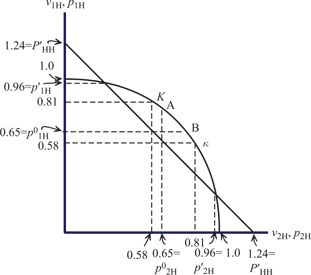
Equilibrium with mixed bundling
Consumers between A and B purchase the high-quality system both before and after. Their costs fall 5.27% from 1.3044 to 1.2356 and their consumer surplus increases from 0.0104 to 0.0169.
To calculate welfare effects for the approximately 55% switching from a hybrid system to the bundle, one must calculate their implicit price change expressed in terms of the price of the high-quality component which they bought pre-merger.
Let
In Figure 3 consumers switching from a mixed system to a high-quality system are located to the left of A and above the bundle price line and to the right of B and above the bundle price line. Some of these consumers gain from the merger while some lose. Those who gain are located on the arc between K and A and the arc between B and
Change in consumer surplus by consumer type
Table 1 in the text presents the four categories of consumers by system type, pre- versus post-merger and displays both their mass and change in their consumer surplus by type. Table 2 below is an expanded version of Table 1; it includes a formulaic calculation of consumer surplus pre- versus post-merger by category. For high-quality components, let
Pre-merger vs. post-merger consumer surplus (CS) by purchased system type and the direction of the change in CS
| Variable | Formula | Value |
| Hybrid system pre-merger | ||
| Mass | 0.353 | |
| Pre-merger CS | 0.118 | |
| Post-merger CS | 0.009 | |
| Change in CS | −0.109 | |
| Hybrid system pre-merger | ||
| Mass | 0.440 | |
| Pre-merger CS | 0.108 | |
| Post-merger CS | 0.041 | |
| Change in CS | −0.067 | |
| Hybrid system pre-merger | ||
| Mass | 0.111 | |
| Pre-merger CS | 0.014 | |
| Post-merger CS | 0.019 | |
| Change in CS | ||
| High-quality system pre-merger | ||
| Mass | 0.095 | |
| Pre-merger CS | 0.010 | |
| Post-merger CS | 0.017 | |
| Change in CS | ||
| Across all consumers | ||
| Mass | 1.000 | |
| Pre-merger CS | 0.250 | |
| Post-merger CS | 0.086 | |
| Change in CS | −0.164 | |
References
Alvisi, M., E.Carbonara, and F.Parisi. 2011. “Separating Complements: The Effects of Competition and Quality Leadership .” 103Journal of Economics.10.1007/s00712-010-0184-6Search in Google Scholar
Choi, J.P. 2008. “Mergers with Bundling in Complementary Markets ,” 56(3) The Journal of Industrial Economics553–577.10.1111/j.1467-6451.2008.00352.xSearch in Google Scholar
Cournot, A. 1838. Recherches sur Les Principes Mathématiques De La Théorie Des Richesses. Paris: Chez L. Hachette; in translation: Mathematical Principles of the Theory of Wealth, Augustus M. Kelley, New York (1971).Search in Google Scholar
Dari-Mattiacci, G., and F.Parisi. 2006. “Substituting Complements ,” 2(3) Journal of Competition Law and Economics333–347.10.1093/joclec/nhl018Search in Google Scholar
Denicolo, V. 2000. “Compatibility and Bundling with Generalist and Specialist Firms ,” 48(2) The Journal of Industrial Economics177–188.10.1111/1467-6451.00117Search in Google Scholar
Economides, N., and S.Salop. 1992. “Competition and Integration Among Complements, and Network Market Structure ,” 40(1) Journal of Industrial Economics105–123.10.2307/2950629Search in Google Scholar
Einhorn Michael, A. 1992. “Mix and Match Compatibility with Vertical Product Dimensions ,” 23(4) The RAND Journal of Economics535–547.Search in Google Scholar
Matutes, C., and P.Regibeau. 1988. “Mix and Match: Product Compatibility Without Network Externalities ,” 19(2) RAND Journal of Economics221–233.10.2307/2555701Search in Google Scholar
- 1
These include:
“…when there are no economies of scope, when two producers of complementary products merge they may offer a lower price for a bundle of those products because the merger solves a “double-marginalization problem… This is the so-called “Cournot effect” … is all the more likely in those instances where the merging firms had been exercising a degree of market power before the merger. U.S. Antitrust Division submission for OECD Roundtable on Portfolio Effects in Conglomerate Mergers, Range Effects: The United States Perspective (“OECD Roundtable”), October 12, 2001, p. 11. http://www.justice.gov/atr/public/international/9550.htm.
To the extent the merging parties enjoyed large market shares and market power in complementary goods, there will be a tendency for prices to decline post merger … fears that a conglomerate merger involving portfolio effects would lead to a welfare reducing type of price discrimination involving tying or bundling could be a thin reed to lean on as the sole rationale for blocking the merger. Ibid, pp. 30–31.
A firm may bundle its product with a complement in order to soften competition. Bundling in this case increases the profits of all participants in the market… An easy way to detect whether softening competition is the motivation for bundling is to look at competitors’ reactions to the bundle: If competitors are complaining about the possibility, we can be pretty sure that it is not serving to soften competition. Ibid, pp. 30–31.
To the extent a merger of complements gives the merged firm the incentive to lower prices because it causes the firm to internalize the negative externalities associated with higher prices (the so-called Cournot effect), it moves prices in the right direction – toward marginal costs – enhancing allocative efficiency through the elimination of double marginalization and benefitting consumers with lower prices and increased output.” “We simply could not identify any conditions under which a conglomerate merger, unlike a horizontal or vertical merger, would likely give the merged firm the ability and incentive to raise price and restrict output. William Kolasky, [then Deputy Assistant Attorney General U.S. Department of Justice], Conglomerate Mergers and Range Effects: It’s a Long Way from Chicago to Brussels, November 9, 2001.
Improved coordination between suppliers of complementary goods is an essential aspect of efficiency. Such improved coordination not only raises the parties’ joint profits, but tends to increase overall efficiency as well through lower prices or improved quality. This externality between the parties could be better internalized by their vertical [stet] merger… OECD Policy Roundtables, Vertical Mergers, 2007, United States submission, pp. 239–248.
when producers of complementary goods are pricing independently, they will not take into account the positive effect of a drop in the price of their product on the sales of the other product. Depending on the market conditions, a merged firm may internalize this effect and may have a certain incentive to lower margins if this leads to higher overall profits (this incentive is often referred to as the “Cournot effect”). Official Journal of the European Union, October 18, 2008, paragraph 117.
- 2
In criticizing the EU’s decision to challenge the GE-Honeywell merger Hal Varian concludes that “GE-Honeywell ran afoul of 19th-century thinking.” Specifically:
[A]ntitrust authorities rightly frown on companies’ coming together to set prices, since the effect is often anticompetitive. On the other hand, if the products are highly complementary and are produced in highly concentrated industries, producers left to their own devices may set prices too high because of the “Cournot effect.” [New York Times, June 28, 2001].
- 3
Supra note 1.
- 4
The absence of CEs under our demand specifications results from pre-merger price competition between a high-quality version of a component and homogenous low-quality versions sold by multiple firms that engage in pure Bertrand pricing.
- 5
AC&P also consider the case in which each integrated firm sells one high- and one low-quality component; in this case divestiture may lead to double marginalization. Under this setup, their model predicts that double marginalization (i.e., “tragedy of the anticommons” in their terminology) will more than offset the benefits from the increase in competition.
- 6
Vertical differentiation refers to a situation where all consumers are willing to pay a premium for a particular version of a component. Horizontal differentiation means some consumers would pay a premium for one version of a component while others would pay a premium for a different version.
- 7
We skip the case of zero correlation, usually modeled as preferences for the two high-quality components distributed uniformly on a unit square. This preference distribution also leads to no CEs after a merger of the two high-quality component producers, and like case B below generates a loss of consumer surplus. Pre-merger, optimal high-quality component prices are ½, as a result, one-quarter of the population purchases each of the four system types. While a merger between the two high-quality producers followed by pure bundling does not change individual component prices, post-merger one-half of the population purchases the high-quality system while the other half purchases a system comprised of only low-quality components. The merged firm captures one-half of the consumer surplus that was earned pre-merger by the consumers that purchased a hybrid system. Both Einhorn (1992) and Matutes and Regibeau (1988) model the zero-correlation case; however, their models include at most four independent producers, each with some market power.
- 8
Although we report pre- and post-merger producer surplus, both the U.S. Horizontal Merger Guidelines (2010) and EU Non-Horizontal Merger Guidelines (2008) endorse a consumer welfare standard for evaluating transactions. (“Mergers should not be permitted to create, enhance, or entrench market power or to facilitate its exercise. A merger enhances market power if it is likely to encourage one or more firms to raise price, reduce output, diminish innovation, or otherwise harm customers as a result of diminished competitive constraints or incentives.” – DOJ, FTC Horizontal Merger Guidelines, August 2010, p. 2; “Effective competition brings benefits to consumers, such as low prices, high quality products, a wide selection of goods and services, and innovation. Through its control of mergers, the Commission prevents mergers that would be likely to deprive customers of these benefits by significantly increasing the market power of firms.” – Official Journal of the European Union, 2008/C 265/07, October 2008, paragraph 10.)
- 9
Presumably such a merger would be motivated by objectives outside of those addressed by this note.
- 10
Without suppliers of low-quality components, pre-merger each component monopolist accounts for the other’s price when setting its own. Profits for each monopoly producer would equal (1 – P/2)pi, for i=1, 2, leading to identical reaction functions pi=1 – pj/2, optimal pre-merger prices for each component of 2/3, and a system price equal to 4/3. Their combination results in CEs because the merged firm maximizes total system profit of (1 – P/2)P leading to an optimal system price of 1. This same result is obtained when low-quality component producers compete pre-merger but high- and low-quality components are incompatible.
- 11
This amount is the sum of the valuations for that consumer who values the two high-quality components equally (and maximally across all consumers) and is derived from the formula for the circle, x2 + y2 = r2 where x=y and r=1, i.e. 2x2 = 1. Solving for x results in x=0.71 and 2x=1.42.
- 12
The Appendix also shows the merged firm would not choose to pure bundle. While its profits from pure bundling exceed the sum of the two firms’ pre-merger profits and consumer welfare increases, mixed bundling generates even greater profits because it allows the firm to price-discriminate and charge a higher price to those consumers who place a large value on only one of the high-quality components.
- 13
Even though the price of the bundle under either pure or mixed bundling is less than the sum of the pre-merger component prices, this result does not reflect the presence of CEs because no pricing externalities are internalized by the merger. A necessary and sufficient condition for the presence of CEs if all components are compatible is lower post-merger prices of the two high-quality components sold only separately. In case C, separate components pricing post-merger results in prices for the two high-quality components which equal their pre-merger prices. See Appendix, footnote 16.
- 14
That is, consumers with component valuations of at least (0.5834, 0.8122) or (0.8122, 0.5834).
- 15
At component price
- 16
Recall the demand for high-quality component j is given by
- 17
Let
- 18
The formal argument as to why the post-merger pure bundling equilibrium occurs at
- 19
The profit function [8] follows from the bundle demand expression [7] and the individual expressions for the high-quality components [5]. The first term captures profits from bundle sales, and equals the product of the bundle price
- 20
Pre-merger utility is
- 21
The function
- 22
Calculated as the solution to
©2014 by Walter de Gruyter Berlin / Boston
Articles in the same Issue
- Frontmatter
- Incorporation Rules
- Bargaining with Asymmetric Dispute Costs
- A Note on Complementary Goods Mergers between Oligopolists with Market Power: Cournot Effects, Bundling and Antitrust
- Institutional Regulation of Public Provision
- Litigation with Legal Aid versus Litigation with Contingent/Conditional Fees