Magnetic particle imaging of particle dynamics in complex matrix systems

2.1 Materials/particle systems

Typical tracer nanoparticle systems optimized for magnetic resonance imaging (MRI) or magnetic particle imaging (MPI) are made of Fe₃O₄ and have a multicore structure [18], [19], [20], [21], [22]. FeraSpin™ XL is a size-selected agent derived from FeraSpin™ R produced by nanoPET Pharma GmbH (Berlin, Germany), which is characterized by mean hydrodynamic particle sizes of 50 nm ≤ d _h  ≤60 nm. The hydrodynamic mean diameter of perimag^® from micromod Partikeltechnologie GmbH (Rostock, Germany) is given with d _h  ≈ 130 nm. Both commercially available particle systems show a comparable broad size distribution. Therefore, the probability is high that a small amount of the particles have optimal magnetic properties for generating a broad harmonic response as required in MPI. However, most of the signals are the result of Néel-dominated relaxation. Thus, the influence of particle-matrix interactions on the harmonic response is small. Further, signal generation is hard to understand in detail and almost impossible to predict or model. To investigate the underlying physics of particle-matrix interactions, Brownian-dominated model systems are required. SHP-25 from Ocean NanoTech (San Diego, USA) are single-core nanoparticles with a narrow size distribution that can serve as a model system. Unfortunately, these particles show significant deviations between different production batches. Further, SHP-25 shows both Brownian and Néel contributions [23]. Although iron oxide materials are preferred for bio-compatibility reasons in medical diagnostics or therapy, tailored CoFe₂O₄ nanoparticles can be used to study the physical magnetic behavior in experimental applications [24]. Such particles were manufactured by Niklas Lucht from the working group of Dr. Birgit Hankiewicz within the priority program SPP1681 of the German Research Foundation DFG in a similar way as described in the study by Nappini et al. [25]. These particles were used in MPS viscosity experiments, which enable comparisons to experimental results of other particle systems. The main particle properties of the tracer materials used for experiments are summarized in Table 1.

Depending on the particle properties, the particles relax via two possible mechanisms: the Brownian rotation or the Néel relaxation, characterized by their specific relaxation times.

The Néel zero-field relaxation time τ _N0 and Brownian zero-field relaxation time τ _B0 can approximately be measured in magnetorelaxometry (MRX) experiments. In MRX, the net magnetic moment is aligned with a static externally applied magnetic field. After a certain time all magnetic moments are aligned and the field is switched off again. Now, the effective net magnetic moment relaxes due to the thermal energy. The relaxation process follows an exponential function m(t)∝exp(−tτ−1) with a characteristic relaxation time τ. When switching off the applied field, the single magnetic moments of the particles reorient stochastically in all spatial directions such that the net magnetic moment of the particle ensemble, which is the sum of all single magnetic moments, vanishes to zero. When relaxing via the Néel mechanism, the relaxation time τ=τN0 depends on the effective anisotropy energy density K, the particle’s core volume Vc=(1/6)πdc3 with core diameter d _c and thermal energy E _T  = k _B T including the Boltzmann constant k _B and the temperature T as well as the saturation magnetization M _s , the material-specific Gilbert damping factor α ≈ 0.1 and the gyromagnetic ratio γ=1.76×1011 rad s−1T−1 of an electron as expressed in (2).

Please note that all material-specific parameters have to be taken into account. However, for approximation purposes, prefactors of the exponential function are sometimes summarized as τ0* or τ0≈1 ns. For Néel relaxation, there is no effect from particle-matrix interactions. On the other hand, when relaxing via Brownian rotation, the zero-field relaxation time τ=τB0 further depends on the surface friction expressed via the surroundings’ viscosity η acting on the hydrodynamic volume Vh=(1/6)πdh3 with the hydrodynamic diameter d _h as described in (3).

In liquid solvents, the particles can typically relax via both mechanisms—depending on the measurement parameters. In this case, the mechanism with shorter relaxation time dominates the effective relaxation time τ _eff (cf. (4)), which can be understood as parallel arrangement of both relaxation times.

Relaxation times must always be considered carefully in dynamic excitation scenarios such as during periodical excitation in MPS or MPI measurements. Additionally, it should be noted that in modalities where the magnetic field pulls the net magnetic moment, zero-field relaxation times must be replaced by field-dependent ones. The field dependence of the relaxation times were investigated in the literature studies [26], [27], [28], [29]. The field-dependent Néel relaxation time in (5) and the Brownian field-dependent relaxation time in (6) with ξ=(mμ0H)/(kBT) being the ratio of magnetic and thermal energy significantly depend on the amplitude of the applied magnetic field strength H.

Note that τNH is only valid for static fields and with the particle’s easy axis aligned with the external field direction. In contrast to ACS, which uses small magnetic field strengths so that field dependence can be neglected, MPS and MPI require large amplitudes of the applied magnetic field to reach the saturation regime of the particles and to generate higher harmonics. Here, field dependence must explicitly be taken into account. Note that the dominating relaxation mechanism can be determined from temperature-dependent MPS measurements [23].

2.2 Temperature dependence

Magnetic particle spectroscopy (MPS) is well suited for the characterization of a particle system by means of multiparametric evaluation. Especially the variation of the excitation frequency and the sample temperature allows one to derive properties of the matrix from the acquired data. While at high excitation frequencies (>10 kHz), the Néel relaxation dominates (for MPS/MPI-typical particle types), Brownian rotation of the particles at low frequencies (≪10kHz) provides access to the local interaction of the particles with their surrounding matrix. In this context, the variation of temperature is interesting for both Newtonian ferrofluids, where the temperature dependence of the dynamic viscosity η can be described by the Arrhenius–Andrade equation [30], as well as for gel systems.

With these gels, a temperature change in the sol-gel transition area leads to a significant change in the viscous or viscoelastic properties. Therefore, parametric measurements on such systems form the basis for modeling the MPS spectra as a function of matrix interaction. In order to investigate the temperature influences during the spectral characterization of such hybrid systems, a temperature-controlled MPS system was designed and realized [31]. With the help of the new design, the sample temperature can be varied in a temperature range from −20° to 120 °C during the measurements.

First temperature-dependent measurements were performed on FeraSpin™ XL (nanoPET Pharma GmbH, Berlin, Germany) [31] and SHP-25 (Ocean NanoTech, San Diego, California) at an excitation frequency of f ₀ = 5 kHz and an excitation amplitude of μ0H=25 mT, as exemplary shown in Figure 3.

In the quasi-static case, which can be explained by the Langevin function, an increase in temperature leads to a decrease in the MPS signal amplitudes at higher harmonics. The opposite behavior in Figure 3 for the freeze-dried state must therefore be attributed to a significant shortening of the relaxation times. This contradiction and the complex temperature dependence of the harmonics of the suspension (crossing of harmonic curves due to Brownian- to Néel-dominated transition from lower harmonics to higher harmonics) emphasizes the importance of particle magnetization dynamics in the description of MPS and MPI signals.

For the analysis of the magnetization behavior of the magnetic nanoparticles, dynamic magnetization curves were reconstructed (Figure 4), which allow an observation outside the frequency space of the MPS spectra and enable or simplify the comparison with other measurement methods. Another powerful evaluation method is the short-time fast Fourier transform (SFFT) analysis of harmonics during variation of the temperature. Figure 5 shows the temporally resolved course of the first 21 harmonics of a diluted SHP-25 sample (10%_vol) during the phase transition of the suspension from the subcooled to the frozen state. This approach allows one to investigate the same sample in a mobile and in an immobile state. Since the new MPS can be used to investigate time-resolved temperature-dependent processes in the millisecond range, the system provides an innovative tool for investigating biologically [9], [32], [33], [34] and technically [35] relevant scenarios.

Figure 3:

Temperature-dependent MPS spectra: The two samples (two sets of curves) are Ocean NanoTech SHP-25 in suspension and in freeze-dried immobilized form. The red color coding corresponds to the warm sample. The blue one marks the cooled—but not yet frozen—sample.

Figure 4:

Temperature-dependent MPS measurement data of the Ocean NanoTech SHP-25 suspension as spectra of the harmonics (bottom left), as time derivative of the magnetization (top left), as reconstructed time-dependent magnetization curve (top right) and as reconstructed dynamic M(H) curve (bottom right). Color coding according to Figure 3.

Figure 5:

Representation of the time-resolved temperature-dependent change of the higher harmonics of a diluted Ocean NanoTech SHP-25 sample during the phase transition from subcooled suspension to the frozen state. Figure (b) shows the phase transition of each harmonic normalized to its respective starting value to emphasize the jump of the curve at the transition point marked in (a).

2.3 Viscosity dependence

Generally, typical Fe₃O₄ nanoparticle systems optimized for MPI show both Brownian and Néel relaxation whereas the Néel relaxation even dominates the signal generation. However, only the particle contribution via Brownian rotation provides information about the particles’ surrounding. To investigate the impact of Brownian contributions on the harmonic response, Brownian-dominated particles are required as a model system. CoFe₂O₄ nanoparticles can serve as such a Brownian model system and help us revealing the underlying physics. The high anisotropy energy density of CoFe₂O₄ blocks the Néel relaxation at measurement conditions (T ≈ 298 K) almost completely for the given core size, which means that the particles are thermally blocked. Thus, the net magnetic moment of the particles only aligns via Brownian relaxation when applying an external magnetic field. The coupling of Brownian relaxation to dynamic viscosity of the particles’ environment enables the investigation of the particle mobility influence. The impact of Brownian relaxation on the harmonic response was studied in the study by Draack et al. [36] in detail using a tailored CoFe₂O₄ particle system. For that, a logarithmically equidistant viscosity series was prepared. Viscosities of the samples were adjusted by water-glycerol mixtures as solvents and are listed in Table 2.

Figure 6:

Photograph of the CoFe₂O₄ sample series providing 20 logarithmically equidistant viscosity values.

Due to a trade-off between sensitivity of the inductive sensor and relaxation time of the MNP, further investigations focus on data acquired at f ₀ = 1.0 kHz and μ0Hˆ=25 mT, as exemplary shown in Figure 7. Harmonic magnitude spectra (Figure 7a) and reconstructed dynamic M(H) curves (Figure 7b) show continuous changes with increasing viscosity.

Figure 7:

Harmonic spectra (a) and dynamic magnetization curves (b) of the CoFe₂O₄ sample series measured at f ₀ = 1.0 kHz and μ0Hˆ=25 mT.

Additionally, the residual error R (blank measurement subtracted by another blank measurement) is depicted to be able to distinguish between magnetic signals and noise. Samples with small viscosities show strong magnitudes for the fundamental and higher harmonics, whereas magnitudes of samples with high viscosities drop significantly toward higher harmonics. Reconstructed dynamic M(H) curves show distinct quasi-saturated curves for small viscosities with small hystereses (phase shift due to Brownian relaxation) and elliptical shapes with pronounced hysteresis for high viscosities (particles cannot follow the field due to high friction force on the MNPs’ hydrodynamic surface).

Furthermore, each sample of the viscosity series was measured with MPS at different excitation frequencies between 500 Hz≤f0≤25.0 kHz [18], [37] and magnetic excitation field amplitudes 5mT≤μ0Hˆ≤25 mT.

Coming from an ACS perspective, the following representation of data is common: real and imaginary parts of the fundamental frequency are plotted as a function of ω=2πf0, i.e., the parameter along a curve varies in ωτ in the range of ωminτ<ωτ<ωmaxτ. Since the relaxation time τ is constant and independent of excitation frequency, we can instead fix the excitation frequency and change τ∝η along the curve to obtain the same shape of curve. One such plot, where real and imaginary parts are plotted against viscosity η, is now generated for each harmonic frequency of the MPS data. Experimental results of the viscosity series with 20 different viscosities is depicted in Figure 8. Multiparametric investigations by varying field amplitude (Figure 8a) and frequency (Figure 8b) and, e.g., fitting data to Fokker-Planck simulations enable detailed insights into matrix interactions at comparable high field strengths. However, such experimental studies require a comparably high effort of sample preparation and prior knowledge about physical particle properties by incorporating further characterization methods like ACS [36].It should be noted that the amount of change of real and imaginary parts is a measure of the sensitivity for viscosity changes. It is obvious that the shift of the whole harmonic spectrum by varying the field amplitude and excitation frequency controls the sensitive viscosity range covered by the MPS data. The fundamental (and low harmonic frequencies) is most sensitive at high viscosities, whereas the higher harmonics are more sensitive in the lower viscosity range. Unfortunately, higher harmonics are typically limited by signal-to-noise ratio. Still, evaluation of the higher harmonics (not only harmonic ratios of fifth and third harmonic magnitudes as used by other groups [6], [8], [32]) provides a very sensitive tool with respect to particle-matrix interactions.

Figure 8:

Real and imaginary parts of odd harmonics (1f ₀ to 11f ₀) as a function of sample viscosity η. Field-dependent measurements are shown in (a), frequency-dependent data is depicted in (b).

2.4 Multi-spectral MPS

In the previous two chapters, the connection between temperature or viscosity of the sample and the harmonics spectra measured in MPS was explored. Obviously, there is no simple and direct relation apparent from the data. This is especially true, if the particle system relaxes via both the Néel relaxation mechanism as well as Brownian rotation. Most particle systems typically used for MPS/MPI contain superimposed signals of both relaxation processes. Such a tracer can only be described by complex physical models, such as Fokker–Planck equations [29], [38] or a stochastic differential equation set, where the Néel relaxation is described by the Landau–Lifshitz–Gilbert equation [39] and Brownian rotation is formulated via a forced damped oscillatory motion [17]. Since these models are very difficult and time consuming to solve and in most cases the required set of particle parameters (e.g., effective core diameter, anisotropy constant, core and hydrodynamic size distributions, etc.) is not accurately known, an alternative approach is required to cope with the complexity of these particles systems. Multispectral MPS is such a method that follows an empirical approach, where the particle system is described via a set of calibration measurements. Multispectral MPS draws a parallel to multispectral MPI reconstruction using the same underlying mathematical approach. Multispectral reconstruction solves a linear system of equations Ax=b (Figure 9). Here, A is the reference (or system) matrix containing m frequency components of n reference samples, x is the concentration vector and b is the measurement vector (i.e., the harmonic spectrum). The frequency components (real and imaginary parts) are extracted from MPS raw data via the digital lock-in method using cross-correlation. Having a reference matrix A, intermediate values between the reference samples can be estimated by linear superposition, expressing the linear system of equations as inverse problem x=A−1b. There are several approaches for solving the inverse problem, e.g., Tikhonov regularization [40] or iterative algorithms like the Karczmarz method [41], [42]. Here, we use the truncated SVD (tSVD) [43], [44], where the matrix A is approximated by A=UΣV*≈UΣkV*=Ak by means of singular value decomposition (SVD), with the reduced rectangular diagonal matrix Σ _k (truncated to the k largest eigenvalues). Since the exact inverse A ⁻¹ is indeterminable due to the fact that A is nonsquare and noise-afflicted, the pseudo-inverse A ⁺ is used in its place. It is constructed from the SVD via A+=V∑k−1U*. The reconstruction result x is then calculated as:

U ^* and V ^* denote the Hermitian transpose of U and V, respectively. The concept was introduced in the study by Viereck et al. [45] to analyze particle mixtures and is applied to viscosity or temperature here. The entries of the system matrix A and measurement vector b are complex-valued, i.e., they are the complex-valued frequency components from the MPS harmonics spectra. While in most cases, the vector x is considered real-valued, i.e., a concentration (and other observable physical quantities) is real-valued, we will find it necessary to generalize x as a complex-valued vector when considering MPS data on viscous media in the upcoming section.

Figure 9:

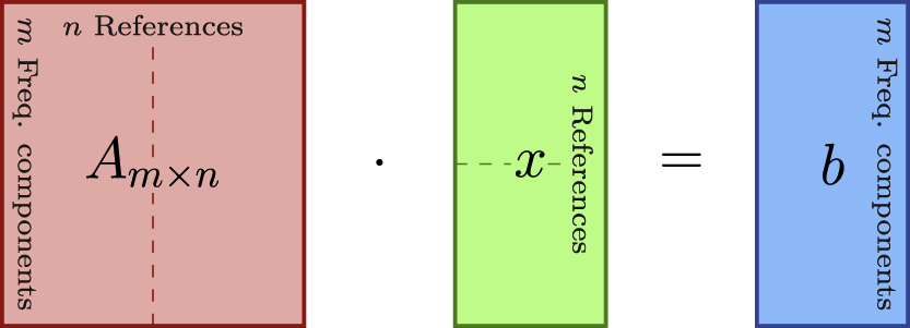
Dimensions of vectors/matrices of the linear system set of equations for the reconstruction problem. A is the system matrix, x the concentration vector and b the measurement vector or observed spectrum. The dotted lines symbolize a system with 2 references. In that case, A and x are a two-part compound matrix/vector, respectively.

The estimation of a quantity y requires calibration of at least two different references (with different y values). Measurements of intermediate states yˆ can be understood as linear superposition of the supplied references yref,i−1<yˆ<yref,i (we solve a linear set of equations in (7)). Multispectral reconstruction therefore intrinsically assumes a linear relationship between supporting reference points. Nonlinear relationships are covered by introducing mapping functions f(x)↦y from the reconstruction values x to the actual physical quantity y. Between two references, the linear mapping functions can be written in two different ways as follows:

In Sections 2.4.1 and 2.4.2, the mapping functions for MPS viscosity measurements and temperature estimation are analyzed, respectively.

2.4.1 Viscosity mapping

The continuous change of the harmonic response suggests that intermediate values between reference points can be modeled as a superposition of the references. Figure 10 shows complex-valued tSVD reconstruction results of the sample viscosity series for two reference samples. For the reconstruction using two references, the most viscous sample (M₁, dark red) and the most liquid sample (M₂₀, dark blue) were used as references. Apparently, the reconstruction results are real-valued at the two reference points. The behavior in between the reference points is more complicated. Real and imaginary parts of both references show distinct asymmetries, overshoots and especially a value ambiguity. Clearly, overshoots are more pronounced for the more viscous reference sample since the information content is reduced due to the faster decay of higher harmonics in comparison with the pure water sample. Nevertheless, a similar behavior is observed for the liquid reference sample as can be seen from the detailed excerpt shown in Figure 10b. This observation implies that a complex-valued reconstruction is required for mapping since real-valued reconstruction would be ambiguous.

Figure 10:

Spectral decomposition results of the CoFe₂O₄ viscosity series for two reference samples M₁ and M₂₀. Figure (a) shows the full value range of the reconstruction value. A detailed excerpt of small values is depicted in (b).

Adding an additional (third) reference point (M₁₁, light blue) leads to reconstruction results depicted in Figure 11.

Figure 11:

Spectral decomposition results of the CoFe₂O₄ viscosity series for three reference samples M₁, M₁₁ and M₂₀. Figure (a) shows the full value range of the reconstruction value. A detailed excerpt of small values is depicted in (b).

Again, reconstruction yields real-valued results at the reference points and overshoots in between. Evidently, a mapping function is required, which maps the reconstruction estimate x into the dynamic viscosity domain η. The complex relationship between reconstruction result xˆ and dynamic viscosity η requires a nonlinear mapping function. A viscosity mapping function using two references (as suggested in (8)) is given by

(9)ηˆ=ηref,i−[(1−xˆ)⋅(ηref,i−ηref,i−1)]

The reconstructed estimate ηˆ of the viscosity of a sample between the two reference samples depends on the viscosity values of the first reference ηref,i−1, the viscosity of the second reference η _ref,i and the reconstructed value x. Here, xˆ is either the real part Re{x}, the imaginary part Im{x} or the magnitude |x| of the reconstruction value x. Figure 12 shows estimated viscosity results for two (Figure 12a) and three (Figure 12b) references using the proposed mapping function.

Figure 12:

Viscosity mapping functions for two (a) and three (b) CoFe₂O₄ reference samples. The dashed line represents a linear mapping function between the references to illustrate the difference from the reconstruction estimate.

As can be seen from Figure 12a, the real-valued estimation Re{x} is ambiguous for higher viscosities. A mapping function using the magnitude |x| gives a unique assignment. At low viscosities, the mapping is very sensitive because the mapping function has a rapid increase of the estimated viscosity versus actual viscosity. On the other hand, the function has poor estimation resolution at the high viscosity limit. To overcome this problem, additional reference points can be consulted. Figure 12b shows the mapping function for three reference samples. The real-valued estimation is still ambivalent, although it is not as obvious as for two references due to scaling. Exact (direct) viscosity estimation is achieved at the reference points only, which is due to the modeling of the mapping function. While the direct evaluation gives inaccurate (too large) estimated viscosities, the curves obtained here can be used as calibration curves for correction. With that we can be significantly more accurate than with a “conventional” linear mapping approach. The viscosity estimation is most sensitive for viscosity values slightly larger than each reference point at which it further becomes most accurate when incorporating the nonlinear mapping relationship.

While the mapping functions in Figure 12 are obtained on a Brownian-only model system with CoFe₂O₄ particles, the same approach can be used for MPS/MPI-relevant tracers, such as FeraSpin™ XL. Figure 13 shows the viscosity mapping function for FeraSpin™ XL using real-valued reconstruction values x.

Figure 13:

Viscosity mapping function (with three references) for FeraSpin™ XL. The dashed line represents a linear mapping function between all three references to illustrate the difference from the reconstruction estimate.

Due to the strong contribution of the Néel relaxation, which does not change with viscosity, here a real-valued mapping is sufficient to create a unique function over the whole viscosity range (two orders of magnitude, starting from water). The shape of the mapping function bears strong resemblance to the mapping function of the CoFe₂O₄ sample. However, Figure 13 shows that the mapping approach is readily applicable to iron oxide particle systems used in biomedical applications.

2.4.2 Temperature mapping

Similar to the mapping function for viscosity in the previous section, we can establish a mapping function for temperature estimation Tˆ:

(10)Tˆ=Tref,i−[(1−x)⋅(Tref,i−Tref,i−1)]

Figure 14 depicts the mapping function for SHP-25 particles. The temperature estimation via tSVD of the harmonic spectrum in MPS happens to be much more linear. No oscillating behavior is observed in the decomposition, so that Figure 14 could be constructed from a real-valued reconstruction x.

Figure 14:

Temperature mapping function (with two references) for SHP-25. The dashed line represents a linear mapping function between both references to illustrate the difference from the reconstruction estimate.

A strong correlation between reconstructed values and a linear superposition (denoted by the dashed line in Figure 14) is observed for this particle system over a wide temperature range between −10° and 50 °C (with a maximum temperature deviation of approximately 10 K). For biomedical applications, e.g., cell experiments or animal studies, a much smaller range of typically 35–45 °C is needed. Arguably, multispectral MPS (or MPI) could be used directly for temperature estimation. However, with a calibrated mapping function, with references adjusted for the application’s temperature range, the estimation error for temperature can be reduced. As a general rule, the absolute estimation error can be reduced by inserting additional reference points. However, the signal-to-noise margin required for spectral decomposition poses an upper limit for the maximum number of reference points, e.g., using five reference points translates into at least five harmonics available in the measurement above the noise floor.

In conclusion, the multispectral MPS approach provides a very valuable tool for empirically treating real-world particle systems in order to use them for parameter estimation of both viscosity and temperature. Our investigations show that complex-valued reconstruction is required to estimate the particle mobility (for Brownian-dominated particle systems) due to ambiguousness of real-valued reconstruction. Since spectral decomposition in MPS is closely related to reconstruction in MPI, the findings can be transferred to mobility MPI as a quantitative medical imaging modality including information about the particles’ binding state or temperature.

3.1 Dual-frequency MPI system

Using our 2.5D field-free point (FFP) MPI scanner, the spatially resolved iron concentration of magnetic nanoparticles as well as the rheological mobility of the particles can be visualized. This method is called mobility MPI (mMPI) [46], [47], [48], [49], [50], [51], [52]. Our MPI system works with two alternative excitation frequencies (f _l  = 10 kHz and f _h  = 25 kHz), whereby an explicit gain in contrast can be recorded in mobility imaging compared to commercial MPI systems, which only provide a single excitation frequency (typically 25 kHz) [50]. Figure 15 shows the pivotal coil assembly of the MPI system built at our institute with a bore of ≤35 mm at its center.

Figure 15:

Overview of MPI system hardware.

The coil assembly contains transmit and receive coils (equivalent to the MPS system described in Section 2) as well as the NdFeB selection field generator producing the spatial encoding field for MPI imaging.

3.2 Viscosity dependence

For initial experiments, the MPI scanner was operated with a standard two-dimensional Lissajous trajectory at 25 kHz and an imaging gradient of 3 Tm⁻¹ in the isotropic imaging plane. The results show that it is possible to separate mobile (suspension) and completely immobilized particles (freeze-dried), which were acquired simultaneously in the imaging field of the scanner (Figure 16a), i.e., spatial mapping of particle mobility in MPI is possible. In order to achieve that, a multispectral reconstruction scheme [46], [48], [49], [50], [53] is employed. The reconstruction is based on the Kaczmarz method, which is considered the default algorithm in MPI [54], [55], [56]. Similar to the multispectral decomposition and reconstruction method in MPS (→ chapter 2), it relies on two or more calibration datasets being available. Multispectral reconstruction returns one image per provided reference. In Figure 16, we use two references at opposite ends of the mobility spectrum. For the final image, both reconstructed images are combined into a single false color image, where the yellow color denotes the contribution from high viscosity (freeze-dried or 100% glycerol) and green color corresponds to the low viscosity contribution (H₂O suspension).

Figure 16:

Multispectral MPI measurement results at 25 kHz depicting different mobility states of FeraSpin™ XL being separable. In (a) the particles are in H₂O suspension (left, yellow) versus freeze-dried (right, green). Figure (b) shows the tracer prepared in viscous glycerol-water mixtures with 80%vol (left) and 20%vol (right) glycerol.

Figure 16b shows the particle mobility contrast of FeraSpin™ XL in glycerol-water mixtures with 80%vol (left) and 20%vol (right) glycerol content, respectively. The samples were prepared with a particle content of 10%vol, where the rest was filled with water-glycerol mixtures of variable ratios. In Figure 16b, the spatial resolution and ability to distinguish different viscosity levels can be evaluated. Also, since the references used for reconstruction of Figure 16b, i.e., 0%vol and 100%vol glycerol, were not identical to the viscosity of the sample points, artifacts from the reconstruction (ghost images at the sides) are observed. Similar to Figure 16a, the spatial resolution depends on the particle mobility. For (partially) immobilized samples, the spatial resolution is deteriorated, which translates into the wider spot size of the sample with higher viscosity. It is still an open question, why the reconstruction (which intrinsically performs a deconvolution) is not able to equalize the different contributions in terms of apparent size (but also with respect to its estimated iron content). But it is logical to conclude that the very different signal-to-noise ratios of the two samples, i.e., smaller signal magnitude and faster decay toward higher harmonics, are responsible and not (yet) incorporated explicitly in the reconstruction process.

It should be noted that viscosity information can also be extracted by other means as discussed in the literature studies [47], [51], [57], mostly by evaluating the relaxation effects directly in the time-domain signal.

Since calibration in standard (Lissajous) 2D imaging is very time consuming, we switched to an alternative imaging scheme to be able to perform experiments on complex matrices more easily and time-efficient. In the following, we use Cartesian MPI [58], where the system employs a unidirectional excitation along the x-axis only, while the orthogonal y-direction is scanned consecutively (either by moving the sample or shifting the FFP by means of an offset field). The advantages of this method are the higher signal-to-noise ratio, which translates to a better image resolution along the trajectory axis in x-direction. Also, for evaluating the one-dimensional MPI signal, model-based or time-domain reconstruction methods can be applied.

The signal-to-noise ratio can be increased by selecting the excitation frequency of the system nearest to the expected particle response frequency. We therefore chose the lower available image frequency of 10 kHz to measure the slow relaxation of particles in the gelatin matrix. The samples were built with a visco-elastic gelatin matrix, which constitutes an application-relevant material. The matrix was prepared from 50%_vol gelatin and 50%_vol of commercial perimag^® particles, resulting in an iron concentration of 12.5  mg/mL.

The phantom (shown in Figure 17) consists of three bars, where the center bar is filled with MNP in the gelatin matrix, whereas the outer bars (left and right) are loaded with H₂O-diluted perimag^® only for reference. The gelatin matrix forms progressively over several hours, enabling MPI to observe the gelation process and its kinetics over time [59]. The gelation process is studied by Draack et al. [60], including variations in gelatin concentration, and observing reconstruction artifacts.

Figure 17:

MPI sample geometry with perimag^® particles: outer bars filled with H₂O suspension, center bar with tracer in gelatin matrix.

Figure 18 shows the MPI data measured on the phantom. Both images are recorded without any noticeable artifacts. In order to reconstruct the images, we use two different calibrations datasets as references. The image on the left was obtained on diluted perimag^® (H₂O reference); the right image on perimag^® in gelatin (gelatin reference). The two-dimensional images in the top row are displayed as surface plots to better visualize the “raw” values from the reconstructed images. As can be seen, the magnitudes depend on whether a sample point matches the calibration. For the water-filled outer bars, a higher value is observed for the H₂O reference, whereas the gelatin bar in the middle reveals a better match with the gelatin reference. X-/Y-dimensions are given in pixels on an isotropic grid (1 × 1 mm). We suggest that the mapping functions obtained from MPS (→ Section 2.4) can either be used directly in MPI or at least the same mapping approach should be applicable. However, it is still under investigation whether viscosity or temperature can be reliably quantified in MPI imaging.

Figure 18:

Viscosity in Cartesian MPI: Surface plots (upper row) and top view (lower row) of reconstructed perimag^® dash samples. Outer (left and right) dashes are filled with particles in a water suspension and center dash with particles embedded in a gelatin-water matrix. Reconstruction was performed with the water reference (left column) and with the gelatin reference (right column). X-/Y-dimensions are given in pixels. Z constitutes the ‘raw’ reconstruction value.

References

1. Gleich, B, Weizenecker, J. Tomographic imaging using the nonlinear response of magnetic particles. Nature 2005;435:1214–17. https://doi.org/10.1038/nature03808.Search in Google Scholar PubMed
2. Weizenecker, J, Gleich, B, Rahmer, J, Dahnke, H, Borgert, J. Three-dimensional real-time in vivo magnetic particle imaging. Phys Med Biol 2009;54:L1–10. https://doi.org/10.1088/0031-9155/54/5/l01.Search in Google Scholar PubMed
3. Knopp, T, Buzug, TM. Magnetic particle imaging: an introduction to imaging principles and scanner instrumentation. Heidelberg: Springer; 2012.10.1007/978-3-642-04199-0Search in Google Scholar
4. Borgert, J, Schmidt, JD, Schmale, I, Bontus, C, Gleich, B, David, B, et al.. Perspectives on clinical magnetic particle imaging. Biomedizinische Technik/Biomed Eng 2013;58:551–6. https://doi.org/10.1515/bmt-2012-0064.Search in Google Scholar PubMed
5. Biederer, S, Knopp, T, Sattel, TF, Lüdtke-Buzug, K, Gleich, B, Weizenecker, J, et al.. Magnetization response spectroscopy of superparamagnetic nanoparticles for magnetic particle imaging. J Phys Appl Phys 2009;42:205007. https://doi.org/10.1088/0022-3727/42/20/205007.Search in Google Scholar
6. Rauwerdink, AM, Giustini, AJ, Weaver, JB. Simultaneous quantification of multiple magnetic nanoparticles. Nanotechnology 2010;21:455101. https://doi.org/10.1088/0957-4484/21/45/455101.Search in Google Scholar PubMed PubMed Central
7. Rauwerdink, AM, Hansen, EW, Weaver, JB. Nanoparticle temperature estimation in combined ac and dc magnetic fields. Phys Med Biol 2009;54:L51–5. https://doi.org/10.1088/0031-9155/54/19/l01.Search in Google Scholar PubMed PubMed Central
8. Rauwerdink, AM, Weaver, JB. Viscous effects on nanoparticle magnetization harmonics. J Magn Magn Mater 2010;322:609–13. https://doi.org/10.1016/j.jmmm.2009.10.024.Search in Google Scholar
9. Rauwerdink, AM, Weaver, JB. Measurement of molecular binding using the Brownian motion of magnetic nanoparticle probes. Appl Phys Lett 2010;96:033702. https://doi.org/10.1063/1.3291063.Search in Google Scholar
10. Weaver, JB, Harding, M, Rauwerdink, AM, Hansen, EW. The effect of viscosity on the phase of the nanoparticle magnetization induced by a harmonic applied field. In: Molthen, RC, Weaver, JB, editors. Medical imaging 2010: biomedical applications in molecular, structural, and functional imaging. San Diego: SPIE; 2010. https://doi.org/10.1117/12.845576.Search in Google Scholar
11. Weaver, JB, Kuehlert, E. Measurement of magnetic nanoparticle relaxation time. Med Phys 2012;39:2765–70. https://doi.org/10.1118/1.3701775.Search in Google Scholar PubMed PubMed Central
12. Weaver, JB, Rauwerdink, AM. Chemical binding affinity estimation using MSB. In: Weaver, JB, Molthen, RC, editors. Medical imaging 2011: biomedical applications in molecular, structural, and functional imaging. Lake Buena Vista, Orlando: SPIE; 2011. https://doi.org/10.1117/12.878788.Search in Google Scholar
13. Weaver, JB, Rauwerdink, AM, Hansen, EW. Magnetic nanoparticle temperature estimation. Med Phys 2009;36:1822–9. https://doi.org/10.1118/1.3106342.Search in Google Scholar PubMed PubMed Central
14. Enpuku, K, Tsujita, Y, Nakamura, K, Sasayama, T, Yoshida, T. Biosensing utilizing magnetic markers and superconducting quantum interference devices. Supercond Sci Technol 2017;30:053002. https://doi.org/10.1088/1361-6668/aa5fce.Search in Google Scholar
15. Du, Z, Sun, Y, Higashi, O, Noguchi, Y, Enpuku, K, Draack, S, et al.. Effect of core size distribution on magnetic nanoparticle harmonics for thermometry. Jpn J Appl Phys 2019;59:010904. https://doi.org/10.7567/1347-4065/ab5c9b.https://doi.org/10.7567/1347-4065/ab5c9bSearch in Google Scholar
16. Zhong, J, Schilling, M, Ludwig, F. Magnetic nanoparticle thermometry independent of Brownian relaxation. J Phys Appl Phys 2017;51:015001. https://doi.org/10.1088/1361-6463/aa993d.Search in Google Scholar
17. Coffey, WT, Kalmykov, YP. Thermal fluctuations of magnetic nanoparticles: fifty years after brown. J Appl Phys 2012;112:121301. https://doi.org/10.1063/1.4754272.Search in Google Scholar
18. Kuhlmann, C, Khandhar, AP, Ferguson, RM, Kemp, S, Wawrzik, T, Schilling, M, et al.. Drive-field frequency dependent MPI performance of single-core magnetite nanoparticle tracers. IEEE Trans Magn 2015;51:1–4. https://doi.org/10.1109/tmag.2014.2329772.Search in Google Scholar PubMed PubMed Central
19. Ludwig, F, Eberbeck, D, Löwa, N, Steinhoff, U, Wawrzik, T, Schilling, M, et al.. Characterization of magnetic nanoparticle systems with respect to their magnetic particle imaging performance. Biomed Tech/Biomed Eng 2013;58:535–45. https://doi.org/10.1515/bmt-2013-0013.https://doi.org/10.1515/bmt-2013-0013Search in Google Scholar PubMed
20. Ludwig, F, Kuhlmann, C, Wawrzik, T, Dieckhoff, J, Lak, A, Kandhar, AP, et al.. Dynamic magnetic properties of optimized magnetic nanoparticles for magnetic particle imaging. IEEE Trans Magn 2014;50:1–4. https://doi.org/10.1109/tmag.2014.2329504.Search in Google Scholar
21. Ludwig, F, Remmer, H, Kuhlmann, C, Wawrzik, T, Arami, H, Ferguson, RM, et al.. Self-consistent magnetic properties of magnetite tracers optimized for magnetic particle imaging measured by ac susceptometry, magnetorelaxometry and magnetic particle spectroscopy. J Magn Magn Mater 2014;360:169–73. https://doi.org/10.1016/j.jmmm.2014.02.020.Search in Google Scholar PubMed PubMed Central
22. Ludwig, F, Wawrzik, T, Yoshida, T, Gehrke, N, Briel, A, Eberbeck, D, et al.. Optimization of magnetic nanoparticles for magnetic particle imaging. IEEE Trans Magn 2012;48:3780–3. https://doi.org/10.1109/tmag.2012.2197601.Search in Google Scholar
23. Draack, S, Viereck, T, Nording, F, Janssen, K-J, Schilling, M, Ludwig, F. Determination of dominating relaxation mechanisms from temperature-dependent magnetic particle spectroscopy measurements. J Magn Magn Mater 2019;474:570–3. https://doi.org/10.1016/j.jmmm.2018.11.023.Search in Google Scholar
24. Lucht, N, Friedrich, RP, Draack, S, Alexiou, C, Viereck, T, Ludwig, F, et al.. Biophysical characterization of (silica-coated) cobalt ferrite nanoparticles for hyperthermia treatment. Nanomat: Appl Mag Nanomater 2019;9:1713. https://doi.org/10.3390/nano9121713.https://doi.org/10.3390/nano9121713Search in Google Scholar PubMed PubMed Central
25. Nappini, S, Magnano, E, Bondino, F, Píš, I, Barla, A, Fantechi, E, et al.. Surface charge and coating of CoFeO nanoparticles: evidence of preserved magnetic and electronic properties. J Phys Chem C 2015;119:25529–41. https://doi.org/10.1021/acs.jpcc.5b04910.Search in Google Scholar
26. Yoshida, T, Enpuku, K. Simulation and quantitative clarification of AC susceptibility of magnetic fluid in nonlinear Brownian relaxation region. Jpn J Appl Phys 2009;48:127002. https://doi.org/10.1143/jjap.48.127002.Search in Google Scholar
27. Dieckhoff, J, Eberbeck, D, Schilling, M, Ludwig, F. Magnetic-field dependence of Brownian and Néel relaxation times. J Appl Phys 2016;119:043903. https://doi.org/10.1063/1.4940724.Search in Google Scholar
28. Coffey, WT, Cregg, PJ, Kalmykov, YUP. On the theory of Debye and Néel relaxation of single domain ferromagnetic particles. Advances in chemical physics. John Wiley & Sons, Inc.; 2007:263–464 p. https://doi.org/10.1002/9780470141410.ch5.Search in Google Scholar
29. Deissler, RJ, Wu, Y, Martens, MA. Dependence of Brownian and Néel relaxation times on magnetic field strength. Med Phys 2013;41:012301. https://doi.org/10.1118/1.4837216.Search in Google Scholar PubMed
30. Gutsalyuk, VM, Guly, IS, Mel’nichenko, YB, Klepko, VV, Vasil’ev, GI, Avdeev, NN. Mutual diffusion in aqueous gel solutions. Polym Int 1994;33:359–65. https://doi.org/10.1002/pi.1994.210330403.Search in Google Scholar
31. Draack, S, Viereck, T, Kuhlmann, C, Schilling, M, Ludwig, F. Temperature-dependent MPS measurements. Int J Mag Part Imag 2017;3. https://doi.org/10.18416/ijmpi.2017.1703018.https://doi.org/10.18416/ijmpi.2017.1703018Search in Google Scholar
32. Löwa, N, Seidel, M, Radon, P, Wiekhorst, F. Magnetic nanoparticles in different biological environments analyzed by magnetic particle spectroscopy. J Magn Magn Mater 2017;427:133–8. https://doi.org/10.1016/j.jmmm.2016.10.096.Search in Google Scholar
33. Engelmann, UM, Buhl, EM, Draack, S, Viereck, T, Ludwig, F, Schmitz-Rode, T, et al.. Magnetic relaxation of agglomerated and immobilized iron oxide nanoparticles for hyperthermia and imaging applications. IEEE Mag Lett 2018;9:1–5. https://doi.org/10.1109/lmag.2018.2879034.Search in Google Scholar
34. Poller, WC, Löwa, N, Wiekhorst, F, Taupitz, M, Wagner, S, Möller, K, et al.. Magnetic particle spectroscopy reveals dynamic changes in the magnetic behavior of very small superparamagnetic iron oxide nanoparticles during cellular uptake and enables determination of cell-labeling efficacy. J Biomed Nanotechnol 2016;12:337–46. https://doi.org/10.1166/jbn.2016.2204.Search in Google Scholar PubMed
35. Müssig, S, Granath, T, Schembri, T, Fidler, F, Haddad, D, Hiller, K-H, et al.. Anisotropic magnetic supraparticles with a magnetic particle spectroscopy fingerprint as indicators for cold-chain breach. ACS Appl Nano Mater 2019;2:4698–702. https://doi.org/10.1021/acsanm.9b00977.Search in Google Scholar
36. Draack, S, Lucht, N, Remmer, H, Martens, M, Fischer, B, Schilling, M, et al.. Multiparametric magnetic particle spectroscopy of CoFeO nanoparticles in viscous media. J Phys Chem C 2019;123:6787–801. https://doi.org/10.1021/acs.jpcc.8b10763.Search in Google Scholar
37. Wawrzik, T, Kuhlmann, C, Remmer, H, Gehrke, N, Briel, A, Schilling, M, et al.. Effect of Brownian relaxation in frequency-dependent magnetic particle spectroscopy measurements. In: 2013 International Workshop on Magnetic Particle Imaging (IWMPI). Berkeley, CA, USA: IEEE; 2013. https://doi.org/10.1109/iwmpi.2013.6528371.Search in Google Scholar
38. Weizenecker, J. “The Fokker–Planck equation for coupled Brown–Néel-rotation. Phys Med Biol 2018;63:035004. https://doi.org/10.1088/1361-6560/aaa186.Search in Google Scholar PubMed
39. Gilbert, T. Classics in magnetics a phenomenological theory of damping in ferromagnetic materials. IEEE Trans Magn 2004;40:3443–9. https://doi.org/10.1109/tmag.2004.836740.Search in Google Scholar
40. Goncharsky, A, Stepanov, VV, Tikhonov, AN, Yagola, AG. Numerical methods for the solution of ill-posed problems. Netherlands: Springer; 1995, 325. https://doi.org/10.1007/978-94-015-8480-7.Search in Google Scholar
41. Golub, GH, von Matt, U. Tikhonov regularization for large scale problems. Self; 1997. Available from: http://citeseerx.ist.psu.edu/viewdoc/summary?doi=10.1.1.51.409.10.2307/1390722Search in Google Scholar
42. Parks, PC. S. Kaczmarz (1895–1939). Int J Contr 1993;57:1263–7. https://doi.org/10.1080/00207179308934445.Search in Google Scholar
43. Hansen, PC. The truncated SVD as a method for regularization. BIT Numer Math 1987;27:534–53. https://doi.org/10.1007/bf01937276.Search in Google Scholar
44. Fierro, RD, Golub, GH, Hansen, PC, O’Leary, DP. Regularization by truncated total least squares. SIAM J Sci Comput 1997;18:1223–41. https://doi.org/10.1137/s1064827594263837.Search in Google Scholar
45. Viereck, T, Draack, S, Schilling, M, Ludwig, F. Multi-spectral magnetic particle spectroscopy for the investigation of particle mixtures. J Magn Magn Mater 2019;475:647–51. https://doi.org/10.1016/j.jmmm.2018.11.021.Search in Google Scholar
46. Haegele, J, Vaalma, S, Panagiotopoulos, N, Barkhausen, J, Vogt, FM, Borgert, J, et al.. Multi-color magnetic particle imaging for cardiovascular interventions. Phys Med Biol 2016;61:N415–26. https://doi.org/10.1088/0031-9155/61/16/n415.Search in Google Scholar PubMed
47. Hensley, D, Goodwill, P, Croft, L, Conolly, S. Preliminary experimental x-space color MPI. In: 2015 5th International Workshop on Magnetic Particle Imaging (IWMPI). Istanbul, Turkey: IEEE; 2015. https://doi.org/10.1109/iwmpi.2015.7106993.Search in Google Scholar
48. Rahmer, J, Halkola, A, Gleich, B, Schmale, I, Borgert, J. First experimental evidence of the feasibility of multi-color magnetic particle imaging. Phys Med Biol 2015;60:1775–91. https://doi.org/10.1088/0031-9155/60/5/1775.Search in Google Scholar PubMed
49. Stehning, C, Gleich, B, Rahmer, J. Simultaneous magnetic particle imaging (MPI) and temperature mapping using multi-color MPI. Int J Mag Part Imag 2016;2:1612001. https://doi.org/10.18416/ijmpi.2016.1612001.Search in Google Scholar
50. Viereck, T, Kuhlmann, C, Draack, S, Schilling, M, Ludwig, F. Dual-frequency magnetic particle imaging of the Brownian particle contribution. J Magn Magn Mater 2017;427:156–61. https://doi.org/10.1016/j.jmmm.2016.11.003.Search in Google Scholar
51. Wawrzik, T, Kuhlmann, C, Ludwig, F, Schilling, M. Estimating particle mobility in MPI. In 2013 International Workshop on Magnetic Particle Imaging (IWMPI). IEEE; 2013. https://doi.org/10.1109/IWMPI.2013.6528372.Search in Google Scholar
52. Wawrzik, T, Ludwig, F, Schilling, M. Magnetic particle imaging: exploring particle mobility. Springer proceedings in physics. Berlin, Heidelberg: Springer; 2012, vol 140. 21–5 p. https://doi.org/10.1007/978-3-642-24133-8_4.Search in Google Scholar
53. Möddel, M, Meins, C, Dieckhoff, J, Knopp, T. Viscosity quantification using multi-contrast magnetic particle imaging. New J Phys 2018;20:083001. https://doi.org/10.1088/1367-2630/aad44b.Search in Google Scholar
54. Knopp, T, Rahmer, J, Sattel, TF, Biederer, S, Weizenecker, J, Gleich, B, et al.. Weighted iterative reconstruction for magnetic particle imaging. Phys Med Biol 2010;55:1577–89. https://doi.org/10.1088/0031-9155/55/6/003.Search in Google Scholar PubMed
55. Kluth, T, Jin, B. Enhanced reconstruction in magnetic particle imaging by whitening and randomized SVD approximation. Phys Med Biol 2019;64:125026. https://doi.org/10.1088/1361-6560/ab1a4f.Search in Google Scholar PubMed
56. Weber, A, Knopp, T. Reconstruction of the magnetic particle imaging system matrix using symmetries and compressed sensing. Adv Math Phys 2015;2015:1–9. https://doi.org/10.1155/2015/460496.Search in Google Scholar
57. Utkur, M, Muslu, Y, Saritas, EU. Relaxation-based viscosity mapping for magnetic particle imaging. Phys Med Biol 2017;62:3422–39. https://doi.org/10.1088/1361-6560/62/9/3422.Search in Google Scholar PubMed
58. Werner, F, Gdaniec, N, Knopp, T. First experimental comparison between the Cartesian and the Lissajous trajectory for magnetic particle imaging. Phys Med Biol 2017;62:3407–21. https://doi.org/10.1088/1361-6560/aa6177.Search in Google Scholar PubMed
59. Remmer, H, Roeben, E, Schmidt, AM, Schilling, M, Ludwig, F. Dynamics of magnetic nanoparticles in viscoelastic media. J Magn Magn Mater 2017;427:331–5. https://doi.org/10.1016/j.jmmm.2016.10.075.Search in Google Scholar
60. Draack, S, Schilling, M, Ludwig, F, Viereck, T. Dynamic gelation process observed in Cartesian magnetic particle imaging. J Magn Magn Mater 2020;522:167478. https://doi.org/10.1016/j.jmmm.2020.167478.Search in Google Scholar
© 2020 the author(s), published by De Gruyter, Berlin/Boston
This work is licensed under the Creative Commons Attribution-NonCommercial-NoDerivatives 4.0 International License.
Articles in the same Issue
- Frontmatter
- Review
- Changes in porphyrin’s conjugation based on synthetic and post-synthetic modifications
- Magnetic Hybrid-Materials (Odenbach)