Modeling and simulation of membrane process

Abstract
The article presents the different approaches to polymer membrane mathematical modeling. Traditional models based on experimental physicochemical correlations and balance models are presented in the first part. Quantum and molecular mechanics models are presented as they are more popular for polymer membranes in fuel cells. The initial part is enclosed by neural network models which found their use for different types of processes in polymer membranes. The second part is devoted to models of fluid dynamics. The computational fluid dynamics technique can be divided into solving of Navier-Stokes equations and into Boltzmann lattice models. Both approaches are presented focusing on membrane processes.
1 Introduction
Physical phenomena is subject to many different modeling methods. This chapter is organized to give a general view of the modeling approaches, aims, capabilities, and limitations especially for polymer membrane systems. As a preferable engineering view of the modeling task the text describes two general cases from geometric perspective, zero- and higher dimensional modeling. The traditional design approach is to use zero-dimensional description of simulated entity which is less computationally demanding. The zero-dimensional methods involve classical correlations for membrane fluxes, transmembrane pressures estimations, resistances, retentions, etc. The zero-dimensional approach also involves the microscopic-level description of the phenomena modeled, e.g. by quantum or molecular analysis where the answer obtained corresponds to some indefinite point location rather than spatial distribution of resultant variables. On the other hand, modeling performed for two- or three-dimensional geometries becomes more popular for the process systems designers due to fast development of computers and numerical algorithms. This approach is generally based on hydrodynamic level of process description. Two fundamentally different, higher dimensional methods are described in the text, the more traditional finite volume method and lattice Boltzmann method. The first is derived based on discretization of Navier–Stokes equations of flow while the second relies on Boltzmann particle distribution function, which is a multidimensional function of position and momentum of fluid ensemble.
Both methods of phenomena description, zero and higher dimensional, are important and are further discussed in details for polymer membrane systems, divided into several appropriate subtopics.
2 Zero-dimensional modeling
The zero-dimensional modeling refers to the traditional technique of simulation and design approach in which the problem stated is formulated as a lumped parameter model. This approach considers any simulated and modeled phenomena as the entity with constant parameters over space analyzed. In such a case no spatial distribution of any of the variables modeled is taken into account. This approach is used in many important areas of design when there is a need to estimate key process variables, e.g. flowrates, temperatures, concentrations, pressures, and so forth. However, there is a smooth border between zero- and higher dimensional problems as many of the correlations used in this approach contain some important sizes of simulated entity, e.g. channel length, membrane width, pores diameter, and so forth. But the approach itself is still zero dimensional due to its governing equations of lumped formulation.
2.1 Basic modeling description
The most fundamental approach considers entering and exiting masses from subjected space. The mass, energy, and/or momentum streams are balanced over analyzed entity, the process is described by appropriate constitutive relation and model is formulated typically in terms of algebraic, but sometimes also differential, equations. In the membrane systems the mass balance involved is included implicitly, during the derivation of some specified formulation. The general approach to model the porous and nonporous membranes is similar but there are some differences due to their morphology. In details the model construction is dependent mainly on the membrane filtration mode due to specific flows schemes. Two basic modes are commonly used when considering the flows arrangement, namely dead-end and cross-flow setup (Figure 1). Several prediction models have been proposed as constitutive relation for the membrane permeate flux for the aforementioned modes of filtration.
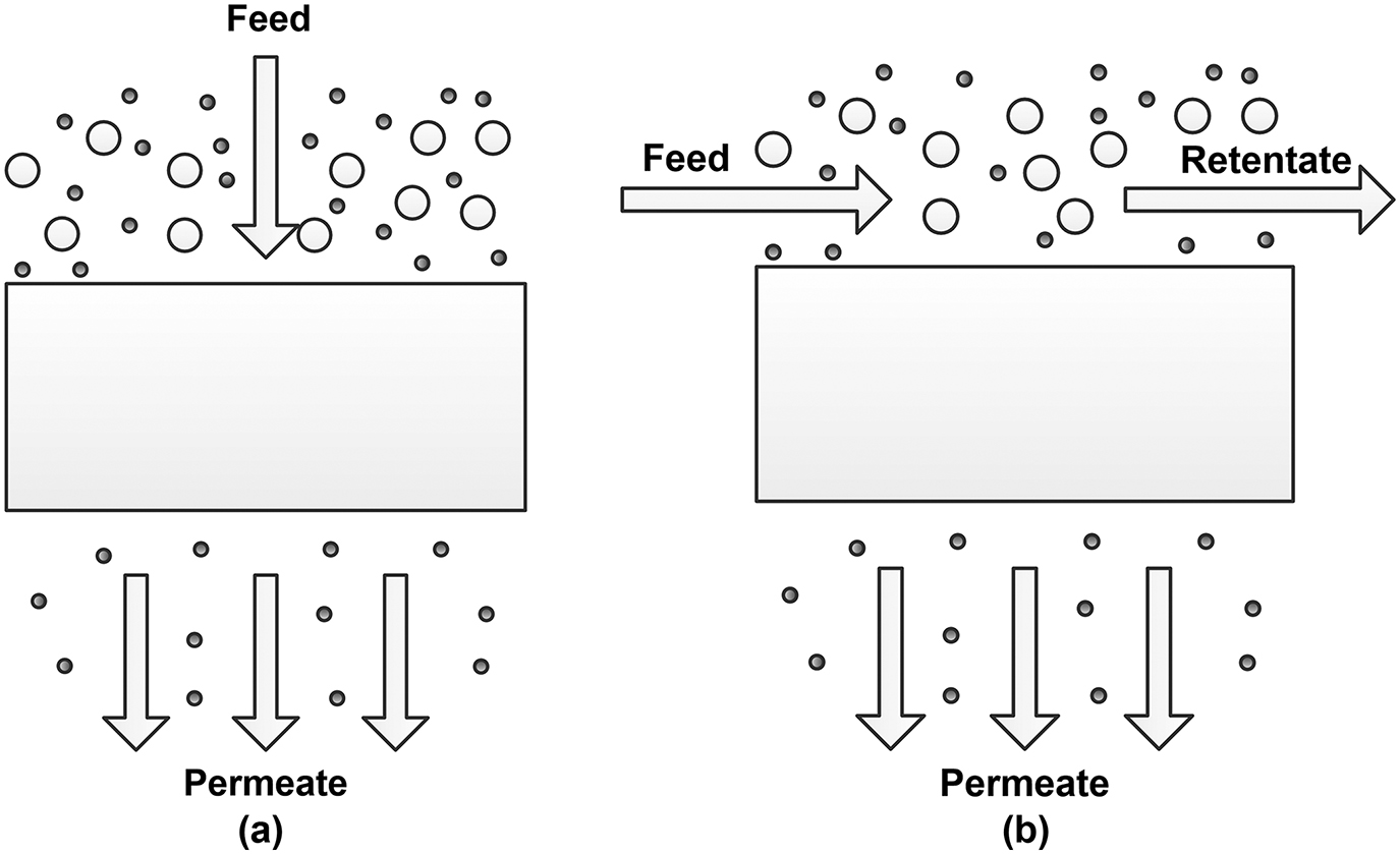
Cross-flow and dead-end membrane configuration setup.
One of the earliest approaches to the membrane transportation process is the orifice model for a pore which utilizes the Sampson [1] equation for the flow through the orifice qorifice.
where μ is the fluid viscosity and ΔP is transmembrane pressure. Applying fractional pore area Ap/Am and the pore radius r, the flux q across membrane can be obtained:
The resistance-in-series model assumes that the resistances exerted on flowing fluid by the porous media can be presented in the form of sum of resistances. The flux in the membrane filtration can be described by governing equation given as:
In the above relation q is the permeate flux with the units of velocity (discharge per unit area), ΔP is the pressure applied, Rm membrane resistance, Rpl concentration polarization (CP) layer resistance, and Rc is the cake resistance. The most problematic variable to be estimated when incorporating equation into modeling procedure is CP layer resistance. This resistance depends on amount of retained particles in layer considered and on the particle–membrane material interactions. Furthermore, the particles amount depends on the permeate flux which is then intrinsically coupled with its value so cannot be determined without prior knowing the permeate flux. It was presented [2] that pressure drop over the CP layer is constant in the case when the cake layer exists on the surface of the membrane. This pressure drop is called critical pressure ΔPc and can be determined by the relationship:
where r is the radius of the particle, NFc is the critical filtration number. NFc is the critical value of the filtration number at which the cake layer begins to appear. The filtration number NF is defined as the ratio of the energy required to transport a particle from the surface of the membrane into the bulk suspension to the thermal, dissipative energy of the particle. Details on derivation and relation of filtration number to the Einstein–Stokes equation, combined with the correction factor for high particle concentration from Hapell cell model, can be found in the literature [3].
For membrane filtration process, Darcy law (5) can also be considered as a constitutive relation. This approach formulates the flux q in terms of pressure gradient across the membrane, k permeability of the membrane, and μ fluid viscosity.
The flux q refers to the total cross section of the membrane and thus to obtain the actual average velocity u in the porous media it must be divided by the membrane porosity ϕ:
The process of filtration has the intrinsic dynamic nature. The time evolution of membrane filtration is mainly due to fouling phenomenon. Several stages of fouling are classified, and mechanisms proposed as well. The typical dynamics of the filtration resembles the flux changes during time. Initially high flux corresponds to the situation when almost pure solvent is transported across membrane. This period is characterized by short duration time and fast drop of the flux. Succeeding stage is represented by long-term gradual flux decline, and finally the last period of the process is indicated by the steady-state flux. Initial or last stage might sometimes be difficult to observe due to high rate of the process dynamics or long time of steady-state approach.
2.1.1 Standard blocking model
The model is also referred as pore blocking model. The rate of change of number of pores that are available for fluid transportation at any time of the process can be given by relation:
In the above n represents number of non-blocked pores accessible by the fluid per unit of area of the membrane surface. The variable fb is the number of pores that can be blocked by a unit volume of particles. The C0 is the initial particle concentration in the feed stream. The indices 0 refer to the initial values of specified variables. The analytical solution to the above is:
Thus two time-dependent component fluxes can be identified, the flux by unblocked pores and flux by blocked pores. The dynamics of the total flux can thus be given:
where ub0 is the flux for the blocked membrane.
2.1.2 Cake formation model
For incompressible cakes the Carman-Kozeny [4] equation relates pressure drop with velocity and membrane details:
Equation commonly used to estimate specific cake resistance rc reads:
In the above equation, μ is the viscosity of the fluid, ε is the porosity of the solid cake, Dp diameter of the particle, us superficial velocity, Φs is the sphericity of the particles in the cake. The time required for 99 % reduction of the initial flux is given by:
where cg is the particle concentration on the surface of the cake layer, c0 is the particle concentration in the bulk (feed) fluid, Rbm is the resistance of the blocked membrane and u0 is the initial velocity (to the clean surface of the membrane).
2.1.3 Physicochemical model
The model with a fouling limitation applied is given in the form that reads [5]:
where R* is the long-term fouling resistance, p, q, and r are specific constants. The variable p renders very fast initial increase in the resistance, due to the substance adsorption at the surface of the membrane which causes blocking of the pores. The q and r variables render the curvature of the time evolution of the hydraulic resistance of the membrane. R* is given by a Langmuir or Freundlich isotherms and is a function of bulk concentration and solution pH. Equation 13 represents typical correlative approach where the specific variables must be experimentally obtained for individual membrane type.
2.1.4 Reaction model
The assumption of Langmuir–Hinshelwood kinetics for the buildup of an adsorbed layer on the membrane surface [6] and leads to the description of the dynamics of its thickness l:
The Cw is the concentration of the separated substance at the membrane surface. The kinetic constants k1 and k2 refer to the rate of its deposition and removal respectively. The solution to the above reads:
The values of kinetic constants can be obtained by means of nonlinear fit numerical methods versus experimental data of cake thickness formation.
By solving classical diffusion equation of Fick’s second law, other formulation can also be given:
where ΔP is the pressure across the membrane, μ is the viscosity, p is permeability of the filtrated substance, l represents thickness of the layer, Cb bulk concentration of the substance, and Rm is the membrane resistance. The kinetic constants represented by kr and km refer to the deposition and removal process respectively. The solution to the above problem can only be done on the numerical basis.
2.1.5 Maxwell permittivity model
Gas separation by selective transport through mixed matrix polymeric membranes is commonly used technique for gaseous mixtures treatment. Chung et al. [7] suggested to use Maxwell permittivity model [8] originally aimed to predict the material resistance to external electric field. The effective permeability of composite membrane can be formulated in terms of component permeabilities of continuous Pc and dispersed phases Pd:
The above model is a simple approach that accounts for dilute suspension of spherical particles. The variable ϕd is the dispersed (polymer) phase volume fraction. Some modifications of the above approach have been proposed [9] to account for more realistic behavior. The diffusion coefficient for gas in membrane pores is then given by Knudsen diffusion coefficient that reads:
where r is the effective pore radius expressed in Å, T is the absolute temperature, MA is the molecular mass of the gas, and dg is the diameter of the gas molecules also expressed in Å. The value of the permeability of the combined sieve (Pd) and interface (Pi) void can be used along with the continuous polymer phase permeability (Pc) to obtain a predicted permeability P3MM for the three-phase mixed matrix materials by applying the Maxwell equation:
The variable ϕd is the dispersed (polymer) phase volume fraction and ϕi is the volume fraction of the interface void.
2.1.6 Modeling dense membranes
The nonporous membranes, i.e. for reverse osmosis [10], modeling shares the same principia of mass conservation as the porous, they differ in the form of constitutive relations although. The key process governing the transport through the membrane material is the solution-diffusion mechanism. The performance of the process depends on the selectivity φM of the membrane which is defined by:
where Cw and Cp are the concentration of diluted substance in the feed and permeate, respectively. The flux of permeate JP can be calculated by relationship:
where the thermodynamic function to compute a maximum value of the selectivity coefficient of the membrane reads:
In eq. 21 the variable jm is the impermeability coefficient of the membrane, and ΔPm is the operating pressure. The ω is an empirical coefficient that depends on the physical properties of the material and the operation conditions. The ΔW is the component of power of osmotic process expended for transporting ions across the membrane, T is the temperature of the fluid, and kB is the Boltzmann constant. The flow through the membrane under the operating pressure ΔPm, including impurities, depends on the hydraulic resistances of the membrane Rm and the deposit layer (cake) Rc:
where the dc and dm are the cake and membrane thicknesses, μc is the dynamic viscosity of the deposit layer.
The steady state and dynamics for dense membranes can also be modeled by considering that the driving force of the process is entirely of diffusive nature [11]. In this case the flux of specie ith is related with diffusion coefficient and specific formulation of driving force which includes corresponding permeabilities pi,perm and pi,feed difference:
where Di is the diffusion coefficient of specie ith, Si is the sorption coefficient, Hi is Henry constant, and L is the membrane thickness. The postulated dynamic description relies on variation of diffusion coefficient and permeabilities by introducing their functional forms dependent on time, Di(t) and pi,perm(t). Such mathematical simplification is valid only with assumption that diffusion coefficient is independent of diffusing specie concentration which is valid for dilute solutions. This statement is postulated by the authors [11] exclusively by particular formulation of Fick’s second law for time evolution of specie concentration in membrane material:
The initial condition for the above reads:
which formulates that no diffusing specie is contained inside the membrane in the initial moment of the process. The boundary conditions read:
that depicts that at the membrane surface (x=0) there is some initial concentration c1 of the solute, and at the downstream surface of the membrane there is a flux J(t) given by the partial pressure in the permeate channel during the process.
2.1.7 Models dependent on membrane configuration
2.1.7.1 Hollow fiber module
The hollow fiber modules are specific types of membranes in which the key constituent is their longitudinal character of the process. Starting from Fick’s diffusion law the longitudinal development of solute concentration for laminar flow is given by relation dependent on the distance z from inlet [12]:
where CA,i is the bulk concentration of specie Ath, kL is the mass transfer coefficient, d is the diameter of the fiber, uL liquid velocity. The average of the above distributed concentration Cm(z) can be obtained [13] by calculating the integral average along the z axis, to give CA:
2.1.7.2 Spiral-wound module
Spiral-wound membranes are typically used for reverse osmosis process. To estimate the concentrations in permeate following equations are proposed [14]:
where ki is the mass transfer coefficient at z location, and z is the location of feed (z=0) and outlet channel of module length L (z=L). The Jv evaluated at the same z locations is given by:
where Bs is the solute mass transfer coefficient, AW is the solvent mass transfer coefficient, Cp is the concentration of solute in the permeate, T is the temperature, R is universal gas constant, ΔP is transmembrane pressure at predefined z locations.
2.1.7.3 Capillary module
The capillary modules are commonly used for membrane distillation. The mathematical model [15] of such a unit operation must account for mass and also for heat balance equations, to enable the power requirement calculation. The formulations of equations presented below confirm also flat configuration of the membrane. The flux F expressed by the mass balance equation reads:
where rp is the pore size, ε is the porosity of the membrane, δ is the membrane thickness, τ is the pore tortuosity, Pd is the pressure at the vacuum side, Pm is the water vapor pressure at the membrane surface temperature Tm, Mw is the water molecular weight and R is the gas constant.
Heat balance equation reads:
where cp is the specific heat, Tref is the reference temperature and ΔHv the heat of vaporization of water. The model can be used to calculate the energy requirements and distillate yield flat and capillary modules.
2.1.8 Summary
The presented section outlines the broad spectrum of model approaches that are based on traditional engineers and designers techniques of membrane processes description. The modeling and the designing procedure are the tasks that employ the same tools but take different view of the process considered. The correlations presented can be used to make a simulation if some initial data like feed source, feed quality, feed/product flow, and required product quality are given. Then having selected the flow configurations and membrane elements type and setup, one can determine whether the process works as expected. The design procedure on the other hand implicates a specific results to be obtained, namely the material and geometry estimation of the membrane itself. Both views, the modeling and the design, are essentially the same regarding the theoretical and mathematical description of the process but target different needs. Most of the presented formulations are based on correlated experimental results applied to equation of mass or momentum balances. In general, the fundamental disadvantage of the models based on experimental measurements or any specific material constants obtained under particular conditions is their higher, compared to other approaches, tendency to decrease the accuracy and/or reliability when performing calculations for systems that differ significantly from systems for which they were originally established. Many correlations are designed for some specific range of temperatures, pressures, and so forth and beyond these ranges they might not be reliable source of knowledge about the system. The exception from such typical correlative issues might be to rely only on fundamental physicochemical data which do not depend on the system conditions (e.g. critical pressures, temperatures, or volumes of species involved). The mathematical approaches and models presented in next parts of this chapter address this problem because their fundamental approach is not to rely on actual, narrow range specific parameters.
2.2 Molecular modeling
Molecular modeling covers methods, algorithms, and numerical approaches which can be applied to model the molecules and atoms behavior. Its typical use is to study molecular systems varying from small to large molecular systems and material entities. The typical analysis done by molecular modeling is a phenomenon at atomistic level of the matter. In general this type of analysis can be done on the basis of molecular mechanics or quantum chemistry approach. Molecular mechanics applies laws of classical mechanics to render the interactions between atoms and molecules while quantum approach utilizes quantum theory to describe behavior of molecules, atoms, and subatomic particles. While the molecular mechanics involves atoms and bigger entities the quantum approach accounts also for electrons in the atomic structure. Both approaches are entirely different, with molecular mechanics being less accurate but faster and quantum modeling much more realistic but also with higher computational demands. There exists also approaches combined that couple the molecular and quantum mechanics in single algorithms [16] referred to as QM/MM (quantum mechanics/molecular mechanics).
2.2.1 Quantum mechanics models in polymer membranes
The underlying fundament of all quantum methods is Schrödinger equation which defines molecules in terms of interactions among nuclei and electrons and depicts geometry of the molecules by structure satisfying minimum energy requirement. The time dependent Schrödinger equation reads:
In the above the Ψ represents wave function representing quantum state of the molecule, atomic, or subatomic system. A single wave function covers at once all the particles in the system analyzed. There are many different wave functions for single system though, each of them representing appropriate description, in a chosen coordinate system. Every of the distinct representatives express all observable elements of information about the state (e.g. position, translational momentum, orbital angular momentum, spin, total angular momentum, energy). Ĥ is the Hamiltonian operator that acts on a function Ψ. The Hamiltonian corresponds to the kinetic and potential energies of a system and is the summation of all energies for every particle in the given spatial configuration at an instant time. The Schrödinger equation cannot be solved directly and approximations must be used in order to obtain results. The most commonly approximation used in order of increasing simplifications applied are as follows. The Born–Oppenheimer approximation with the assumption that the atomic nuclei do not move and only electrons kinetic energy, and the nuclei–nuclei charge interactions are accounted for. The Hartree–Fock approximation is further simplification that assumes no interaction between electrons themselves. This leads to formulation of atomic (and molecular) orbitals which can be related to stationary state of wave function for an electron in atom or molecule. The orbitals render the structure of the atom or molecule as if all the electrons formed the molecule shape without electron–electron interactions, which obviously is a simplification. The LCAO approximation (Linear Combination of Atomic Orbitals) is used in Hartree–Fock approximation to render the linear combination of atomic orbitals to further calculate the molecular orbitals by their quantum superposition. The molecular orbitals are expressed in the sense of so-called basis sets which are the linear combinations of a set of functions. The basis set is created of a finite number of orbitals, centered at each atomic nucleus within the molecule. The Hartree–Fock approximation is applicable to molecules composed from up to hundreds of atoms. Assuming no electron–electron interactions and treating every electron as independent of each other leads to overestimating of electron repulsion energy which consequently render as too high total energy of the system calculated. To overcome this problem a correlated models were proposed in which the electron correlation accounts for coupling the electrons motions that result to decrease the repulsion energy of electron–electron interactions. Lower repulsion energy estimated leads to lowering the total energy. The density functional models propose approximate correlation by an explicit term formulated on the basis of Density Functional Theory. The main assumption of this approach is the fact that the sum of the correlation energies of uniform electron cloud can be evaluated based on its density. The density functional models are usually appropriate to estimate equilibrium, geometries of transition-states, and vibrational frequencies. The density functional models reveal some serious deficiencies with regard to energetics of reaction. Due to this problem the Configuration Interaction Models were introduced in which the “auxiliary” wavefunction terms corresponding to excited states are additionally included with regards to Hartree–Fock method. The Configuration Interaction Method approaches the exact Schrodinger equation solution if the basis set applied is more complete (covers wider range of possible wavefunction states). The importance of using more complete basis sets arises due to size consistency, where typical problem is that the solution to the energy of two infinitely separated particles is not double the energy of the single particle. Due to the high demand on computing power these methods are limited to relatively small systems, however. The simplest model offering improvement over Hartree–Fock method is Moller–Plesset theory of second order (MP2). Also higher order models MP3, MP4 were formulated but they are limited to small systems. The MP2 method is practical for molecules of moderate size, although.
The basis sets mentioned earlier are functions introduced first by Slater [17] to give a description of electron orbitals. Slater type orbital (STO-xG, where x is the number of Gaussian functions) basis sets are simplest sets of Gaussian functions representing orbitals. It is significant that the same number of Gaussian functions is used to represent core and valence orbitals. They give rough estimation for orbitals but are much less computationally demanding. Pople et al. [18] formulated more complex basis sets named split valence basis sets. This formulation represents the valence orbitals by more than one basis function due to the fact that valence orbitals take main part in molecular bonding. A lot of basis sets are discussed in the references [19, 20, 21, 22, 23].
Due to the complexity of the quantum calculation it is typically not possible to perform the calculations by homebrew computer codes, instead a commercial (Gaussian, Jaguar, etc.), academic (e.g. Gamess, Firefly) or free General Public License (CP2K, PUPIL) codes are used.
Taking into account polymer membranes the main research area where the quantum modeling calculations are mostly involved are polymeric membranes in fuel cell simulations, namely proton exchange membrane fuel cell, PEMFC (Figure 2). Fuel cell is an electrochemical device that transforms the chemical energy into the electrical energy without any assistance of additional component. Principal elements of a single PEM fuel cell are: membrane, catalyst layer, gas diffusion layer (also referred to as porous transport layer), current collectors, and flow channels. Such membranes are often denoted as polymer electrolyte membranes or proton exchange membranes. The hydrogen is the fuel for the PEMFC and the hydrogen ion, proton is the charge carrier.
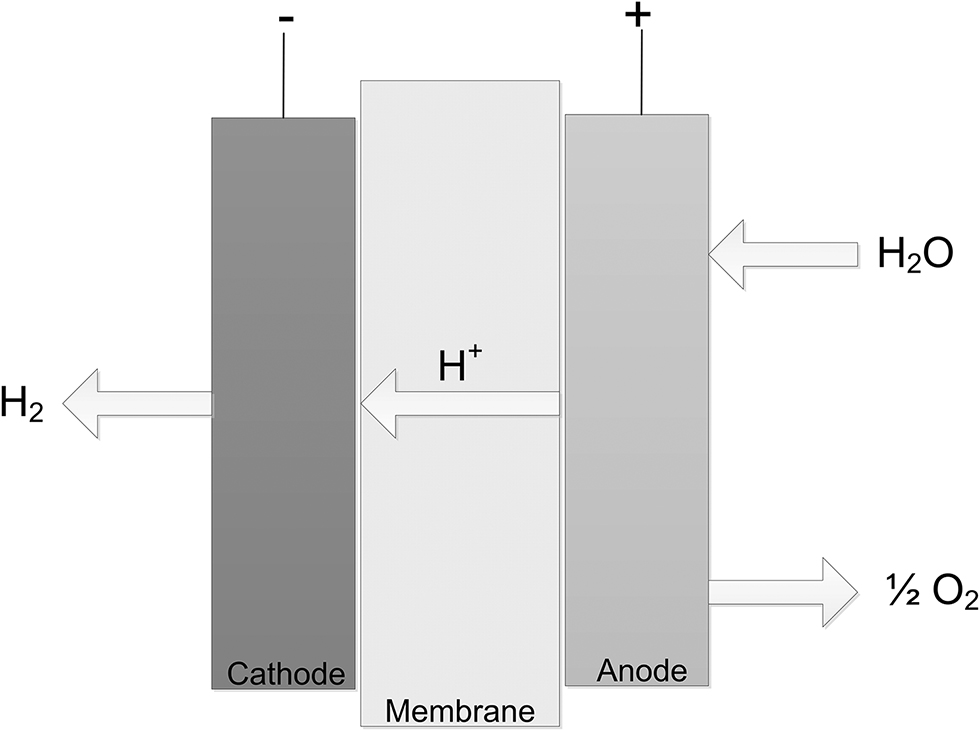
Fuel cell typical setup.
The anode reaction reads:
The cathode reaction reads:
The overall reaction is then given by stoichiometry:
The anode reaction reads:
The cathode reaction reads:
The overall reaction is then given by stoichiometry:
One of the most popular membrane material present on the market is Nafion, which is sulfonated tetrafluoroethylene based fluoropolymer-copolymer (RF[OCF2CF(CF3)2]nOCF2CF2SO3H). Nafion is most often formed as a thin foil and used as a protons transporting membrane, namely ionomer, while being a barrier for electrons or anions. This material exhibits also high thermal and chemical resistance.
Yu et al. [24, 25] simulated chemical mechanisms of degradation of Nafion using JAGUAR 7.0 code. They incorporated Density Functional Theory to formulate the potential energy surfaces for various possible reactions accounting for intermediates which could be created when Nafion is exposed to molecular hydrogen, molecular oxygen, or protons in the presence of the platinum catalyst. The B3LYP (Becke, three-parameter, Lee-Yang-Parr) exchange-correlation functional was used with 6-311G** basis set (six Gaussian primitive function for core orbitals, and a linear combination of two basis function for each valence orbitals, the stars indicate extension to the main basis set by adding double polarization functions). Based on the results three mechanisms by which OH radical species formed on a platinum surface lead to degradation of Nafion polymer were proposed and experimentally validated by F NMR and mass spectroscopy.
Sakai et al. [26] used Gaussian software commercial tool to model the deprotonation reaction of the sulfonic group (SO3H) in a hydrocarbon membrane, as a new proton conductor for polymer electrolyte membranes (PEM) of polymer electrolyte fuel cells (PEFC). Similarly as case previously described 6-311+G(d, p) basis set was used at the B3LYP density functional theory level. The difference in basis set is presented by the plus sign meaning that the diffuse function is used for p and d orbitals. The diffuse functions are of high significance for anions to describe the electrons that are at longer distances from the nuclei. The quantum model was used to investigate and simulate the behavior of the sulfonic group of sulfonic acid C6H5SO3H as a model of a hydrocarbon membrane. As the concluding statement the following two properties were noticed as the main factors decreasing proton conductivity at low hydration levels: sulfonic acid has low acidity because deprotonation of SO3H group and protonation of SO3− anion occur with the same probability; and the SO3− anion of sulfonic acid binds strongly with the H3O+ in comparison with short side chain perfluorosulfonic acid. Paddison et al. [27] presented earlier similar study using B3LYP/6-311G** level density functional theory to perform modeling of a hydrocarbon polymer membrane (CF3CF(O(CF2)2SO3H)(CF2)nCF(O(CF2)2SO3H)CF3, where n = 5, 7, and 9). The quantum simulation performed exposed that the number of water molecules needed to connect the sulfonic acid groups is a proportional function of the number of fluoromethylene groups in the main chain, with one, two, and three water molecules needed to connect the sulfonic acid groups in parts with n = 5, 7, and 9, respectively. It is also worth noting that the simulation was performed with explicit addition of water molecules to each of the polymeric fragments (an implicit approach would be to replace intermolecular interactions by so-called averaged field), which allowed to conclude that the minimum number of water molecules required to affect proton transfer also increases as the number of separating tetrafluoroethylene units in the main chain is increased. These quantum modeling calculations provided the results that might be used to evaluate the impact of changes of polymer chemistry on proton conduction, including the side chain length and acidic functional group.
There are also modeling studies which are based on approaches which in their background rely on quantum calculations. One of such approach is COSMO model (conductor-like screening model) which is used for estimating the electrostatic interaction between a molecule and a solvent. This model belongs to continuum solvation or averaged field group of models. The main concept is to approximate the solvent presence by a dielectric continuum, surrounding the molecules. The COSMO method can be used with Hartree–Fock methods or density functional theory calculations. The extensions for real solvents allow to estimate the chemical potentials of substances in liquids which consequently leads to other thermodynamic equilibrium properties (such as solubility, activity coefficients, vapor pressures, partition coefficients and free solvation energies) calculations. The example of the use of such an approach is the work of Shah et al. [28] They used a COSMO-SAC model (conductor-like screening model – segment activity coefficient) to estimate the structure–properties relationships between the polymer structure and membrane performance. The GGA/VWN-BP functional setting and the DNPv4.0.0 basis set was used. The generalized gradient approximation (GGA) takes into account variations in the density by including the gradient of the density in the functional. The Vosko-Wilk-Nusair [29] (VWN) is the correlation for many electron system of the spin-polarized homogeneous electron gas. The VWN correlation energy per particle of homogenous electron gas improves the theory and experiment agreement. The VWN-BP represents the Becke-Perdew version of the VWN functional. The model can successfully predict two component sorption from single component sorption data. The model functions poorly in the case of some polar solvent/polar polymer combinations, however.
2.2.2 Molecular mechanics models in polymer membranes
Molecular mechanics describes molecules and chemical bonds based on van der Waals and Coulombic interactions. This approach utilizes classical mechanics laws to model the molecular systems.
The molecular mechanics approach expresses the energetic state of a molecule in terms of a sum of contributions resulted from deviations from an ideal molecular state of lowest energy. The summation is taken over stretch contributions (bond distances), bend contributions (bond angles) and torsion contributions (torsion angles) of mechanical state of molecular system. Additional terms are the contributions due to van der Waals and Coulombic (non-bonded) interactions. Stretches and bends contributions of molecular bonds are formulated in terms of Hook’s law forms. Torsion contributions need to reflect the torsional potential periodicity which takes the form of trigonometric functionals that accounts for such behavior. The energy of torsion can be formulated in terms of Fourier series which allow to account for energy differences in cis and trans conformers or between planar and perpendicular conformers. The van der Waals and Coulombic interactions summation formulate the non-bonded interactions terms. Some explicit summation terms might also be included to account for such interactions as hydrogen bonding. The van der Waals interactions are formulated as a summation of attractive and repulsive components. The Coulombic term is formulated to take the charges interactions into account.
The advantage of molecular mechanics models over quantum approach is their greater ability to transfer the geometrical variables between molecules, and expectable parameters dependence on atomic hybridization. This makes the molecular mechanics approach to be easier when applying initial geometrical guess to a numerical solving procedure and allows to perform faster calculations. In practice the computational load increases linearly with the size of molecular system modeled (which is not the case for quantum mechanics). The parametrization of molecular models is also important advantage over quantum approach. On the other hand the simplicity of the molecular mechanics models imposes some limitation when comparing with quantum approach. The most important limitation is that molecular mechanics allow to represent only the equilibrium states (geometries and conformations) of the molecular systems. The parametrization of functionals describing force fields has not yet been done to comply with nonequilibrium molecular states. The next limitation is that the molecular mechanics cannot describe the electron distributions in molecules which is an important feature when simulating chemical reactions. Consequently, the underlying principal nature of molecular mechanics modeling is its approximation character, for which the accuracy depends on quality of the parameters used and on the classifications of relations between molecules. This is typical that for such an approach going beyond the range of parametrizations, i.e. describing some new molecular structures, is expected to be burdened with high and difficult to estimate error.
The extension to molecular mechanics approach is molecular dynamics, which besides of the molecular mechanics interactions, consist on solving, typically on numerical basis, the classical equations of motion. After the calculation of potential energy field, the forces acting on the molecules are computed. Applying the Newton’s equations of motions to the molecular system results in a molecular momenta estimation which consequently leads to movement patterns of molecules. Such a system of differential equations is solved using specified step-by-step numerical algorithm of integration. The differential equations set is typically characterized by high stiffness (relation of fast to slow dynamic components of the process simulated) and special numerical treatment is needed. Historically the Gear’s algorithm [30] was designed for such systems, which is the two step method assembled of explicit Adams and implicit backward differentiation formula. Recently Verlet algorithm [31] is used to solve this problem, which is purposely designed to integrate the equations of motion.
As an example the effects of molecular structure on the polymer membrane process is studied by means of molecular mechanics calculations by Shen et al. [32] The molecular mechanics models require to input initial structure of the modeled molecular system. For the polymers a heuristic method [33] can be used, which consist on building the structure from monomers and locating them randomly in computational space. Authors examined the rejection mechanisms for contaminants in polyamide reverse osmosis process and based on the molecular dynamics calculations concluded that the solute rejection is positively correlated with the Van der Waals size of the dehydrated solutes due to decreasing accessible intermolecular volume between polymer chains of the membrane with solute size. Devanathan et al. [34] performed an ab initio study (from first principles) of proton transport in Nafion polymer membrane. One of the most fundamental problems in proton transport is that it does not follow diffusive transport of water molecules but make use of surrounding hydrogen bonded clusters. For complex molecular systems, such as those which appear in proton exchange membranes, molecular dynamics methods that aim to explain proton transport accurately need to capture this dynamical behavior. The study was conducted for different hydration levels: dry, hydrated, and saturated fuel cell membrane. In the confined environment of the membrane, the protonic defect exists as H5O2+, H7O3+, and H9O4+ cations for the three hydration levels respectively. As the hydration levels increases, the barrier for proton transport from contact ion pair to solvent separated ion pair decreases, the water molecules form a penetrating cluster, which allows the proton to hop through the water cluster structure contacting multiple sulfonate groups of Nafion polymer. The estimated by means of molecular dynamics diffusion coefficient for proton transfer is equal to 0.9·10–5 cm2/s, which for high hydration levels stands in accordance with experimental trends, as stated by authors.
The diffusive transport in four polymer membranes is investigated on the basis of molecular dynamics by Ling et al. [35] to give the estimation of diffusion coefficients in this process. Based on diesel components the study presented the modeling calculations that allowed to investigate the micro diffusion mechanism inside polymer membranes. Authors took into account three key factors affecting the diffusional transfer: interaction energy between molecule and polymer membrane, fractional free volume of the membrane and mobility of polymer chains. The mean square displacement formulation was used to calculate the diffusion coefficient from the results obtained:
where ri(t) is the spatial coordinate of molecule i at time t, and ri(0) is the initial spatial coordinate of molecule i. The diffusion coefficient is calculated from Einstein formula:
where d is the dimensionality of the Brownian movement (space dimensionality), t is the time over which the diffusion coefficient value D is averaged. The power law exponent α is in normal diffusion regime (the diffusing molecules jump between individual free spaces in the polymer membrane) equal unity. The calculated diffusion coefficients were of order 10–9, m2/s which is in good accordance with presented experiments for materials investigated.
2.2.3 Summary
In general quantum and molecular mechanics simulations even of idealized polymer membranes can provide valuable guidance by predicting the performance of candidate systems as a function of the structural and compositional factors that influence transport properties. Results obtained from such calculations, even if semiquantitative, can be used to give directions of synthesis toward suitable materials among the increasing number of potential polymers combinations. The modeled and calculated wave function representing the state of molecule can effectively be related to chemically valuable concepts such as atoms in molecules, functional groups, bonding, the theory of Lewis pairs and the valence bond model [36].
2.3 Neural networks modeling
Artificial neural network is the class of models where the fundamental algorithms resemble biological neural networks learning process. The neural network model is a type of approximation algorithm which is used to estimate functions that depend on large number of variables. The structure of artificial neural network is based on its key element – neuron that is typically presented by some mathematical function which recalculates and transfers variable values (information). The neurons that are used in neural network are interconnected and are capable of exchanging information between each other. The neural connections are characterized by weights which are tuned during the learning process, making the neural networks adaptive to data sets presented for the learning process. The artificial neural network is constructed from interconnected neurons, and typically takes the form of neuron layers.
The three-layered connection of neurons is an example of neural network model (Figure 3). The first layer, input layer, contains input neurons which transmit data to the second, hidden layer of neurons. The hidden layer can be assembled of any number of neural layers. The hidden layer transfers the information to the output layer to give result of calculations. Each connection, so-called synapse, stores a numerical weight which transforms data during the process of its transmission. The artificial neural network can be characterized uniquely by three elements: the pattern of interconnections between layers of neurons and neurons themselves, the algorithm of weights updating at the synapses, and activation function which recalculates and transforms the input signal to its output value. A simplest neural network consisting of single neuron is referred to as perceptron. It takes a number of binary inputs and produces single binary output and is used to solve the classifications problems. A multilayer perceptron is a composite of several (at least two) perceptrons aligned in layers. More sophisticated neuron formulations were introduced as for example sigmoid neuron. Instead of binary inputs/outputs, a continuous activation function is defined which works in the variable range <0; 1>, and is called sigmoid function:
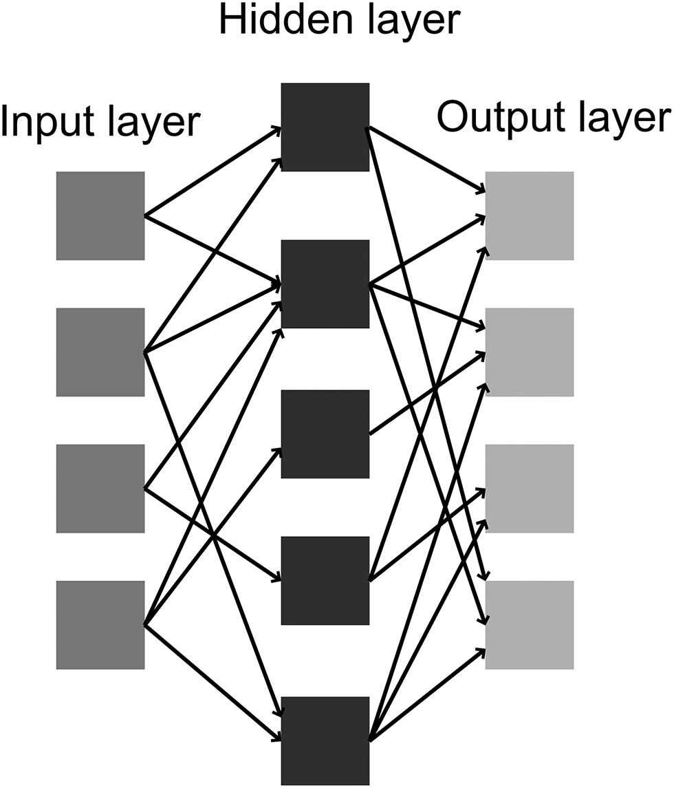
Example of neural network setup connections between neutron layers.
In the case the sigmoid neuron contains N inputs with corresponding weights wj and bias b applied the formulation of activation function reads:
The particular choice of activation function determines the neural response to the neural network and has impact on its learning properties and capabilities.
Fundamental feature of neural network is its ability to learn based on teaching data sets. The process aims to find optimal solution for the specified task. For this purpose a cost function is defined which is a measure of particular solution distance from the optimal one. It is the key task of learning algorithms to minimize the cost function in the solution space. The least squares method defined on the observed data and neural network output is a typical approach characterizing the cost function. There are three learning paradigms, namely supervised learning, unsupervised learning and reinforcement learning. In supervised learning the two sets of paired data are given over which the neural network is trained to find optimal synapses weights, that match the presented, teaching data. The unsupervised learning is the process where for particular teaching data set the specific cost function chosen is minimized. The cost function is of arbitrary choice that should reflect any of the data features. In reinforcement learning the teaching data set is not given, instead so-called software agent (that is a computer program communicating with the environment) acts on the studied environment at some time t and observes its reaction. The aim of this action is to determine a scheme that minimizes measure cost function in long term. The neural network models are able to approximate, predict, or recognize specific behavior; they are also capable of making generalizations exceeding boundaries of range for which they were trained.
Lobato et al. [37] present a study in which three different types of neural networks are tested to model a polybenzimidazole-based polymer electrolyte membrane fuel cell. Multilayer Perceptron (MLP), Generalized Feedforward Network (GFF), and Jordan Elman Network (JEN) were used having as common characteristic the supervised learning control. The training and validation data set consisted of 16 series of experimental data where 10 % of the whole set were preserved for validation phase, which was not used for training the neural network purposes. The neural networks had three input variables: conditioning temperature, the operating temperature and electric potential, and three outputs: the electric current density, the cathode resistance and the ohmic resistance. The best prediction was reached by MLP network as determined at the validation stage, which was the simplest network used in the study. All three neural networks exhibited good accordance with experimental results, although.
Modeling the performance of Nafion type fuel cell was also subject of the study by Lee et al. [38] The aim of this analysis was to obtain an empirical model including process variations to estimate the performance of fuel cells without complex calculations. Artificial neural network were trained to fit experimental data obtained in a single cell in H2/air operation using Nafion 115 and Nafion 1135 membrane electrolytes. The models presented accounted for the current density, the gas pressure, temperature, humidity, and utilization to cover operating processes. The multilayer feed forward neural network was used with two cases of activation function for neurons, linear and tangent sigmoid function:
Due to the multilayered network construction the output of the jth hidden layer unit is given by:
where w’ji is the weight of connection from ith input unit to jth hidden layer unit and b’j is the bias value for jth hidden layer unit. The output value from the network is given by:
where wj is the weight of synapse from jth hidden layer unit to output unit and b is the bias for output unit. Finally the weights are adjusted to minimize sum of squares error SSE:
In the above the variable u is the velocity vector, ρ is the fluid density, g is the acceleration vector. The first equation states that the rate of change of force vector exerted on fluid volume ρ·∂u/∂t equals: the negative value of advective (sometimes referred to as convective) component of flow due to the fluid’s bulk motion ρu·∇u; the negative value of pressure gradient ∇p acting on the analyzed fluid volume; and bodyforces ρg exerted on a fluid volume. The bodyforces source term can be of different nature, typically due to gravity but also centrifugal, magnetic or porous media resistance forces can be taken into account. The second equation presenting zeroth divergence of velocity vector means that there are no source or sinks in the volume analyzed. The key weakness of the equation is its idealization due to the absence of constitutive relation. For the fluids in motion it is very important to account for their real behavior by including the relation between forces applied (stress) and deformations observed (strain) on the fluid volume. This term was introduced by Navier and Stokes independently, extending the Euler’s equation and is referred to as stress-strain relation. For compressible fluids (most general case) the constitutive relation is presented in the form of total stress tensor σ (containing axiatoric and deviatoric components) that reads:
where λ is the bulk viscosity which originates from the drag forces created by volumetric change (compressibility effects). The identity matrix I was introduced during derivation due to fluid isotropic properties related to axiatoric component of the stress. The deviatoric component τ of the stress tensor σ originates from the viscous drag forces developing in fluid in motion:
The deviatoric stress tensor τdescribes the state of stress at a point inside a fluid in the deformed state. The deviatoric stress (apart from axiatoric which is an uniform stress) has dissipative nature and is referred to as diffusion of momentum term. The variable μ is the viscosity of the fluid.
Any source of vector or tensor quantity is indicated by the its divergence, therefore the divergence of the stress tensor describes the force transport component that results from the viscous nature of the fluid. The divergence of deviatoric stress tensor τ reads:
which finally leads to the formulation of Navier–Stokes equation:
The above equation is valid for constant viscosity Δ which does not depend on strain rate (Newtonian fluids). Another terms that appear in this equation: Δ∇2u is the momentum diffusion, the gradient of the divergence of velocity ∇(∇·u) – the resultant vector field presents the measure of the changes of the source/sink of the velocity vector field of the fluid volume. The Navier–Stokes equation itself describes the velocity field of the fluid modeled.
The mass continuity equation might also be considered. The solution of conservation of mass equation:
results in scalar field describing mass distribution in the fluid volume. The equation describes the fact that the rate of change of mass ∂ρ/∂t inside specified volume of fluid equals the difference between masses entering and exiting ∇·(ρu) this volume. For the multicomponent flows additional diffusive terms must be accounted for:
where ∇·(D∇ρ) is the measure of the changes of flux due to diffusion, D is the diffusion coefficient. In case of reactive flows the equation might preferably be expressed using molar basis and for nonequimolar chemical reaction additional source term S should be introduced.
3.1.1 Finite volume method
A practical realization of solution algorithms to the Navier–Stokes equations is a finite volume method widely known as CFD. The finite volume refers to the discretization approach used, which is most popular in fluid dynamics simulation software packages. The governing form of the finite volume equation reads:
which formulates the principia that changes in time are balanced by changes in space. The vector of conserved variables Q is integrated over a volume V, while fluxes vector F is integrated over boundary surface A surrounding fluid volume V.
The Navier–Stokes equation solution is obtained by applying appropriate discretization scheme over time, for time derivative of function u:
In this way the partial differential equation is discretized to give ordinary differential equations set. The spatial derivatives follow similar schema (although different schema are used), for the x component of u:
The above scheme represents a general guideline of discretization. In typical practice the geometry of analyzed object is constructed by spatial mesh which can be assembled of number of cells. Such volumetric cells can be chosen as tetrahedrons, wedges, prisms, hexahedrons and polyhedrons for three-dimensional cases. For modeling in two dimensions it is typical to use triangles, rectangles or quadrilateral to represent the space of the flow. It is important to mention that the geometric primitives used are of convex type.
The process of mesh creation is the preprocessing stage where a decision is made about the sizes and shapes of boundaries, eventually moving or rotating bodies, and the type and size of the mesh cells used. This is crucial to the accuracy of the solution for the cell size not to be larger than the smallest process phenomena to be tracked and simulated. From this point it is evident that to be able to solve or represent very small flow effects one should also use very small cell sizes, which in turn would increase the cells number. Because the differential equations are discretized over the cells producing corresponding number of algebraic equations, the higher number of cells results in larger equations set to be solved. Consequently as a reason of increasing demands on accuracy, decreasing size of cells produces CFD models that require more time to reach the solution. This is a problem of tradeoff between the demanded accuracy and computing load when performing the step of preprocessing. The preprocessed mesh is then a base of the core step – the processing that consists on applying the iterative algorithms to obtain the solution for steady or transient states of the flow. The final stage is to postprocess the results obtained to analyze them. It can be the graphical representation of the flows but also calculation of several process variables, e.g. calculating flowrates, pressure drops, or chemical reaction rates.
Reformulating the Navier–Stokes eq. (50) to account for transport through porous media an additional source force term S must be introduced:
which accounts for the resistance effects when modeling permeate flux. For any type of membrane, polymer, ceramic, and so forth when the sieve transport is considered the most straightforward way to calculate the S resistance term is to use Darcy equation.
and inertial losses factor:
In the above formulation the multiplication of both the vector R (inertial resistance factor which for non-isotropic media depends on direction) and vector u is a scalar product. The velocity vector magnitude is designated by |u|. The resistance term S in the Navier–Stokes equation is the summation of both component resistances. For the case when the membrane material can be assumed to be isotropic, then the geometric direction ith component of S reads:
The variable α is the permeability and R is the inertial resistance factor. For the isotropic case the indexes are omitted. The simple and straightforward estimation of both the parameters can be done on the basis of experimental measurements of the flows and pressures across the membrane [40]. Inertial resistance term R can be calculated based on measurements of the permeate flux q subject to changing transmembrane pressure Δ p:
Having calculated the R coefficient and knowing the membrane thickness L the permeability coefficient is obtained by relation:
Many software tools aimed for CFD calculations which allow fluid transport in porous media simulation, provide specific interface to enter these component resistances, in different range of functionality, however (e.g. Ansys/Fluent allows for vector resistance specifications while CFX allows only a scalar definition, concerning version 16.0).
Pellerin et al. [41] used Darcy law to simulate a two-dimensional case of membrane flux. The fluid flow outside membrane is simulated using closure model for turbulence effects (density-weighted ensemble-averaged, which is a simpler case of Reynolds averaged stress model). The membrane itself is simulated as an isolated entity by the laminar flow approach with velocity calculated on the basis of Darcy equation. The two-dimensional space was constructed by regular mesh of squares which formulated simple discretization problem of finite differences approach. The results were compared to analytical models of Berman [42] and Gupta [43]. The model proposed and both literature models show similar results which support it accuracy.
The CFD simulation of porous membrane of fuel cell is presented by Wang et al. [44] For the first time, the polarization curve and flowing components concentration distributions encompassing both single- and two-phase regimes of the air cathode are presented. The liquid and vapor transfer is governed by capillary transport mechanism and molecular diffusion, respectively, due to negligible small air velocity within the porous electrode. Authors applied following simplifying assumptions to the CFD model presented: the gas diffusion is isotropic and homogeneous, and characterized by an effective porosity and permeability of the porous media; the catalyst layer is treated as an infinitely thin surface for oxygen reduction at the membrane interface forming water; the cell is at isothermal conditions; the gas phase is an ideal mixture. The model construction allows for algorithmic coupling to predict the transition between the single and two phase regimes of flow. The two-phase model is appropriate to model the air cathode of both hydrogen and direct-methanol fuel cells.
The three-dimensional model of polymer membrane fuel cell was presented by Siversten et al. [45] The model proposed was non-isothermal model for proton exchange membrane fuel cells, which was implemented into a CFD code. The model algorithm presented allows for parallelization of the computing architecture. The convective and diffusive transport mechanism was accounted for which allows to present the concentration distribution of components. Appropriate energy balance is used to render the distributed heat generation associated with the electrochemical reaction in the cathode and anode. Authors implemented the modeling procedure in commercial tool Fluent 6.1 by the use of so-called user-defined functions, which allows to program own algorithms using C programming language. The modeling algorithm included flow channels and membrane itself. For the membrane the electro-neutrality was assumed, which is a valid assumption for fully humidified polymer material. The heat transport through the membrane for N-component mixture is calculated by the energy balance equation that reads:
where E is the total energy, keff is the effective conductivity, Jj is the diffusive flux and H is the enthalpy of the jth specie. The effective stress tensor matrix is designated by τeff (is the volume average of the stress matrix [46] as given by (48)) and Sh is the source term for energy per unit volume and unit time which may include the heat of reaction. A general thermodynamic approach is used to model the transport in the membrane material. The current density of protons j is given by:
where L++ is the specific proton conductivity [47] (assumed at value 13.375 S/m), ϕm is the local potential, Δ w is the local chemical potential of water. The water flux is given by:
The L variables are the Onsager coefficients, and can be related by L+w=Lw+. They can be estimated by the equation:
where ξ is the number of water molecules transported with each proton (value of 3 is used). The variable F is the Faraday constant. The variable Lww is not discussed in the paper unfortunately, the reader is referred to master thesis of Sivertsen [48]. The lmem variable is used (permeability of the membrane, 2.35·10–7 mol2s/m–3kg–1):
The number of cells of a mesh constituting the space of simulation was total of 546,000. Such a mesh resolution is typically sufficient to obtain accurate and reliable results. Global comparisons show that the model and experimental results are in good accordance. The study also demonstrates that altering the conductivity modifies the current distribution by changing the relative influence of electrode potential to activation overpotentials (measure of electrode polarization).
Wiley et al. [49] present a two-dimensional study to compare the CFD simulations results with previous literature experimental data. The developed approach was a general purpose model of concentration polarization and fluid flow in pressure driven membrane separation processes. The model treats the channels as a typical space of flow with no slip boundary conditions at the walls. The membrane wall is treated differently although, where the tangential velocity component is applied to be zero and normal component of velocity (entering the space of membrane material) uw is defined by:
where u0 is the velocity at channel inlet, cw is the concentration at the wall, c0 is the channel inlet concentration. The coefficient β is given by Brian [50] as:
and R (fractional component rejection/retention):
where J is the component flux through membrane. The variable π0 is the osmotic pressure of the feed solution, and Δ P is transmembrane pressure.
The normal velocity uw to the membrane surface can also be given by relation of Doshi et al. [51]:
although no further details are given referring constants B1 and B2. The variable h represents the half flow channel height, and Sc is the Schmidt number. The main concept is to balance the convective flux in the channel with the diffusive flux in the membrane material, taking into account that not all of the fluid pass through the membrane. This last is taken into account by R rejection coefficient. Finally the balance equation at the feed side of the membrane reads:
and for the permeate side:
where D is the diffusion coefficient in the membrane (the term D∂c/∂y formulates the diffusive flux along y axis). The CFD model developed contains specific equations for the cases studied, but it can be changed to cover any combination of variations in wall flux, rejection, viscosity and diffusivity.
3.2 Boltzmann lattice models
The Boltzmann lattice method is completely different method of solving Navier–Stokes equations than the finite volume approach. The method is based on the Boltzmann equation which describes the statistical behavior of a non-equilibrium thermodynamic system. The equation in the principal formulation can be stated as:
In the above formulation f is the distribution function which quantifies particles per unit volume in single-particle phase space. It is a function of six scalar coordinates of phase space of position and momentum components: (r, p) = (x, y, z, px, py, pz) which is parametrized by time t. The force term relates to the forces of external origins exerted on the particles, the diffusion term characterizes the diffusion of particles, and collisions is the collision term – describing for the forces appearing between particles in collisions. The specific formulation of this equation reads:
where m is the mass of the particles ensemble with which the function f is associated. Vector F is the external forces vector (e.g. force due to gravity), vector p is the momentum vector, vector r is the position of the particle. The term for collisions cannot be formulated generally. The simplest model of collisions between particles is due to Bhatnagar, Gross and Krook [52] which assumes that the effect of molecular collisions is to shift the distribution function f being in non-equilibrium state back to a Maxwellian equilibrium distribution function f0, with the rate proportional to the molecular collision frequency υ:
Considering the mixture of the N components the general formulation for kth specie reads:
where apostrophe superscripted variables refer to the state after collision. The variable Ω is the solid scattering angle, the term σ(Ω) is the differential cross section for collision with the scattering angle Ω.
The Lattice Boltzmann model refers to a small differential volume in six-dimensional space of position and momentum. The idea goes further in problem reduction with the postulate that the particle (or fluid ensemble) is restricted to move in specific directions only or stay at rest. For the case of two physical dimensions of fluid calculations, these directions
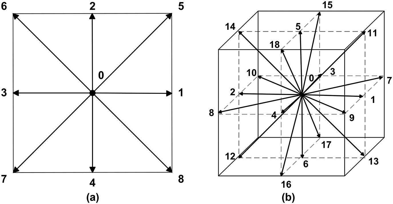
Lattice Boltzmann microscopic speed directions setup for two (D2Q9) and three (D3Q19) dimensional physical space.
The designations refer to the physical dimensions D and number of directions chosen Q over which the movement is quantified. For presented case of D2Q9 lattice the microscopic velocities are defined by:
where c is the lattice speed:
The value of ∇ x is the lattice cell geometric size (geometric discretization size), the ∇ t is the time step of transient discretization. The resultant value of velocity for given lattice cell with Ndir directions is then the macroscopic velocity u(x, t) which is given as the average weighted by distribution function fi:
while density ρ is given by the summation of the distribution function:
The Lattice Boltzmann method can be regarded as a particular finite difference method for solving the Boltzmann transport equation on a lattice. The key explanation why this approach can function as a method for fluid simulations is that the Navier–Stokes equations can be derived from the discrete equations by the Chapman–Enskog expansion [53].
Park et al. [54] apply the lattice Boltzmann method to the multi-phase flow phenomenon in the inhomogeneous gas diffusion layer of a polymer electrolyte membrane fuel cell. The D2Q9 lattice was used to represent the two-dimensional process of flow and D3Q15 for three physical dimensions. The Stokes/Brinkman [55] model formulation was used to describe the flow in porous media:
The operator
The permeability tensor elements on the diagonal (kxx, kyy, kzz) represent the components of permeability corresponding to pressure force acting in the direction of flow. The off-diagonal permeability tensor elements (kxy, kxz, kyx, kyz, kzx, kzy) account for the flow rate dependence on pressure forces in orthogonal directions. Equation 73 is coupled with the continuity equation:
The construction of lattice Boltzmann model is done by formulating the collision term according to BGK method [52], with time discrete advancement function defined as:
where ∇ t is the numerical time step, τυ is the relaxation time. The equilibrium distribution function
The microscopic velocities are formulated by Cartesian coordinates given by definition:
which resembles the definition given by formulation (77).
The three-dimensional construction of the lattice is formed used 15 microscopic speeds defined by the matrix:
The equilibrium distribution function
for zeroth microscopic speed:
for orthogonal directions of microscopic speeds, i=1..6:
for non-orthogonal microscopic speeds, i=7..14:
For the porous media lattice Boltzmann model is modified to account for Brinkman equation by incorporating the force term FB that reads:
and:
The term U exchanges the velocity u in formulation for equilibrium distribution function fieq. The variable s(x,t) indicates the porous media (=1) or void (=0) of the space of the flow.
The force term F(x,t) which is needed to recover the Brinkman equation reads:
where the β parameter describes the momentum sink magnitude due to resistance of porous media. Finally the lattice Boltzmann equation according to Brinkman porous material description reads:
in which the β parameter:
In the above the viscosity υ and permeability tensor are expressed in lattice units [56].
Han et al. [57] presents the results of the two-dimensional simulation concerning the polymer membrane of fuel cell although no specific details concerning mathematical procedure taken are given in the study. The transport is considered in two regimes: flow in microporous layer and in gas diffusion layer. The numerical investigations concentrate primarily on liquid water transport in flooding conditions. The water entering the porous regions is generally driven by the capillary forces through the contact with the solid material. Numerical results acquired for the cases with and without the perforated cavity in the porous layers were compared. For the case without the perforated cavity, water randomly penetrates through the porous regions and finally appears as two small droplets at the surface of the channel. For the case with the hole in the porous layer, water transports favorably through this void space and appears as a relatively large liquid droplet at the open end. This liquid transport phenomenon is caused by the smaller capillary pressure requirement and less flow resistance in the large perforated pore. The perforated pores can therefore function as a suitable water transport pathway and contribute in liquid water removal.
Kim et al. [58] investigated liquid water transport in the microporous layer and gas diffusion layer of polymer electrolyte membrane fuel cells by lattice Boltzmann method. Application of the model for two-phase systems with porous geometry that emulates the process in multilayer porous transport layers. The model was built for two-dimensional physical space. Apart from the typical lattice Boltzmann setup (D2Q9) the approach to calculate collision function is aimed at the liquid–liquid and liquid–solid interactions. The collision function for the jth component and ith microscopic speed applied reads:
where τj is relaxation time corresponding to viscosity of specie jth given by:
The variable cs is the speed of sound in the media simulated. The equilibrium distribution function is then given by:
The equilibrium velocity of the specie jth is formulated by considering the rate of momentum change due to the fluid–fluid and fluid–solid interaction forces ΣFj . In the study the ΣFj does not account for gravitational and buoyancy forces, and is given by:
The rate of net momentum change due to the fluid–fluid interactions Fjint are given by:
where ψj is the effective number density for specie jth and is equal to its density ρj for multiphase lattice Boltzmann model. The function Gj,k(x, x’) is the Green function [59] which relates the interactions between specie jth at x location and x’ location, that reads:
which means that only the nearest particle interactions are considered, the coefficient Gj,k is defined to account for the strength of the interaction between components j and k. The Gj,k determines the repulsion strength between particles belonging to different species and can be used to fine tune the surface tension between phases. For critical value of Gj,k the repulsion forces are not strong enough to keep the two fluids separated and start to form single phase system [60]. The fluid–solid interactions are considered by the relation:
where Gjads is the adsorption coefficient for specie jth. The Gjads controls the strength of the fluid wettability of the solid surface. The function s(x+ei∇ t) attains value 1 for solid neighbor location and 0 for fluid neighborhood.
The model studied presents creation of water clusters inside the porous media. Also extraordinary transient behavior of the liquid water near the microporous layer/gas diffusion layer interface and the gas diffusion layer/gas channel interface was realized from the lattice Boltzmann simulations of highly hydrophobic multilayer porous transport layers.
3.2.1 Summary
CFD methods are valuable tools for process engineers in the design and simulation fields. The differential models, commonly referred to as CFD, aim to solve the Navier–Stokes equation in its discretized form. The advantage of this approach is the ability to use a variety of discretization schemes that suits the geometrical and process needs. The discretization which is dependent on the mesh construction is always a source of error which can be minimized by proper tuning the cell sizes, shapes and types. This formulation of the fluid dynamics approach is not able to predict the thermodynamics of the simulated entity, however. On the other hand, the lattice Boltzmann method, by proper use of collision operator, is able to predict specific thermodynamic behavior of the fluids simulated, e.g. the existence of multiphase system. Such possibility, in order to be incorporated into traditional discrete approach, needs to be accounted for by separate models, for example volume of fluid model of multiphase flow, which further enlarges the formulation and computing demand. One of the key benefits of lattice Boltzmann method for simulating fluid flows as compared to traditional numerical methods is their aptitude to efficiently model interfaces between two or more fluids. Both the fluid dynamics approaches, however totally different, can successfully be incorporated into modeling and simulations of membrane systems.
Acknowledgment
This article is also available in: Tylkowski, Polymer Engineering. De Gruyter (2017), isbn 978-3-11-046828-1.
References
1. Sampson RA. On Stokes’s current function. Phil Trans R Soc Lond A. 1891;182:449–518.10.1098/rsta.1891.0012Search in Google Scholar
2. Song L, Elimelech M. Theory of concentration polarization in crossflow filtration. J Chem Soc Faraday Trans. 1995;91(19):3389–3398.10.1039/ft9959103389Search in Google Scholar
3. Happel J, Brenner H. Low Reynolds number hydrodynamics. Englewood Cliffs: Prentice Hall, 1965.Search in Google Scholar
4. McCabe WL, Smith J, Harriott P. Unit operations of chemical engineering.. New York: McGraw-Hill Education, 2005Search in Google Scholar
5. Aimar P, Baklouti S, Sanchez V. Membrane – solute interactions: Influence on pure solvent transfer during ultrafiltration. J Memb Sci. 1986;29(2):207–224.10.1016/S0376-7388(00)82470-9Search in Google Scholar
6. Velicangil O, Howell IA, Le MEH, Zeppelin AL. Ultrafiltration of protein solutions. Annals NY Acad Sci. 1981;369:35510.1111/j.1749-6632.1981.tb14202.xSearch in Google Scholar
7. Chung T-S, Jiang LY, Li Y, Kulprathipanja S. Mixed matrix membranes (MMMs) comprising organic polymers with dispersed inorganic fillers for gas separation. Prog Polym Sci. 2007;32(4):483–507 2007.10.1016/j.progpolymsci.2007.01.008Search in Google Scholar
8. Maxwell JC. Treatise on electricity and magnetism. London: Oxford University Press, 1873.Search in Google Scholar
9. Mahajan R, Burns R, Schaeffer M, Koros WJ. Challenges in forming successful mixed matrix membranes with rigid polymeric materials. J Appl Poly Sci. 2002;86:881–890.10.1002/app.10998Search in Google Scholar
10. Slesarenko VV. Modelling of RO installations for wastewater treatment plants. Pac Sci Rev. 2014;16(1):40–44 2014. ISSN 1229-5450.10.1016/j.pscr.2014.08.008Search in Google Scholar
11. Fraga SC, Trabucho L, Brazinha C, Crespo JG. Characterisation and modelling of transient transport through dense membranes using on-line mass spectrometry. J Memb Sci. 2015;479:213–222 2015.10.1016/j.memsci.2014.12.016Search in Google Scholar
12. Kreulen H, Smolders CA, Versteeg GF, Van Swaaij WPM. Microporous hollow fibre membrane modules as gas-liquid contactors Part 2. Mass transfer with chemical reaction. J Memb Sci. 1993;78(3):217–238.10.1016/0376-7388(93)80002-FSearch in Google Scholar
13. Dindore VY, Brilman DWF, Versteeg GF. Hollow fiber membrane contactor as a gas–liquid model contactor. Chem Eng Sci.60(2):467–479 2005.10.1016/j.ces.2004.07.129Search in Google Scholar
14. Sundaramoorthy S, Srinivasan G, Murthy DVR. An analytical model for spiral wound reverse osmosis membrane modules: Part II – Experimental validation. Desalination.277(1–3):257–264 2011.10.1016/j.desal.2011.04.037Search in Google Scholar
15. Criscuoli A, Carnevale MC, Drioli E. Modeling the performance of flat and capillary membrane modules in vacuum membrane distillation. J Memb Sci. 2013;447:369–375 2013.10.1016/j.memsci.2013.07.044Search in Google Scholar
16. Warshel A, Levitt M. Theoretical studies of enzymic reactions: Dielectric, electrostatic and steric stabilization of the carbonium ion in the reaction of lysozyme. J Mol Biol. 1976;103(2):227–249.10.1016/0022-2836(76)90311-9Search in Google Scholar
17. Slater JC. Atomic shielding constants. Phys Rev. 1930;36:57.10.1103/PhysRev.36.57Search in Google Scholar
18. Ditchfield R, Hehre WJ, Pople JA. Self‐consistent molecular‐orbital methods IX. An extended Gaussian‐type basis for molecular‐orbital studies of organic molecules. J Chem Phys. 1971;54(2):724–728.10.1063/1.1674902Search in Google Scholar
19. Levine IN. Quantum chemistry.. Englewood Cliffs, NJ: Prentice Hall, 1991.Search in Google Scholar
20. Hehre WJ. A guide to molecular mechanics and quantum chemical calculations. Irvine, CA: Wavefunction, Inc, 2003.Search in Google Scholar
21. Cramer CJ. Essentials of computational chemistry.. Chichester: John Wiley & Sons, Ltd, 2002.Search in Google Scholar
22. Jensen F. Introduction to computational chemistry.. New York: John Wiley and Sons, 1999Search in Google Scholar
23. Quinn CM. Computational quantum chemistry: An interactive introduction to basis set theory, 1st ed London: Academic Press, 2002Search in Google Scholar
24. Yu TH, Sha Y, Wei-Guang Liu BV, Merinov PS, Goddard WA. Mechanism for degradation of Nafion in PEM fuel cells from quantum mechanics calculations. J Am Chem Soc. 2011;133(49):19857–19863.10.1021/ja2074642Search in Google Scholar PubMed
25. Yu TH, Liu W-G, Sha Y, Merinov BV, Shirvanian P, Goddard III WA. The effect of different environments on Nafion degradation: Quantum mechanics study. J Memb Sci. 2013;437:276–228 2013.10.1016/j.memsci.2013.02.060Search in Google Scholar
26. Sakai H, Tokumasu T. Quantum chemical analysis of the deprotonation of sulfonic acid in a hydrocarbon membrane model at low hydration levels. Solid State Ionics. 2015;274:94–99.10.1016/j.ssi.2015.03.005Search in Google Scholar
27. Paddison SJ, Elliott JA. Molecular modeling of the short-side-chain perfluorosulfonic acid membrane. J Phys Chem A. 2005;109(33):7583–7593.10.1021/jp0524734Search in Google Scholar PubMed
28. Shah MR, Yadav GD. Prediction of sorption in polymers using quantum chemical calculations: Application to polymer membranes. J Memb Sci. 2013;427:108–117 2013.10.1016/j.memsci.2012.09.037Search in Google Scholar
29. Vosko SH, Wilk L, Nusair M. Accurate spin-dependent electron liquid correlation energies for local spin density calculations: A critical analysis. Can J Phys. 1980;58(8):1200.10.1139/p80-159Search in Google Scholar
30. Gear GW. Numerical initial value problems in ordinary differential equations. Englewood Cliffs, NJ: Prentice‐Hall, 1971.Search in Google Scholar
31. Verlet L. Computer “experiments” on classical fluids. I. Thermodynamical properties of Lennard−Jones molecules. Phys Rev. 1967;159:98–103.10.1103/PhysRev.159.98Search in Google Scholar
32. Shen M, Keten S, Lueptow RM. Rejection mechanisms for contaminants in polyamide reverse osmosis membranes. J Memb Sci. 2016;509:36–47.10.1016/j.memsci.2016.02.043Search in Google Scholar
33. Edward Harder D, Walters E, Bodnar YD, Faibish RS, Roux B. Molecular dynamics study of a polymeric reverse osmosis membrane. J Phys Chem B. 2009;113(30):10177–10182.10.1021/jp902715fSearch in Google Scholar PubMed
34. Devanathan R, Idupulapati N, Baer MD, Mundy CJ, Dupuis M. Ab initio molecular dynamics simulation of proton hopping in a model polymer membrane. J Phys Chem B. 2013;117(51):16522–16529.10.1021/jp410229uSearch in Google Scholar PubMed
35. Ling C, Liang X, Fan F, Yang Z. Diffusion behavior of the model diesel components in different polymer membranes by molecular dynamic simulation. Chem Eng Sci. 2012;84:292–302 2012.10.1016/j.ces.2012.08.035Search in Google Scholar
36. Bader R. Atoms in molecules: A quantum theory. New York: Oxford University Press, 1994.Search in Google Scholar
37. Lobato J, Cañizares P, Rodrigo MA, Linares JJ, Piuleac C-G, Curteanu S. The neural networks based modeling of a polybenzimidazole-based polymer electrolyte membrane fuel cell: Effect of temperature. J Power Sources. 2009;192(1):190–194 2009.10.1016/j.jpowsour.2009.01.079Search in Google Scholar
38. Lee W-Y, Park G-G, Yang T-H, Yoon Y-G, Kim C-S. Empirical modeling of polymer electrolyte membrane fuel cell performance using artificial neural networks. Int J Hydrogen Energy.29(9):961–966 2004.10.1016/j.ijhydene.2003.01.002Search in Google Scholar
39. Chakraborty S, Dasgupta J, Farooq U, Sikder J, Drioli E, Curcio S. Experimental analysis, modeling and optimization of chromium (VI) removal from aqueous solutions by polymer-enhanced ultrafiltration. J Memb Sci. 2014;456:139–154 2014.10.1016/j.memsci.2014.01.016Search in Google Scholar
40. Staszak M, Staszak K. Computational fluid dynamics (CFD) modelling of porous, ultrafiltration membranes. J Membr Separation Technol. 2013;2(1):36–46.10.6000/1929-6037.2013.02.01.4Search in Google Scholar
41. Pellerin E, Michelitsch E, Darcovich K, Lin S, Tam CM. Turbulent transport in membrane modules by CFD simulation in two dimensions. J Memb Sci. 1995;100(2):139–153 1995.10.1016/0376-7388(94)00250-3Search in Google Scholar
42. Berman AS. Laminar flow in channels with porous walls. J Appl Phys. 1953;24:1232–1235.10.1063/1.1721476Search in Google Scholar
43. Gupta BK, Levy EK. Symmetrical laminar channel flow with wall suction. Trans ASME J Fluids Eng. 1976;98:469–474.10.1115/1.3448373Search in Google Scholar
44. Wang ZH, Wang CY, Chen KS. Two-phase flow and transport in the air cathode of proton exchange membrane fuel cells. J Power Sources. 2001;94(1):40–50 2001.10.1115/IMECE2000-1363Search in Google Scholar
45. Sivertsen BR, Djilali N. CFD-based modelling of proton exchange membrane fuel cells. J Power Sources. 2005;141(1):65–78 2005.10.1016/j.jpowsour.2004.08.054Search in Google Scholar
46. Dhont JKG. An introduction to dynamics of colloids.. Amsterdam: Elsevier, 1996Search in Google Scholar
47. Janssen GJM. A phenomenological model of water transport in a proton exchange membrane fuel cell. J Electrochem Soc. 2001;148(12) A1313–A1323.10.1149/1.1415031Search in Google Scholar
48. Sivertsen BR. CFD-based modelling of proton exchange membrane fuel cellsNorwegian University of Science and Technology, 2003, Master’s thesis.Search in Google Scholar
49. Wiley DE, Fletcher DF. Techniques for computational fluid dynamics modelling of flow in membrane channels. J Memb Sci. 2003;211(1):127–137 2003.10.1016/S0376-7388(02)00412-XSearch in Google Scholar
50. Brian PLT. Concentration polarization in reverse osmosis desalination with variable flux and incomplete salt rejection. Ind Eng Chem Fundam. 1965;4(4):439–445.10.1021/i160016a014Search in Google Scholar
51. Doshi MR. The effect of concentration dependent viscosity and diffusivity on concentration polarization in reverse osmosis flow systems. AIChE Symp Ser. 1971;68:124.Search in Google Scholar
52. Bhatnagar PL, Gross EP, Krook M. A model for collision processes in gases. I. Small amplitude processes in charged and neutral one-component systems. Phys Rev. 1954;94(3):511–525.10.1103/PhysRev.94.511Search in Google Scholar
53. Bardos C, Ukai S. The classical incompressible Navier-Stokes limit of the Boltzmann equation. Math Models Methods Appl Sci. 1991;01(02):235–257.10.1142/S0218202591000137Search in Google Scholar
54. Park J, Li X. Multi-phase micro-scale flow simulation in the electrodes of a PEM fuel cell by lattice Boltzmann method. J Power Sources. 2008;178(1):248–257 2008.10.1016/j.jpowsour.2007.12.008Search in Google Scholar
55. Park J, Matsubara M, Li X. Application of lattice Boltzmann method to a micro-scale flow simulation in the porous electrode of a PEM fuel cell. J Power Sources. 2007;173(1):404–441 2007.10.1016/j.jpowsour.2007.04.021Search in Google Scholar
56. Latt J. Hydrodynamic limit of lattice Boltzmann equationsUniv. Genève, 2007 – Sc. 3846-2007/03/09, PhD thesis.Search in Google Scholar
57. Han B, Meng H. Numerical studies of interfacial phenomena in liquid water transport in polymer electrolyte membrane fuel cells using the lattice Boltzmann method. Int J Hydrogen Energy. 2013;38(12):5053–5059 2013.10.1016/j.ijhydene.2013.02.055Search in Google Scholar
58. Kim KN, Kang JH, Lee SG, Nam JH, Kim C-J. Lattice Boltzmann simulation of liquid water transport in microporous and gas diffusion layers of polymer electrolyte membrane fuel cells. J Power Sources.278:703–717 2015.10.1016/j.jpowsour.2014.12.044Search in Google Scholar
59. Shan X, Doolen G. Multicomponent lattice-Boltzmann model with interparticle interaction. J Stat Phys. 1995;81(1):379–393.10.1007/BF02179985Search in Google Scholar
60. Parmigiani A.. Lattice Boltzmann calculations of reactive multiphase flows in porous mediaUniversite de Geneve, , 2010. PhD thesis.Search in Google Scholar
© 2017 Walter de Gruyter GmbH, Berlin/Boston
Articles in the same Issue
- Computational methods in preformulation study for pharmaceutical solid dosage forms of therapeutic proteins
- Polymer application for separation/filtration of biological active compounds
- DFT study of anthocyanidin and anthocyanin pigments for Dye-Sensitized Solar Cells: Electron injecting from the excited states and adsorption onto TiO2 (anatase) surface
- Green chemistry education in the Middle East
- Polymer additives
- Nanodiamonds for Biological Applications
- Modeling and simulation of membrane process