Veto Bargaining with Incomplete Information and Risk Preference: An Analysis of Brinkmanship

3.1 Payoffs

Players’ payoffs are constructed from period utilities. When the offer is rejected, both players receive 0 utility for the period. This is the disaster that can happen for the players.^[6] When the offer is accepted, the proposer’s utility for the period is

where u is the following constant absolute risk aversion (CARA) utility function.

I use CARA utility for the proposer to model the proposer’s risk aversion. CARA utility has useful proprieties that help me to analyze the relation between the proposer’s risk aversion and the proposer’s equilibrium strategies. The most important one is that by Pratt (1964)’s theorem 1, for CARA utility, the higher the proposer’s absolute risk aversion, η, the higher the risk premium. In other words, a more risk-averse proposer requires a greater payment in order for him to take the same amount of risk. Another useful property is that for any η, u(0) = 0. This helps me simplify many formulas.

When the offer is accepted, the vetoer’s utility for the period is

This means that I can interpret the vetoer as a risk-neutral vetoer with CARA utility. (Since the vetoer cannot engage in brinkmanship, her risk preference is not important for the results.) The greater a _t is, the more favorable the deal is to the vetoer and the less favorable the deal is to the proposer. This means that a _t can also be thought of as a payment offer from the proposer to the vetoer.

The proposer’s and the vetoer’s discount factors are respectively δ _P  ∈ (0, 1) and δ _V  ∈ (0, 1). Having separate discount factors lets me distinguish each player’s condition for the PBEs. Players’ maximize the expectation of the discounted sum of their utilities.

3.2 Players’ Types, S _P and S _V

The image of S _P is {p _L , p _H }. The image of S _V is {v _L , v _M , v _H }.^[7]

From the values, p _H is the greatest and p _L is between v _L and v _M .^[8] I denote the probabilities of p _L , p _H , v _L , v _M and v _H the following way.

When S _V  = v _L , S _V  = v _M or S _V  = v _H , I respectively say that the vetoer is low, medium or high type. I use these terms the same way for the proposer.

4.1 Risk-Taking Equilibria

I define a risk-taking equilibrium (RTE) using players’ strategies.

Note that in the above definition, the proposer offers a ̲ regardless of his type when he believes b₀ and only offers v _H when he is high type and believes b_−L. In other words, when the proposer has gained no information about the vetoer’s type, the offer is a ̲ . When the proposer is high type and he believes that the vetoer is not low type, the offer is v _H . In other cases, he offers v _L .

From the vetoer’s strategy, (iv), (v) and (viii) are the important parts. By (iv) and (viii), when the vetoer’s type has not been revealed, the low type vetoer accepts a ̲ or greater and the medium and high type vetoer accepts v _H or greater. By (v), once the vetoer is revealed to be low type, vetoer accepts v _L . On the other hand, in (viii), once the vetoer is partially revealed to be not low type, vetoer accepts v _H .

Given the above strategies, I explain how the game plays on the equilibrium path for an RTE that is depicted in Figure 2. In the figure, the ovals contain the offers for the periods. In period 1, proposer always acts first believing b₀. So the first offer is a ̲ . All RTEs satisfy a ̲ < v H .^[11] By the vetoer’s strategy in (iv) and (viii), the low type vetoer accepts this and the medium or high type vetoer rejects this. So the disaster only occurs when the vetoer is low type. Given the different actions of different vetoer types, at the start of period 2, the proposer’s belief diverges. If the vetoer accepted, the proposer believes b _L , that the vetoer is low type. Otherwise, the proposer believes b_−L, that the vetoer is medium or high type. In other words, the vetoer’s decision in period 1 informs the proposer whether the vetoer is low type or not. On the equilibrium path, the following happens from period 2 and onwards. The high type proposer who believes b_−L always offers v _H which is always accepted but for all other cases, the offer is v _L . Also, the medium and high type vetoers reject v _L but on the equilibrium path, any other offer is accepted.

Figure 2:

Offers on the equilibrium path in an RTE.

The reason that the proposer initially offers a ̲ , an offer lower than v _H is to extract type information from the vetoer. If the proposer is high type, once he figures out that the vetoer is medium or high type, from period 2, he will offer v _H , the lowest offer that will be accepted by these types of vetoers. Once he figures out that the vetoer is low type, from period 2, he will offer v _L . In other words, the high type proposer is intentionally making an offer that the medium or high type will not accept to separate the low type vetoer. Once the low type vetoer is identified, both the low and high type vetoers use this information to offer only v _L from then. Both the low and high type proposers make the low offer ( a ̲ in this case) in defiance of the risk of rejection. Such strategies by any type are the “brinkmanship” of this paper and its key phenomenon.

The proposer’s strategy demonstrates the ratchet effect. Once a vetoer accepts an offer, the proposer does not offer a higher offer because the proposer knows that the vetoer is of a type that will accept the previous offer. In fact, when the initial low offer of a ̲ is accepted, the next offer v _L is even lower. This makes the vetoer reluctant to accept low offer not just because of the effect on current utility but because of the effect on future utilities as well. Therefore, the medium and high type vetoers reject the initial offer of a ̲ and build a reputation to be not the low type. Also, a ̲ must be sufficiently high that the low type vetoer considers it an adequate compensation for giving up the possibility of higher offers in the future.

In the RTEs, players sources of surplus are different. The proposer’s surplus comes from first-mover advantage and information about the vetoer. The first-mover advantage allows the proposer to propose a low policy or action that the vetoer would not propose. The proposer’s information about the vetoer lets him offer a low policy and action that will still be accepted.

On the other hand, the vetoer’s surplus comes from information rent. The vetoer’s information rent comes from the fact that the vetoer knows her own type but there are circumstances where the proposer thinks that the vetoer’s type can be higher. In period 1, the low type vetoer derives surplus from the fact that the proposer is unable to distinguish her from a medium or high type vetoer. In period 2, the medium type vetoer derives surplus from the fact that the proposer is unable to distinguish her from a high type vetoer. Vetoer’s expected payoff in an RTE is

The above proposition explains restrictions that let an RTE exist. (i) and (ii) are satisfied in any RTE. In (i), the left side is the expected cost of brinkmanship for the high type proposer. If brinkmanship fails, it is costly. The right side of (i) is the expected benefit of brinkmanship for the high type proposer. Brinkmanship is beneficial when it succeeds. In (ii), the right side is the expected payoff of the low type proposer when the vetoer is low type. (i) and (ii) contain δ P 1 − δ P on their right sides. δ _P is the discount factor for the proposer. In a RTE, a patient proposer of either type benefits more from the fact that from period 2, he can get a deal of v _L from the low type vetoer. Thus a more patient proposer has greater incentive for brinkmanship. (iii) guarantees that the medium type vetoer’s cut-off point in period 1 is v _H .

To explain (iv), I present Lemma 1. The proof of Lemma 1 and Proposition 1 in Appendix 1 and Lemma 3 in The Supplementary Material explain in more detail the progress and the beliefs of the game.

(iv) and Lemma 1 mean that in a RTE, the brinkmanship offer, a ̲ , is higher than v _L and the offer provides meaningful compensation to the low type vetoer. If the proposer is high type, rejecting a ̲ to have the proposer believe that the vetoer is not low type gives the low type vetoer positive expected utilities in the future. Therefore, the brinkmanship offer must compensate for not rejecting. (iv) and Lemma 1 also mean that a RTE needs to satisfy a ̲ < v H . If a ̲ ≥ v H , since all types of vetoers accepts a ̲ , the vetoer does not reveal any information about its type by accepting a ̲ . Since the proposer did not gain any information, the vetoer can get a ̲ offered again in the next period. This is not optimal for the low type proposer. A low f _H means that the proposer has a low probability of being the high type. A high δ _V means that the vetoer cares a lot about the future utility gain from rejecting the brinkmanship offer, a ̲ . (iv) and Lemma 1 shows that a low f _H and low δ _V make brinkmanship feasible.

The above proposition establishes the relationship between the proposer’s risk preference and the existence of RTEs. When the other parameters of the model and a ̲ allow for an existence of an RTE, an RTE exists when the proposer is sufficiently risk-seeking. η ̲ is the highest amount of risk aversion that allows an RTE to exist. Engaging in brinkmanship entails the risk of brinkmanship failure for the proposer. As a proposer becomes infinitely risk-seeking, he will come to value the potential gain from successful brinkmanship succeeds to be more valuable than the potential loss from failed brinkmanship. As a proposer becomes infinitely risk-adverse, he will come to feel the opposite way. Also, an infinitely risk-seeking proposer is willing to take a loss in period 1, for future gains.^[12] Therefore, under the proposition’s conditions, η ̲ always exists and is somewhere in the middle of those extremes. For any lower η, risk aversion, an RTE exists.

4.2 Risk-Avoiding Equilibria

The following defines the Risk-Avoiding Equilibrium (RAE).

The above definition defines the players’ strategies using the three beliefs defined in Definition 1, b _L , b_−L and b₀. For these beliefs, the proposer only offers v _H when he is high type and he believes b_−L or b₀ and in all other cases, he offers v _L . In other words, when the proposer thinks that the vetoer has a positive probability of not being the low type and gets positive utility from v _H being accepted, he offers v _H . When this is not true, the offer is v _L .

From the vetoer’s strategy, (iii) and (vi) are the important parts. In (iii), when the proposer thinks that the vetoer may be the low type, the low type vetoer’s cut-off point is v _L . In (vi), when the proposer believes that the vetoer may be the medium or high type, the medium or high type vetoer’s cut-off point is v _H .

Now that I have spelt out the players’ strategies, I will explain the progress of the game on the equilibrium path for an RAE. In all periods, the low type proposer offers v _L and the high type proposer offers v _H . The v _L offer is accepted by the low type vetoer and rejected by the medium and high type vetoers. The v _H offer is accepted by all types of vetoers.

This means that if the vetoer is low type, the high type proposer can make low offers (v _L in this case) and get it accepted in all periods. However, offering v _L entails the risk of rejection by the medium and high type vetoers. Thus, for the RAE, brinkmanship refers to the following strategy by the high type proposer. In period 1, he offers v _L . If it is accepted, he makes the same offer in subsequent periods. If it is rejected, he offers v _H in subsequent periods. This brinkmanship does not happen in the RAE because the proposer weakly prefers to not take the risk of rejection from the brinkmanship. Instead, the high proposer plays it safe by making offers that any type of vetoer will accept.

When the vetoer knows that the proposer is not engaging in brinkmanship, she knows that the proposer is “honest”. In other words, for a proposer who never engages in brinkmanship, his type is fully revealed to the vetoer from his period 1 offer. The low type vetoer accepts an offer of v _L because she knows that the low type proposer only offers v _L . The medium and high type vetoers accept v _H because this is what the high type proposer will offer them and the best offer they can get.

In an RAE, the proposer’s surplus comes from his first-mover advantage. On the equilibrium path, the proposer makes the lowest offer that the types of vetoer that he will make a deal with will accept for sure. Like in an RTE, vetoer’s surplus in an RAE comes from information rent. The vetoer’s surplus is only positive when the vetoer is low or medium type and the proposer is high type. In this case, the vetoer gets surplus because the proposer is unable to distinguish the low or medium type vetoer from the high type vetoer and does not risk rejection by making an offer lower than v _H . Vetoer’s expected payoff in an RAE is

The above proposition states a sufficient condition and a necessary condition for the existence of an RAE. The proofs of this proposition in Appendix 1 and Lemma 11 in the Supplementary Material explain the progress of the game and the beliefs in the game in more detail.

In an RAE, the high type proposer decides whether he will play the equilibrium strategy or the brinkmanship strategy discussed earlier. In (i), 1 1 − δ P ( u ( p H − v L ) − u ( p H − v H ) ) is the payoff gain the high proposer sees from a successful brinkmanship. Brinkmanship succeeds when the vetoer is low type (the probability of this is g _L .) and then the proposer gets u(p _H  − v _L ) instead of u(p _H  − v _H ) in each period. Brinkmanship fails when the vetoer is medium or high type. In the case of failure, the proposer’s payoff loss is u(p _H  − v _H ) from the right side of (i). This is the amount he would have gotten in period 1 if he offered v _H instead. (i) means that the high type proposer weakly prefers the RAE strategy to the deviating strategy. (ii) plays the same role in this proposition as it did in Proposition 1’s (iii). It guarantees that the medium type’s cut-off point in period 1 is v _H .

The above proposition establishes that given the other parameters of the model and a sufficiently patient vetoer with δ _V  ≥ 0.5, an RAE exists if the proposer is risk-averse enough. In Proposition 4, η ¯ is the lowest amount of risk aversion that the proposer can have for which an RAE exists. In an RAE, proposer considers whether to offer v _L instead of v _H in period 1 and risk rejection. As a proposer becomes infinitely risk-averse, he will come to consider potential gain from identifying a low type vetoer and getting her to accept v _L for all periods to not be worth the risk of rejection in period 1. As a proposer becomes infinitely risk-seeking, he will come to feel the opposite way. Therefore, η ¯ exists between those extremes.

4.3 The Relation between the Two Types of Equilibria

The most important differences between RTEs and RAEs are how the proposer’s strategy responds to risk and how the vetoer’s strategy responds to the proposer’s strategy on risk. Therefore, it is natural to ask whether the same set of parameters can allow for both an existence of an RTE and an RAE. In this case, players’ interactions can create an RTE or an RAE. The below proposition establishes that no such set of parameters exists.

The reason that no RTE and RAE coexist can be explained by the proposer’s preference and actions. In an RTE, the high type proposer is willing engage in brinkmanship by offering a ̲ in period 1. This means that the high type considers the potential payoff from a successful brinkmanship worth the risk of a failed brinkmanship. In this case, the same high type proposer prefers to deviate to brinkmanship in an RAE. This is because for brinkmanship, the high type proposer has to offer a ̲ > v L in a RTE but only has to offer v _L in a RAE.

So for the same proposer, the RAE, the equilibrium without brinkmanship creates a condition more favorable for brinkmanship. In an RAE, the vetoer believes that the proposer tells the truth about his type. So when the proposer engages in brinkmanship, the vetoer believes the proposer to be low type. Also, the vetoer believes that v _L is the best offer she can get from the low type proposer. Thus, the vetoer does not demand compensation for revealing her own type. So the vetoer’s trust in the proposer’s honesty in a RAE creates a greater incentive for the proposer to deceive the vetoer and engage in brinkmanship.

In an RAE, the high type proposer is unwilling to take the risk of brinkmanship despite the fact that he only has to offer v _L to engage in brinkmanship. Then, he will prefer not to engage in brinkmanship in a RTE where he has to offer a greater amount, a ̲ > v L to engage in brinkmanship. Brinkmanship in RTE creates loss of trust by the vetoer. This leads the low type vetoer to set a higher cutoff point of a ̲ > v L which is unfavorable to brinkmanship.

For certain parameters of the model, Figure 3 answers when an RTE or an RAE exists depending on η, the proposer’s coefficient of absolute risk aversion. In the figure, the lines draw the proposer’s expected benefit from strategies. The “RAE strategy” line draws the right side of Proposition 3’s (i), the expected benefit from the RAE strategy in the RTE or the RAE. The “Brinkmanship in RAE” line draws the left side of Proposition 3’s (i), the expected benefit from brinkmanship in the RAE. The “RTE strategy” line draws the right side of Proposition 1’s (i), the expected benefit from the RTE strategy in the RTE. Note that the “Brinkmanship in RAE” line is above the RTE strategy. The conditions for a brinkmanship are more favorable for the proposer in a RAE compared to an RTE. This is confirmed by the fact that the expected benefit from brinkmanship is higher in a RAE.

Figure 3:

Proposer’s expected benefit from strategies.¹³

Figure 3 demonstrate how the expected payoffs, optimal strategies and PBEs change depending on η, the coefficient of absolute risk aversion for the proposer. In the figure, the parameters are such that an RAE exists if and only if Proposition 3’s (i) is satisfied. Also, an RTE exists if and only if Proposition 1’s (i) is satisfied. When η ≳ −0.09, the expected benefit is weakly greater for the RAE strategy compared to the brinkmanship in RAE. This means that the proposer weakly prefers to not deviate and that an RAE exists. When η ≲ −0.32, the expected benefit is greater for the RTE strategy compared to the RAE strategy. Therefore, the proposer weakly prefers to not deviate to the RAE strategy and an RTE exists.^[13]

Thus, following Proposition 4, when η ≳ −0.09, the proposer is risk averse enough that a RAE exists. On the other hand, following Proposition 2, when η ≲ −0.32, the proposer is risk-seeking enough that a RTE exists. Since RAEs only exists for η ≳ −0.09 and RTEs only exists for η ≲ −0.32, RTEs and RAEs never coexist as proven in Proposition 5.

4.4 Lack of Pooling Equilibria

A pooling equilibrium of the basic model is a PBE where γ(v _L , b₀) = γ(v _M , b₀) = γ(v _H , b₀). This means that in a pooling equilibrium, the vetoer sets the same initial cut-off point irrespective of her type. Because of this, proposer’s belief never changes from his initial belief of b₀. When the proposer believe does not change from b₀, the vetoer sticks to her initial cut-off point.

A pooling equilibrium has two advantages to the vetoer. Subsections 4.1 and 4.2 establish that the vetoer’s surplus in an RTE and an RAE comes from information rent. Therefore, never revealing her type induces information rent as the proposer will not be able to bargain down the vetoer. Secondly, never revealing her type means that the proposer has no offers accepted only by the low type vetoer such as brinkmanship offers and that he does not engage in brinkmanship. However, the following proposition shows that under a reasonable condition, the basic model has no pooling equilibria.

To explain loosely, the fundamental problem with a pooling equilibrium comes from the fact that if the vetoer’s immutable cut-off point is too high for the low type proposer to meet, the low type proposer will make a low offer. In making this offer, the low type proposer will be able to truthfully say, “I cannot afford to make you an offer at the cut-off point. However, I will make a lower offer that I think could be mutually beneficial.” One way the low type proposer can make the vetoer believe this is to persist in the offer. (This is why the antecedent of the proposition has ∀t: a _t  = a > v _L .) If the offer is mutually beneficial, the vetoer who believes this will accept it. If both players are low type, there is a mutually beneficial deal between v _L and p _L .

Setting a high immutable cut-off point blocks the low type vetoer from acceptable deals. When deals don’t happen, proposer realizes that the high cut-off point is the reason. When he does, it is not optimal for him to insist on the same cut-off point if a mutually beneficial deal exists. He should accept this deal that is lower than the cut-off point deal.

5.1 Preconditions and Thresholds

In actual negotiations, the vetoer may announce preconditions for negotiations before negotiations begin or claim unchangeable requirements for a deal at the start of negotiations. The extended model represents such preconditions and requirements using a threshold, ψ. If the vetoer is able to stick to these, they may significantly alter the outcome of negotiations.

I will explain the game for the extended model using Figure 4. In the extended model, at the start of the game, after the players observe their private information, S _P and S _V , the vetoer sets the public threshold, ψ ∈ [−∞, ∞]. (This means ψ is an element of the extended real line.) Now, the game proceeds the following way in any period for infinitely repeated periods. Before the proposer acts, the vetoer has a chance to set ψ as −∞. If the proposer’s offer, a _t is less than ψ, it is automatically rejected and the vetoer does not observe a _t . If a _t greater than or equal to ψ, as in the basic model, vetoer observes a _t and decides whether to accept or reject a _t . ψ, the threshold below which all proposals are ignored, cannot be changed freely. ψ = −∞ means that all proposals will be heard. ψ > −∞ can be changed to ψ = −∞ in any period. However, after the vetoer decided to hear all proposals with ψ = −∞, the decision is irreversible.

Figure 4:

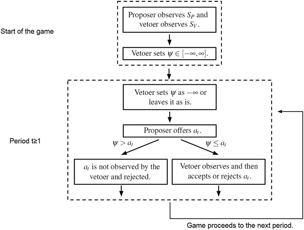
Game tree for the extended model.

In specifying the threshold, ψ, I am modeling a situation where the veteor can decide to impose conditions what proposals she will consider and announce it but has difficulty adjusting these conditions once they are announced. For instance, in negotiating a labor contract, the labor union may announce that it will not accept any wage lower than $10 per hour. The actual negotiation would be handled by a union leader who repeats in every meeting that she does not have the authority to accept any offer below $10 and that any proposal given to her below $10 will be discarded without being heard or read. If the firm attempts to bargain with the members of the union directly, the members could say that they have entrusted bargaining process to the union leader and they will not bargain directly. Such a situation would correspond to setting ψ = 10 initially and sticking to it.

To rescind the announcement, the union can remove the leader and communicate with the proposing firm directly or retract the announcement. By doing so, the union will hear any proposal the proposing firm makes. However, setting a new consequential threshold different from the previous one may be problematic. Suppose the union leader claims that she has received a new direction from the union members lowering the threshold for negotiation to $9. Then, the union loses credibility for the claim that because it has entrusted its leader with negotiations and because its members will not listen to any proposals, its leader is the only one the firm can talk to.

Now, firm reasons that the union members are in communication with the leader and do change the terms of the negotiation based on new information. In this case, the members should be able to listen to information from the firm and readjust their demands. Additionally, if the previous statement that no offer will be considered below $10 was in fact wrong, the new statement can be wrong as well. The firm will doubt whether the threshold is more than an empty bluff serving as a negotiation tactic. In such circumstances, changing the threshold may effectively mean the abandonment of all thresholds for the current negotiation and negotiations of future labor contracts. This is because the firm will point out that it established that what the union claims as thresholds are in fact subject to change and will not believe any new consequential threshold.

Furthermore, if the union leader states that she will not accept an offer lower than $10 on one day, lowers this threshold to $9 on the next day and lowers this again to $8 the day after that, she is not setting preconditions for bargaining. She is already bargaining with the firm. This section models preconditions that are set for the duration of a negotiation and not offers by the vetoer.

5.2 Threshold Pooling Equilibria

In the extended model, I will focus on threshold pooling equilibria (TPE). Proposition 6 demonstrated that in general, pooling equilibria do not exist for the basic model. However, the introduction of the threshold, ψ in the extended model allows the vetoer to never accept or listen to offers below the threshold. In the TPEs, this threshold will always be the same regardless of her type. This is the key characteristic of the TPEs.

In an RTE or an RAE, the bargaining progress demonstrated that the proposer can acquire deals favorable to him using his ability to make offers and bargain down the vetoer. In the TPE, because the vetoer sets a minimum offer that she will accept and sticks to it, the proposer lose the ability to bargain down the vetoer. This lost ability includes the proposer’s ability to succeed in brinkmanship as well. Thus, if the TPE leads the proposer to offer and make deals less favorable to him, the vetoer is better off in a TPE compared to an RTE or an RAE.

For the TPE, players’ strategies adhere to the following assumption.

Unlike in Assumption 1 of the RTE and the RAE, in the above assumption, players’ strategies are not dependent on the proposer’s belief about the vetoer’s type. Instead, given the vetoer’s type, the vetoer has the same cut-off point for all periods. For the proposer, his offer for any period is determined by the same fuction whose input are his type and the threshold, ψ that applies to his offer.

Using the above definition, the following definition specifies the strategies in a TPE.

The vetoer’s strategy means that at the start of the game, vetoer sets the threshold, ψ to equal the high type proposer’s type, p _H . Once set, this threshold never changes. From the offers that make through the threshold and are seen by the vetoer, the vetoer accepts any offer equal to or greater than her type, S _V .

In the proposer’s strategy, S _P < ψ is a case where the current threshold is greater than the proposer’s type S _P . In this case, since all offers that make it through the threshold and are accepted give the proposer negative utility, proposer deliberately makes an offer, ψ − 1 that will be rejected without being viewed. The other case, S _P  ≥ ψ means that there exists some offer that makes it through the current threshold and can give the proposer non-negative utility. Here, from offers that make it through, the offer that the proposer makes is the lowest one that still gives the low type vetoer non-negative utility.

Figure 5 demonstrates how the game plays on the equilibrium path for a TPE. The proposer’s offers are in ovals. At the start of the game, the vetoer sets the threshold to be ψ = p _H and never changes it. Because of this, the high type proposer always makes the only offer that makes it through the threshold and gives him non-negative utility which is p _H . The vetoer always accepts this offer. On the other hand, the low type proposer never has any offer that makes it through the threshold and gives him non-negative utility. Thus, he always offers p _H  − 1 which is always rejected without being seen by the vetoer.

Figure 5:

Offers on the equilibrium path in a TPE.

The following theorem states that a TPE exists if the proposer is unlikely to be low type.

In equation (6), f _H (p _H  − v _L ) is the low type vetoer’s expected utility in a period where the proposer faces a threshold of ψ = p _H . p _L  − v _L is the low type vetoer’s expected utility in a period where the proposer faces a threshold of ψ = p _L . Therefore, a TPE exists when the low type vetoer sees a threshold of ψ = p _H at least as desirable as a threshold of ψ = p _L . When the threshold is always at ψ = p _H , it is too high for the low type proposer to make an offer from which the low type can benefit. If the low type vetoer instead always has a threshold of ψ = p _L , she can see offers of ψ = p _L from all types of proposers. Thus, the expected benefit of this deviation is that the low type vetoer can view the offer from the low type proposer. However, the expected cost of this deviation is that the offer from the high type proposer is reduced.

The vetoer understands that the abandonment of the threshold will mean that vetoer gives up the possibility of a good deal for her. Thus, in a TPE, the vetoer keeps the threshold even if the proposer is low type, deals fail and disasters strike. If, contrary to the assumption of the extended model, changing the threshold to a value above −∞ is possible, the vetoer might try to set a new threshold at a level where she might still get positive utility from a deal and the TPE might not hold. In reality, a vetoer whose strategy is akin to the TPE strategy, sets preconditions for a deal and continues to keep commensurate preconditions for future deals until the situation changes so much that how the vetoer acted previously loses predictive power for the new negotiation.

A TPE exists if and only if the expected benefit is weakly greater than the expected cost. For simplicity, I only deal with PBEs where the threshold is ψ = p _H . Although I do not solve for them in this paper, if f _H (p _H  − v _L ) < p _L  − v _L , there might be PBEs where ψ = p _L .

Vetoer’s expected payoff in an TPE is

The vetoer uses her unchanging high threshold to take all the surplus. Therefore, the proposer’s expected payoff is 0.

I will use the above equation to compare the vetoer’s expected payoffs in an TPE, an RAE and a RTE by discussing how the game plays on the equilibrium paths. It is trivial to see that the expected payoff in equation (7) is always greater than the expected payoff for an RAE in equation (5). The expected benefit of a TPE compared to an RAE is that the threshold of ψ = p _H negates the proposer’s first-mover advantage. Unlike in an RAE, the high type proposer can no longer acquire a deal of v _H . This is because any offer below the threshold, ψ = p _H is not seen by the vetoer. Unlike in an RAE, the proposer can not acquire deals that are no better than rejection for the vetoer because the vetoer will not see them.

The expected cost of a TPE compared to an RAE is 0. If the proposer happens to be low type, all of his offers will be rejected without being seen. However, this is not a loss for the vetoer because the low type proposer’s offer is always v _L in the RAE. In the RAE, the low type proposer uses the first-mover advantage to make an offer is no better than nothing for vetoer under the best circumstances.

The expected benefit of a TPE compared to an RTE is twofold. The first is the negation of the first-mover advantage that I have mentioned while comparing the TPE to the RAE. All of the offers the proposer makes in the RTE, v _L , a ̲ and v _H , are rejected without being seen in the TPE. This is because they are below the threshold. So the proposer can no longer acquire deals that the vetoer is indifferent to compared to no deal. The threshold also means brinkmanship cannot succeed and will not happen in a TPE. In the TPE, the high type proposer offers p _H which is greater than any of the offers in a RTE.

Secondly, the proposer’s information about the vetoer becomes useless to him in a TPE. Any offer the proposer makes below the threshold is not seen. Therefore, even if the proposer knows the vetoer’s type, making different offers based on the vetoer’s type like in a RTE is useless. Offers are made at the threshold level unless the proposer sees no offer that both players would accept.

The expected cost of an TPE compared to an RTE is that if both players are low types, there is no longer a deal in period 1. In an RTE, for the same case, the deal of a ̲ is made. The expected cost is caused by the disappearance of brinkmanship and its leading offer. Given that brinkmanship is the proposer’s strategy to gain information about the vetoer to make lower offers, it is counterintuitive that disappearance of brinkmanship has an expected cost to the vetoer. However, in an RTE, it is not only the high type proposer that makes the brinkmanship’s leading offer of a ̲ in period 1. The low type proposer also makes the same offer. For the brinkmanship to have a chance to succeed, the proposer needs to make the same leading offer for both of his types. Making the same offer sets up the vetoer to think that he could be low type when he is actually high type. In a TPE, brinkmanship and this payment made by the low type proposer for a successful brinkmanship, no longer exists.

6.1 Brinkmanship Failure

Schelling (1981, p. 91, 105) states that limited war can also be a form of brinkmanship when it increases the risk of a major war. A prominent case where brinkmanship failed is President Nixon’s application of the “Madman Theory” to the Vietnam War. The “Madman Theory” was a game theory based approach. According to his chief of staff, H. R. Haldeman, Nixon said the following.

I call it the Madman Theory, Bob. I want the North Vietnamese to believe I’ve reached the point where I might do anything to stop the war. We’ll just slip the word to them that, ‘for God’s sake, you know Nixon is obsessed about Communism. We can’t restrain him when he’s angry–and he has his hand on the nuclear button’–and Ho Chi Minh himself will be in Paris in two days begging for peace.^[14]

On Nixon, Defense Secretary Melvin Laird said “… he wanted adversaries to have the feeling that you could never put your finger on what he might do next.”

During the Vietnam War, the theory was applied by warning the North Vietnamese that if no major progress was made in the peace talks by November 1st of 1969, U.S. will be compelled to “take measures of the greatest consequence.” In October, the Soviet ambassador, Anatoly Dobrynin met with Nixon. Dobrynin reported to the Kremlin that Nixon said “he will never (Nixon twice emphasized that word) accept a humiliating defeat or humiliating terms.” Dobrynin warned the Soviets that “It was perfectly clear from the conversation with Nixon that events surrounding the Vietnam crisis now wholly preoccupy the U.S. President. … Apparently, this is taking on such an emotional coloration that Nixon is unable to control himself even in a conversation with a foreign ambassador.” In the same month, for three days, U.S. had nuclear-armed B-52s test the Soviet defenses, dancing around the edges of the country. However, these signals and actions did little to progress the peace talks.^[15]

Putin’s actions during the Russian invasion of Ukraine such as the transfer of Nuclear weapons to Belarus have also been interpreted as an application of the “Madman Theory”. Also, like the Vietnam War, this war can also be seen as brinkmanship. Putin’s actions and this war have not lead to a deal in the war.^[16]

As stated earlier, debt limit fights and government shutdown fights are common in the United States and for these fights if a deal is not reached, a disastrous effect on the U.S. economy takes place. Most of these fights end with a deal that only changes the status quo slightly.^[17] For example, the 2018–2019 government shutdown was the longest in the U.S. Trump started it when Democrats refused to fund a wall along the U.S.-Mexico border. This shutdown ended in a deal that did not fund this wall.^[18]

One case where a government shutdown initially seemed to have resulted in a deal that changes the status quo meaningfully is the 2011 debt ceiling deal. This deal established budget caps on how much the government can spend. It also created a “supercommittee” which was supposed to come up with a deficit reduction deal. As an incentive for the committee to come up with a deficit reduction deal, the debt ceiling deal stated that unless the deficit reduction deal is passed by congress, sequestration will happen where across-the-board spending cuts take place. These cuts were split evenly between domestic and defense programs and were disastrous for both parties.^[19] The supercommittee failed to reach a deal. Sequestration was delayed and then it took place in March 2023. However, in the same year, a congressional deal succeeded in providing “sequester relief” which reduced the cuts. Also, the budget caps were repeatedly raised allowing the government to spend more money.^[20]

Assuming that both parties are rational, the reason that brinkmanship fails may be explained by the basic model of this paper. In the RTE, once the vetoer succumbs to brinkmanship, the proposer realizes that the vetoer is “weak” (low type) and will succumb to brinkmanship again in the future. This leads to worse offers from the proposer in the future. Because of this, the vetoer who is not “weak” (medium or high type) rejects the brinkmanship offer.

If the party engaging in brinkmanship is irrational, brinkmanship will likely fail in reality. An irrational proposer may demand unrealistically too much from the vetoer. Also, an irrational proposer may not honor deals. In this case, the vetoer should not make concessions to get an unreliable deal.^[21] Finally, if a proposer does not rationally consider deals, the vetoer should make nominal concessions instead of material concessions.

For some of the examples of brinkmanship I have listed, people who were subject to brinkmanship stated or hinted less rigorously similar reasons for not succumbing to brinkmanship.^[22] For the Russian invasion of Ukraine, Ukrainian President Zelenskyy insinuated that making concessions for someone who repeatedly engages in brinkmanship or whose promise is unreliable will lead to bad outcomes.^[23] During the 2018–2019 government shutdown, House Speaker Nancy Pelosi said that if Trump got what he wanted though the shutdown, he will continue to apply the strategy for future demands as well.^[24]

In reality, a vetoer may be unsure whether the proposer is bluffing as Nixon was during the Vietnam war or will actually cause a disaster. If he is bluffing, the vetoer should not succumb to it since the disaster will not materialize. If he is not bluffing, the aforementioned reasons for not succumbing to brinkmanship still apply. So the vetoer should still not succumb.

6.2 Brinkmanship Success

Lemma 1 shows some necessary conditions for the existence of an RTE. From it, I deduce necessary conditions for the success of brinkmanship. First, early brinkmanship cannot be too unfavorable for the vetoer. In Lemma 1, v L + f H δ V 1 − δ V ( v H − v L ) ≤ a ̲ imposes the condition that the brinkmanship offer, a ̲ , is high enough that the low type vetoer deems it worth the cost of succumbing to brinkmanship. Second, similarly, the vetoer needs to be okay with the long term consequences of succumbing to brinkmanship. This may mean that the vetoer is myopic (low δ _V ) or that the future harm from succumbing to brinkmanship is small (low v _H  − v _L ). Lastly, the vetoer needs to believe that because of the proposer’s situation that the proposer likely finds a favorable offer for the vetoer unacceptable (low f _H ).

Russia was involved in the First and Second Chechen Wars, the Russo-Georgian War, the Syrian civil war and the Russian invasion of Crimea. From those wars, Russia and Putin may have learnt that the west is unwilling to risk its relationship with Russia by seriously confronting Russia. This may have lead to Russia’s involvement in more wars and the Russian invasion of Ukraine.^[25] Russia seems to fulfill at least the first two necessary conditions for the success of brinkmanship. It is unclear whether the last condition is fulfilled. First, given the high costs of a breakdown in relationships or war with Russia, the west may have seen losses suffered by other nations to be acceptable. Second, the west may have placed more value on the long term benefits of a favorable relationship with Russia compared to the losses of other nations.^[26]

While we do see cases where brinkmanship succeeds in reality, such cases seem rare and satisfying the necessary conditions for success like those in Lemma 1 seem difficult. Countries, political parties and firms and unions have long term relations they care about. Usually, they will be unwilling to accept the long term consequences of succumbing to brinkmanship. This unwillingness violates the second condition. The last condition means that the vetoer must believe that a better deal for the vetoer is likely to be unacceptable for the proposer. However, in many cases, the vetoer would know that this is false because going back to the status quo before the brinkmanship should be acceptable to both parties. For instance, in a limited war, it is hard to argue that nations would find going back to the status quo before the war unacceptable. For strikes, both the firm and the union are informed about inflation, cost of living, profitability and so on. Therefore, both sides know that a deal in line with these measures should be acceptable to both.

6.3 The Effect of Preconditions on Bargaining

Imposing preconditions on negotiations or the advance of negotiations happens frequently in reality. For instance, consider the Israel-Palestine peace negotiations during the Obama administration. In negotiating the renewal of direct talks with Israel, Palestinian President Mahmoud Abbas had many demands. He demanded a total Israeli settlement freeze. He asked that talks be based on the 1967 lines. He requested the release of 104 Palestinians. He was able to get some prisoners released in return for suspending the Palestinian campaign for U.N. During the ensuing peace talks, a Israeli representative insisted that Israel never place any map on the table till the security conditions were settled. Eventually, the talks failed.^[27] During the Russian Invasion of Ukraine, Ukrainian President Zelenskyy announced that Russia must pull back its troops to where they were before the invasion ere negotiations resumed.^[28]

TPEs demonstrate that sticking to preconditions (the threshold in the extended model) can increase the vetoer’s payoff and that preconditions can be an effective response to brinkmanship. Imposing preconditions is different from brinkmanship. When engaging in brinkmanship, the proposer is flexible. Based on whether the vetoer succumbs to brinkmanship, the proposer changes the subsequent offers. However, the vetoer who imposed preconditions never deviates from them. Therefore, not flexibility but steadfastness is required.

Furthermore, while a proposer engaging in brinkmanship makes an offer that may be unacceptable and has a risk of failure, a vetoer sets preconditions that she thinks are likely to be accepted. An acceptable precondition might be a return to the status quo. This is because walking away from brinkmanship is expected to happen frequently but that walking away from preconditions is not expected to happen. Since this vetoer will not try something different when the preconditions don’t work, she tries to set preconditions that will lead to a deal.

In the basic model, high cut-off points fail because if the vetoer examines all offers, the proposer is going to try the make the worst offer the vetoer will accept. Therefore, to have preconditions that are likely to work, the vetoer must commit to not examining any offer that does not meet the preconditions. This allows her to be steadfast in her preconditions. The vetoer must convince the proposer that this commitment is solid. Bargaining on the strictness of preconditions negates the commitment to the preconditions. In reality, commitment may involve refusing to talk about anything else and refusing to read documents until preconditions are agreed upon. Also, the vetoer could leave the negotiations to representatives who are the only people to talk to and who argue they are not allowed to negotiate preconditions.

References

Acharya, Avidit, and Edoardo Grillo. 2015. “War with Crazy Types.” Political Science Research and Methods 3 (2): 281–307. https://doi.org/10.1017/psrm.2014.23.Search in Google Scholar
Ali, S. Nageeb, Navin Kartik, and Andreas Kleiner. 2023. “Sequential Veto Bargaining with Incomplete Information.” Econometrica 91 (4): 1527–62. https://doi.org/10.3982/ecta20658.Search in Google Scholar
Asselin, Pierre. 2002. A Bitter Peace: Washington, Hanoi, and the Making of the Paris Agreement. The University of North Carolina Press.Search in Google Scholar
Barrett, Ted, Dana Bash, Kate Bolduan, Annalyn Censky, Tom Cohen, Candy Crowley, et al.. 2011. “Debt Ceiling: Timeline of Deal’s Development.” CNN (August 2, 2011). http://www.cnn.com/2011/POLITICS/07/25/debt.talks.timeline/index.html (accessed May 13, 2024).Search in Google Scholar
Ben, Birnbaum, and Amir Tibon. 2014. “The Explosive, Inside Story of How John Kerry Built an Israel-Palestine Peace Plan – and Watched it Crumble.” The New Republic (July 20, 2014). https://newrepublic.com/article/118751/how-israel-palestine-peace-deal-died (accessed February 5, 2024).Search in Google Scholar
Bresnahan, John, and Jake Sherman. 2013. “Budget Agreement Reached.” POLITICO (December 10, 2013). https://www.politico.com/story/2013/12/budget-deal-update-patty-murray-paul-ryan-100960 (accessed May 13, 2024).Search in Google Scholar
Bresnahan, John, Jennifer Scholtes, and Caitlin Emma. 2019. “Sweeping Budget Deal Passes House Despite Weak GOP Support.” POLITICO (July 25, 2019). https://www.politico.com/story/2019/07/25/house-gop-budget-vote-1433848 (accessed May 13, 2024).Search in Google Scholar
Cadelago, Christopher. 2018. “Trump Owns the Shutdown. And He’s OK with that.” POLITICO (December 23, 2018). https://www.politico.com/story/2018/12/23/government-shutdown-2018-trump-white-house-1074565 (accessed May 11, 2024).Search in Google Scholar
Calabuig, Vicente, and Gonzalo Olcina. 2000. “Commitment and Strikes in Wage Bargaining.” Labour Economics 7 (3): 349–72. https://doi.org/10.1016/s0927-5371(00)00002-6.Search in Google Scholar
Cameron, Charles M. 2000. Veto Bargaining: Presidents and the Politics of Negative Power. Cambridge University Press.10.1017/CBO9780511613302Search in Google Scholar
Chambers, Francesca, and Zac Anderson. 2025. “Donald Trump Revives ‘Tough’ Approach to Iran, Warns against Nuclear Weapon.” USA Today (February 4, 2025). https://www.usatoday.com/story/news/politics/2025/02/04/donald-trump-taking-aggressive-approach-iran/77557208007/ (accessed July 27, 2025).Search in Google Scholar
Cheung, Francis K., and Carl Davidson. 1991. “Bargaining Structure and Strike Activity.” Canadian Journal of Economics: 345–71. https://doi.org/10.2307/135627.Search in Google Scholar
Cuellar, Pablo, and Lucas Rentschler. 2023. Threat, Commitment, and Brinkmanship in Adversarial Bargaining. Working Paper.Search in Google Scholar
Detsch, Jack, and Robbie Gramer. 2024. “Russia’s Nuclear Weapons are Now in Belarus.” Foreign Policy (March 14, 2024). https://foreignpolicy.com/2024/03/14/russia-nuclear-weapons-belarus-putin/ (accessed May 13, 2024).Search in Google Scholar
Drawbaugh, Kevin, Donna Smith, Thomas Ferraro, and Dave Clarke. 2011. “Factbox: Top Contenders for Budget/Tax Super Committee.” Reuters (August 4, 2011). https://www.reuters.com/article/us-usa-debt-committee-idUSTRE7733FC20110804/ (accessed May 13, 2024).Search in Google Scholar
“FACTBOX: Facts about the 2008 War in Georgia.” 2009. Reuters (August 4, 2009). https://www.reuters.com/article/idUSTRE5732TH/ (accessed May 17, 2024).Search in Google Scholar
Fanning, Jack. 2016. “Reputational Bargaining and Deadlines.” Econometrica 84 (3): 1131–79. https://doi.org/10.3982/ecta12628.Search in Google Scholar
Fearon, James D. 1994. “Domestic Political Audiences and the Escalation of International Disputes.” American Political Science Review 88 (3): 577–92. https://doi.org/10.2307/2944796.Search in Google Scholar
Fudenberg, Drew, and Jean Tirole. 1983. “Sequential Bargaining with Incomplete Information.” The Review of Economic Studies 50 (2): 221–47. https://doi.org/10.2307/2297414.Search in Google Scholar
Fudenberg, Drew, and Jean Tirole. 2005. Game Theory. Ane Books Pvt. Ltd.Search in Google Scholar
Fudenberg, Drew, David Levine, and Jean Tirole. 1985. “Infinite-horizon Models of Bargaining with One-Sided Incomplete Information.” In Game-Theoretic Models of Bargaining, edited by Alvin E. Roth, 73–98. Cambridge University Press.10.1017/CBO9780511528309.006Search in Google Scholar
Gibbons, Robert. 1992. Game Theory for Applied Economicsts. Princeton University Press.10.1515/9781400835881Search in Google Scholar
Golshan, Tara. 2018. “Congress’s Massive Budget Deal, Explained.” Vox (February 7, 2018). https://www.vox.com/policy-and-politics/2018/2/7/16987122/congress-massive-budget-deal-explained (accessed May 13, 2024).Search in Google Scholar
Graf, Garrett M. 2017. “The Madman and the Bomb.” POLITICO (August 11, 2017). https://www.politico.com/magazine/story/2017/08/11/donald-trump-nuclear-weapons-richard-nixon-215478/ (accessed May 7, 2024).Search in Google Scholar
Ha, Yong Chool, and Chaesung Chun. 2010. “North Korea’s Brinkmanship and the Task to Solve the “Nuclear Dilemma”.” Asian Perspective 34 (1): 87–109. https://doi.org/10.1353/apr.2010.0033.Search in Google Scholar
Haberkorn, Jennifer, Jonathan Lemire, and Sam Stein. 2023. “White House Prepares to Fight for Ukraine Aid after Shutdown Averted.” POLITICO (September 30, 2023). https://www.politico.com/news/2023/09/30/biden-administration-congress-government-shutdown-deal-ukraine-aid-00119296 (accessed May 11, 2024).Search in Google Scholar
Haldeman, H. R., and Joseph DiMona. 1978. The Ends of Power. Times Books.Search in Google Scholar
Hart, Oliver D., and Jean Tirole. 1988. “Contract Renegotiation and Coasian Dynamics.” The Review of Economic Studies 55 (4): 509–40. https://doi.org/10.2307/2297403.Search in Google Scholar
Hayes, Beth. 1984. “Unions and Strikes with Asymmetric Information.” Journal of Labor Economics 2 (1): 57–83. https://doi.org/10.1086/298023.Search in Google Scholar
Hicks, J. R. 1963. The Theory of Wages. Macmillan.10.1007/978-1-349-00189-7Search in Google Scholar
“How Russia’s Grab of Crimea 10 Years Ago Led to War with Ukraine and Rising Tensions with the West.” 2024. Associated Press (March 18, 2024). https://apnews.com/article/russia-putin-ukraine-crimea-seizure-8245aec572fb71236febfa8735c42879 (accessed May 17, 2024).Search in Google Scholar
Hussein, Fatima. 2023. “Why a Government Default Could be Worse than a Government Shutdown.” Associated Press (May 18, 2023). https://apnews.com/article/debt-limit-default-government-shutdown-explainer-b38474f210e519aeb3f48107ca2657ba (accessed April 30, 2024).Search in Google Scholar
“Iran’s Khamenei Says Experience Proves Talks with US ‘Not Smart.” 2025. Reuters (February 7, 2025). https://www.reuters.com/world/middle-east/irans-khamenei-says-experience-proves-talks-with-us-not-smart-2025-02-07/ (accessed February 7, 2025).Search in Google Scholar
Jacobson, Zachary Jonathan. 2023. “The Lesson of Richard Nixon for Interpreting Putin’s Saber Rattling.” Washington Post (April 7, 2023). https://www.washingtonpost.com/made-by-history/2023/04/07/richard-nixon-vladimir-putin-nuclear/ (accessed May 13, 2024).Search in Google Scholar
Jacod, Jean, and Philip Protter. 2005. Probability Essentials. Springer-Verlag.10.1007/978-3-642-55682-1Search in Google Scholar
Kennan, John. 1986. “The Economics of Strikes.” In Handbook of Labor Economics, Vol. 2, edited by Orley C. Ashenfelter, and Richard Layard, 1091–137.10.1016/S1573-4463(86)02009-6Search in Google Scholar
Kim, Seungryeon. 2023. “[Ramble/Kim Seungryeon]Putin’s “Madman” Strategy … Nuclear-Powered Cruise Missile Development.” Dong-a Ilbo (October 10, 2023). https://www.donga.com/news/Opinion/article/all/20231008/121572449/1 (accessed March 12, 2025).Search in Google Scholar
Kosnar, Mike, and Andrew Rafferty. 2013. “Border Protection Workers Warned of Possible Furloughs Due to Sequester.” NBC News (March 7, 2013). https://www.nbcnews.com/news/us-news/border-protection-workers-warned-possible-furloughs-due-sequester-flna1c8760981 (accessed May 13, 2024).Search in Google Scholar
Kwong, Matt. 2019. “Trump’s Greatest Shutdown Challenge, thy Name is ‘Nancy’.” Canadian Broadcasting Corporation (January 25, 2019). https://www.cbc.ca/news/world/donald-trump-nancy-pelosi-congress-1.4992178 (accessed April 30, 2024).Search in Google Scholar
Lee, Janghun. 2022. “Putin’s Madman Strategy, a Scheme to End the Ukraine War?” Dong-a Ilbo (October 1, 2022). https://www.donga.com/news/Inter/article/all/20221001/115749169/1 (accessed May 13, 2024).Search in Google Scholar
Matthews, Dylan. 2013. “The Sequester: Absolutely Everything You Could Possibly Need to Know, in One FAQ.” Washington Post (February 20, 2013). https://www.washingtonpost.com/news/wonk/wp/2013/02/20/the-sequester-absolutely-everything-you-could-possibly-need-to-know-in-one-faq/ (accessed May 13, 2024).Search in Google Scholar
Mauro, Martin J. 1982. “Strikes as a Result of Imperfect Information.” Industrial and Labor Relations Review 35 (4): 522–38. https://doi.org/10.2307/2522665.Search in Google Scholar
Mazalan, Ricardo. 2022. “Zelensky Demands Russian Troops Leave Ukraine as Precondition to Diplomacy.” The Times of Israel (May 25, 2022). https://www.timesofisrael.com/zelensky-demands-russian-troops-leave-ukraine-as-precondition-to-diplomacy/ (accessed April 28, 2024).Search in Google Scholar
Megerian, Chris. 2023. “Biden Signs Debt Ceiling Bill that Pulls US Back from Brink of Unprecedented Default.” Associated Press (June 3, 2023). https://apnews.com/article/joe-biden-debt-ceiling-budget-signing-f78a000d83cf85ffbaa2d08637844053 (accessed May 11, 2024).Search in Google Scholar
Mroue, Bassem. 2023. “Russian Fighter Jets Harass American Drones over Syria, US Military Says.” Associated Press (July 8, 2023). https://apnews.com/article/syria-russia-us-drones-827cd57a36ef5b775d30e77f6b07ec1e (accessed May 17, 2024).Search in Google Scholar
Osborne, Martin J. 1985. “The Role of Risk Aversion in a Simple Bargaining Model.” In Game-Theoretic Models of Bargaining, edited by Alvin E. Roth, 181–213. Cambridge University Press.10.1017/CBO9780511528309.010Search in Google Scholar
Parlapiano, Alicia. 2015. “How Congress Has Worked to Avoid the ‘Sequester’ Spending Caps.” The New York Times (October 29, 2015). https://www.nytimes.com/interactive/2015/10/29/us/politics/how-congress-has-worked-to-avoid-the-sequester-spending-caps.html (accessed May 13, 2024).Search in Google Scholar
Pelosi, Nancy. 2019. January 22, 2019. https://twitter.com/TeamPelosi/status/1087908114534461441 (accessed April 30, 2024).Search in Google Scholar
Powell, Robert. 2006. “War as a Commitment Problem.” International Organization 60 (1): 169–203. https://doi.org/10.1017/s0020818306060061.Search in Google Scholar
Powell, Robert. 2015. “Nuclear Brinkmanship, Limited War, and Military Power.” International Organization 69 (3): 589–626. https://doi.org/10.1017/s0020818315000028.Search in Google Scholar
Pratt, John W. 1964. “Risk Aversion in the Small and in the Large.” Econometrica 32 (1–2): 122–36. https://doi.org/10.2307/1913738.Search in Google Scholar
Prokop, Andrew. 2023. “5 Winners and 5 Losers from the Debt Ceiling Deal: Biden and McCarthy Win. The Freedom Caucus Loses.” Vox (June 1, 2023). https://www.vox.com/politics/2023/6/1/23743797/debt-ceiling-biden-mccarthy-winners-losers (accessed May 11, 2024).Search in Google Scholar
Reder, Melvin W., and George R. Neumann. 1980. “Conflict and Contract: The Case of Strikes.” Journal of Political Economy 88 (5): 867–86. https://doi.org/10.1086/260912.Search in Google Scholar
Rennolds, Nathan. 2024. “Bleak Images Show Snapshots of Daily Life in the Closed World of North Korea.” Business Insider (March 24, 2024). https://www.businessinsider.com/bleak-images-show-snapshots-daily-life-north-korea-2024-3 (accessed April 30, 2024).Search in Google Scholar
Restuccia, Andrew, Burgess Everett, and Heather Caygle. 2019. “Longest Shutdown in History Ends after Trump Relents on Wall.” POLITICO (January 25, 2019). https://www.politico.com/story/2019/01/25/trump-shutdown-announcement-1125529 (accessed May 11, 2024).Search in Google Scholar
Roberts, Dan. 2013. “US Congressional Leaders Unveil Two-Year Budget Deal.” The Guardian (December 10, 2013). https://www.theguardian.com/world/2013/dec/10/us-congress-reaches-budget-deal (accessed May 13, 2024).Search in Google Scholar
Robinson, James A. 1999. “Dynamic Contractual Enforcement: A Model of Strikes.” International Economic Review 40 (1): 209–29. https://doi.org/10.1111/1468-2354.00012.Search in Google Scholar
Romer, Thomas, and Howard Rosenthal. 1978. “Political Resource Allocation, Controlled Agendas, and the Status Quo.” Public Choice: 27–43. https://doi.org/10.1007/bf03187594.Search in Google Scholar
Roth, Alvin E. 1985. “A Note on Risk Aversion in a Perfect Equilibrium Model of Bargaining.” Econometrica: Journal of the Econometric Society: 207–11. https://doi.org/10.2307/1911733.Search in Google Scholar
Roth, Alvin E. 1989. “Risk Aversion and the Relationship between Nash’s Solution and Subgame Perfect Equilibrium of Sequential Bargaining.” Journal of Risk and Uncertainty 2 (4): 353–65. https://doi.org/10.1007/bf00356861.Search in Google Scholar
Rubinstein, Ariel. 1982. “Perfect Equilibrium in a Bargaining Model.” Econometrica: 97–109. https://doi.org/10.2307/1912531.Search in Google Scholar
Santaliz, Kate, Thorp V. Frank, and Rebecca Shabad. 2023. “Senate Confirms 425 Military Nominees after Sen. Tommy Tuberville Drops His Hold.” NBC News (December 5, 2023). https://www.nbcnews.com/politics/congress/sen-tommy-tuberville-drops-hold-hundreds-military-nominees-rcna128138 (accessed April 30, 2024).Search in Google Scholar
Schaul, Kevin, and Kevin Uhrmacher. 2024. “The Shortest and Longest Government Shutdowns in U.S. History.” Washington Post (March 19, 2024). https://www.washingtonpost.com/politics/2023/longest-government-shutdown/ (accessed May 28, 2024).Search in Google Scholar
Schelling, Thomas C. 1967. Arms and Influence. Yale University Press.10.2307/j.ctt5vm52sSearch in Google Scholar
Schelling, Thomas C. 1981. The Strategy of Conflict. Harvard University Press.Search in Google Scholar
Schmidt, Klaus M. 1993. “Commitment through Incomplete Information in a Simple Repeated Bargaining Game.” Journal of Economic Theory 60 (1): 114–39. https://doi.org/10.1006/jeth.1993.1037.Search in Google Scholar
Scholtes, Jennifer, and Caitlin Emma. 2023. “The Debt-Limit Time Machine: What the Last 10 Big Fights Tell Us about this One: A Decade Filled with Fiscal Standoffs Shows us Three Telling Truths about How Congress and the White House Might Handle the Current Impasse – No DeLorean Needed.” POLITICO (March 6, 2023). https://www.politico.com/news/2023/03/06/debt-limit-flashbacks-00085493 (accessed May 11, 2024).Search in Google Scholar
Schwarz, Michael, and Konstantin Sonin. 2008. “A Theory of Brinkmanship, Conflicts, and Commitments.” Journal of Law, Economics, and Organization 24 (1): 163–83. https://doi.org/10.1093/jleo/ewm038.Search in Google Scholar
Shin, David W. 2020. Kim Jong-Un’s Strategy for Survival: A Method to Madness. Lexington Books.10.5771/9781793608215Search in Google Scholar
Skaperdas, Stergios. 2006. “Bargaining versus Fighting.” Defence and Peace Economics 17 (6): 657–76. https://doi.org/10.1080/10242690601025617.Search in Google Scholar
Slantchev, Branislav L. 2003. “The Principle of Convergence in Wartime Negotiations.” American Political Science Review 97 (4): 621–32. https://doi.org/10.1017/s0003055403000911.Search in Google Scholar
Smith, Steve, Amelia Hadfield, and Tim Dunne, eds. 2008. Foreign Policy: Theories, Actors, Cases. Oxford University Press.Search in Google Scholar
Snyder, Scott. 2001. “Patterns in North Korea’s Diplmatic Style.” In Korea in the 21st Century, edited by Seung-Ho Joo, and Tae-Hwan Kwak, 107–29. Nova Science Publishers.Search in Google Scholar
Tani, Shotaro, and Alice Hancock. 2024. “EU Drop in Russian Gas Imports Raises Hopes of Energy Independence.” Financial Times (January 4, 2024). https://www.ft.com/content/46d2f5a7-37ab-4196-bd00-754b9dfe7fb0 (accessed May 18, 2024).Search in Google Scholar
Tracy, Joseph S. 1984. “A Theoretical and Empirical Investigation of U.S. Strike Activity.” Ph.D. diss. The University of Chicago.Search in Google Scholar
US. 2018. “US Shutdown: Democrats Refuse Funds for Trump Wall.” BBC (December 17, 2018). https://www.bbc.com/news/world-us-canada-46596272 (accessed May 11, 2024).Search in Google Scholar
What to Read to Understand Chechnya. 2024. The Economist (April 16, 2024). https://www.economist.com/the-economist-reads/2024/04/16/what-to-read-to-understand-chechnya (accessed May 17, 2024).Search in Google Scholar
Yglesias, Matthew. 2013. “The Idiocy of Sequestration.” Slate (January 30, 2013). https://slate.com/business/2013/01/what-is-sequestration-the-budget-cuts-will-slam-government-spending-yet-not-fix-our-real-budget-problems.html (accessed May 13, 2024).Search in Google Scholar
Zakaria, Fareed. 2023. “Exclusive Interview with Ukrainian President Volodymyr Zelensky on the Counteroffensive, Putin, and Corruption in Ukraine.” CNN (September 10, 2023). https://www.cnn.com/audio/podcasts/fareed-zakaria-gps/episodes/39107018-f7a5-494c-8a23-b079013bd1b2 (accessed May 7, 2024).Search in Google Scholar
Supplementary Material
This article contains supplementary material (https://doi.org/10.1515/peps-2025-0020).
© 2025 the author(s), published by De Gruyter, Berlin/Boston
This work is licensed under the Creative Commons Attribution 4.0 International License.
Articles in the same Issue
- Frontmatter
- Research Articles