Three-dimensional spatiotemporal tracking of nano-objects diffusing in water-filled optofluidic microstructured fiber

1 Introduction

Measuring the trajectory of diffusing nano-objects that have dimensions substantially below the diffraction limit represents a powerful approach particular within bioanalytics and life science. This allows us to understand processes at the nanoscale level, examples of which include protein folding [1] or for measuring virus concentrations [2]. Various types of microscopy-based image processing techniques for object localization and tracking with both high temporal resolution, as well as localization precision have been developed [3], [4]. However, most currently employed schemes only track the object of interest in the image plane, while accessing the axial dimension, i.e., conducting full three-dimensional (3D) tracking, is considerably more challenging. Promising experiments using multifocal plane microscopy [5] or point spread function engineering [6], [7] have been conducted, while standard microscopes cannot be directly used due to the need for additional components (e.g., additional camera [8], phase masks [9]).

Recently microstructured optical fibers have been introduced as a novel platform for the tracking of diffusing nano-objects over very long time scales using elastic light scattering [9], [10], [11], [12], [13]. Here tracking by means of elastic light scattering includes key advantages such as unlimited photon budget, fast data acquisition [14], [15] and avoidance of labeling [16], all of which are difficult to achieve with fluorescence-based schemes. As recently demonstrated, one configuration of the fiber-based approach allows full 3D tracking of a diffusing nanosphere over thousands of frames at kHz frames rates via elastic light scattering–based position retrieval [13]. This approach uses a microstructured optical fiber including a liquid-filled microchannel (diameter D^m ≈ 1 µm) running parallel to the light guiding glass core (with a center-to-center distance of about 2 µm) allowing to retrieve the position of the nano-object along the direction of the microscopic detection via the intensity of the light scattered at the evanescent field of the core mode. Specifically, the successful tracking of a diffusing 50-nm gold nanosphere along all three spatial directions over seconds was demonstrated. Particular remarkable is the very large number of continuously recorded frames (N_f = 8000) greatly exceeding the track lengths of other reported evanescent-based 3D tracking schemes, examples of which include the tracking of 200 nm polystyrene sphere nanoparticles inside water (N_f = 67) [17] or nil red molecules inside poly(acrylamide) (PAA) gel (N_f = 8) [18]. Here is it important to note that as the standard deviation of the determined diffusion coefficient scales with 1/Nf [19], [20], [21], the fiber-based approach shows an unprecedented statistical significance regarding the determination of hydrodynamic diameters. Compared to commonly used nanoparticle tracking analysis (NTA), which due to low number of frames gives a precision (i.e., standard deviation) per ensemble, the fiber approach yields a very high precision per nano-object. This allows for principally studying the dynamics of single nano-objects, an issue that is challenging to achieve with the commonly used implementations of NTA. Other advantages of the fiber approach include high and homogeneous illumination intensity along the entire field of view (i.e., diffractionless light-line illumination), confinement of the nano-objects to the area of illumination and the focal plane of the microscope, reduced readout time and increased frame rates due to the smaller imaging window (35 pixel height) on the camera chip, principal compatibility with fiber circuitry, very small sample volumes (<200 pL) and, in contrast to fluorescence, no photodegradation.

In spite of these benefits mentioned above, this fiber-based 3D tracking approach demands a specific value of refractive index (RI) inside the microchannel to achieve an exponential evanescent field and an unambiguous correlation between scattered intensity and position. Such RI adjustment has been achieved using a composite liquid containing water and dimethyl sulfoxide (DMSO), although the use of a mixture is unfavorable for bioanalytical applications typically requiring a water environment.

In this work, we resolve the mentioned issue by an extended data processing procedure of the measured trajectories, allowing for 3D tracking inside a half semicircle region of the microchannel of the optofluidic fiber in case it is filled with water (Figure 1a). The hydrodynamic diameter of the nanosphere within the confined channel is estimated by applying the resistance coefficient for the three directions separately. The presented 3D tracking approach includes all mentioned advantages of fiber-based 3D tracking and additionally is able to handle a water environment, making this system in particular relevant for bioanalytics applications.

Figure 1:

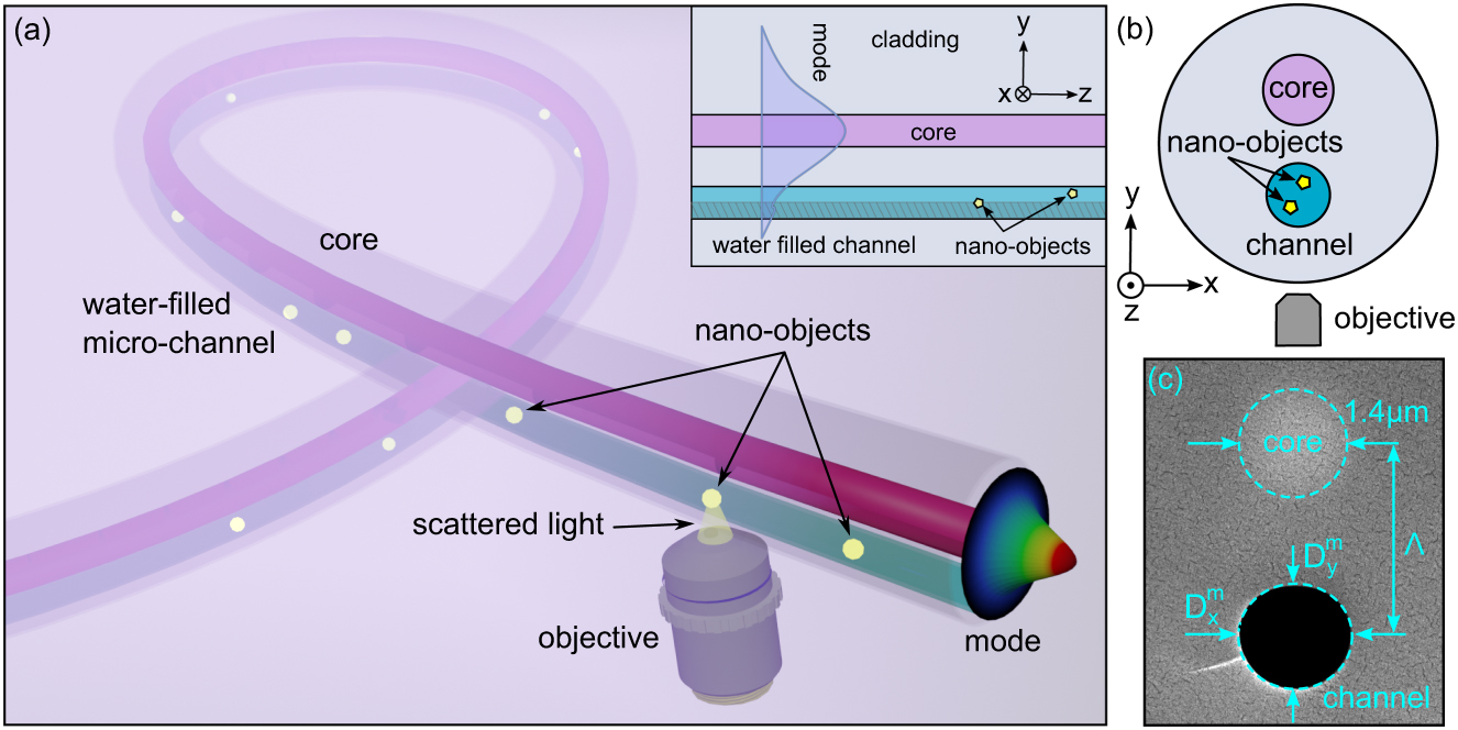
The concept of three-dimensional (3D) tracking of nano-objects inside a water-filled modified graded index fiber. (a) Illustration of the concept (light blue: water-filled microchannel, red: optical core). The yellow elements represent the nano-objects. The inset is a sketch of the fiber cross-section within the yz-plane showing the modal intensity distribution of the core mode along the y-direction. The intensity based y-position retrieval can be achieved in the highlighted channel region (nondashed area). (b) Sketch of fiber cross-section (xy-plane) and experimental configuration (i.e., relative orientation of core, microchannel and microscope objective) used for 3D tracking. (c) Scanning electron micrographic (SEM) image of the cross-section of the implemented microstructured fiber.

2 Concept and working principle

The working principle of the waveguide-based 3D tracking scheme discussed here relies on a combination of localization microscopy within the image plane (xz-plane, Figure 1a inset) and scattering light–based position retrieval along axial direction (y-direction, Figures 1b and 1a inset).

The waveguide used is a microstructured single-mode graded index fiber (MGIF) (Figure 1a) consisting of a central waveguide core with a longitudinal water-filled microchannel (diameter Dm≈1 μm) running parallel to the glass core. The nano-objects diffusing inside the water-filled microchannel are homogenously illuminated by the evanescent field inside the channel across the entire field of view. They are localized within the image plane via the elastically scattered light that is sidewise detected by a microscope. The position of the particle along y-direction can be retrieved from the scattered intensity due to the relation between the y-coordinates and local field intensity I = I(y). Therefore, this special fiber geometry provides a platform for 3D tracking by retrieving the depth location (y-axis) from the scattered intensity which commonly cannot be measured. The position within the xz-plane is determined by image processing, i.e., via center-of-mass analysis in the recorded images.

In order to decode the axial position from the scattered intensity, an bijective function between the local intensity distribution of the evanescent field and the y-coordinate (I = f(y), y = f⁻¹(I)), (f⁻¹ is the reverse of f) is required, i.e., the y-position can be uniquely determined from one certain intensity. In contrast to the water-DMSO mixture used in our previous work (RI n_r = 1.44 at a wavelength of λ = 640 nm) [13], in which the field intensity can be described by a uniform exponential function within the whole channel, the intensity distribution (simulated by finite-element modeling using COMSOL) of the evanescent field inside the microchannel in case of pure water filling is substantially more complex regarding the following three aspects: (i) First, using water leads to a distinct variation of the intensity inside the microchannel not only along the y-axis but also along the x-direction in contrast to our previous work using DMSO/water. Consequently, the mathematical function that relates y-position and intensity must be determined separately for each x-position. (ii) Secondly, the function between intensity and y-position is surjective (i.e., double-valued) at certain x-positions within a certain part of the low-intensity region (red-shaded area in Figure 2a), yielding an irreversibility from intensity to y-position. Therefore, the intensity position recovery can only be achieved exclusively in the single-valued region of the channel (nonred-shaded area in Figure 2a). (iii) Another feature is the nonexponential decay of the evanescent field for each x-position particular in the low-intensity semicircle of the microchannel (meshed area in Figure 2a). Here the deviation from a single exponential decay is significant in contrast to the upper semicircle (Figure 2c).

Figure 2:

(a) Simulated spatial intensity distribution (logarithmic color scale including iso-intensity contour lines) in a circular water-filled microchannel (diameter Dm=1 μm,λ=642 nm). The correlation between the local field intensity and the y-coordinates is ambiguous in the red-shaded area and position retrieval is performed in the upper semicircle. (b) Close-up of the intensity distribution in the upper semicircle of the microchannel The white vertical lines indicate the boundaries between the adjacent bins along the x-direction. In each bin, the highest scattered intensity occurs when the particle is at the upper channel wall indicated by y_max (center of the particle). The median scattered intensity is expected to be at y_med = 0 (see text for details). (c) Intensity distribution along the y-direction of selected bins in case of 100 bins partitioning (bin width 10 nm). Exponential fitting is applied to the points in the upper semicircle (nonhashed area) for each bin, representing by the dashed curves in corresponding darker colors.

In order to circumvent the mentioned issues, the 3D tracking addressed here is restricted to the upper semicircle of the microchannel (I = I(x, y ≥ 0), nonmeshed area in Figure 2a and b), i.e., high-intensity region which is partitioned into small bins along x-direction (Figure 2b). This choice yields a bijective (i.e., single-valued) function between intensity and position in each bin. A detailed investigation of the mode field in y-direction within defined spatial bins has revealed that a single exponential function including two parameters can be used to approximate the field behavior in that region (Figure 2c):

with the slope and local intensity parameters p_i = p_i(x) and b_i = b_i(x), respectively, that both depend on the bin index i. Examples of intensity distributions for selected bins including the respective fit using Eq. (1) are shown in Figure 2c, confirming the applicableness of a single exponential function with x-dependent parameters. As a consequence, the locations of a nano-object along the y-direction within the upper semicircle of the microchannel cross section can be retrieved from its scattered intensity bin by bin.

3 Methods

The fiber used in the experiments consists of a graded index GeO₂-doped silica core (1.4 µm diameter) with a maximum RI of n_r = 1.49 (maximum doping concentration is 24 mol %) [22] in the center and a parallel running microchannel with pitch (center-to-center distance) of Λ=2 μm (Figure 1b). The fiber is single-mode at the operation wavelength λ=642 nm. SEM imaging (Figure 1c) reveals that the microchannel is slightly elliptical with the principal extensions along the x- and y-directions of Dxm=1.2 μm and Dym=1.1 μm, respectively.

The solution used consists of water of buffer medium and spherical gold nanoparticles (particle concentration of 5.6 × 10⁹ particles/mL). Prior to the tracking experiment, the diameter distribution of the nanosphere ensemble has been characterized using a commercially available device (Malvern Zetasizer Nano ZS), showing an average hydrodynamic diameter and a standard deviation of dNP¯=104.3 nm and σNP=0.66 nm, respectively. Here we use the z-average as mean nanoparticle diameter, which is typically considered in the literature within the context of Zetasizer measurements, i.e., dynamic light scattering (DLS) experiments. The standard deviation stated has been obtained here from statistically analyzing a series of Zetasizer measurements (here nine) on the same sample. The choice of nanosphere diameter represents a compromise between the intensity decay across the water-filled microchannel, the in-fiber power, the scattering cross section and the frame rate, allowing the nanosphere to be tracked along the transverse direction at any time. The particle diameter considered here is larger compared to our previous work [13], imposed by a smaller scattering coefficient and a faster field decay, both of which result from the smaller RI of water compared to the liquid used in our previous work.

For the tracking experiments, red laser light (Thorlabs HL6366DG, λ=642 nm) is coupled into the fiber core via an objective (20×, NA = 0.4) from one end of the fiber. This solution is introduced into the microchannel from the output side of the fiber by capillary action within several minutes until the respective observation region of the microscope objective is filled with the nano-object solution (a sketch of the experimental setup and a plot of the calculated filling time can be found in the Supplementary material). Note that the required sample volumes are extremely small (<200 pL). In order to avoid the impact of drift the tracking experiment was not started until the liquid flow was vanished. To confirm the absence of flow, the trajectories of the nano-object along z-direction is plotted in Figure 3a, showing no direction-biased movement. The corresponding histogram of the probability of the displacement along the z-direction at different time intervals, as well as the related normal distribution fittings (red curves in Figure 3c) that are centered on the origin further confirming the absence of flow. The sidewise scattered light from the gold nanoparticles (measured at a distance of 7 cm from the output side) is collected by an oil-immersed ×60 objective and imaged onto a sCMOS camera (ANDOR Zyla 4.2 Plus). The raw video of the tracking experiment is presented in the Supplementary material and three selected frames are shown in Figure 3b. Note that for the 3D tracking, the fiber is oriented such that the connection line between the centers of core and microchannel coincides with the axis of the objective (Figure 1b). Within the presented experiments, the guided power in the fiber was about 2.4 mW and the camera frame rate was ν=2741 Hz with the exposure time of 0.36 ms. The input power was chosen on the basis of considering the trade-off between the saturation of signal in the upper semicircle and the detecting the nanoparticle at any location in the lower semicircle.

Figure 3:

Longitudinal trajectory of the single gold nanosphere considered here. (a) Trajectory along z-direction. The three red dots mark the examples of frames which are shown in (b). (b) Selected frames from the tracking video, with the determined position of the particle marked by the yellow dashed circles. The number indicates the frame. (c) Histogram of the probability of the nanosphere displacement along the z-direction at different time intervals. The lines refer to the corresponding normal distribution fitting curves (red curves).

The tracking procedure within the image plane (i.e., xz-plane) involves frame-by-frame center-of-mass localization using the Trackpy (v. 0.3.3) package of Python. As examples, the determined positions of the particle in 2000th, 8000th and 11,000th frames are marked by the yellow dashed circles in Figure 3b. The final result is a data set containing over 10 thousands of entries, each of which includes the x-, z-locations and the corresponding scattered intensity (entry_j = {x, z, I}j with the frame index j). Optimization of the various parameters leads to a transverse localization accuracy of σtr=3.06 nm.

The determination of the parameters required for Eq. (1) mainly requires the two following data processing procedures: (i) partitioning the trajectory along the x-axis in bins and (ii) selection of data entries that are within the upper (high-intensity) semicircle (non-meshed area in Figure 2a). Note that the data processing does not rely on the simulated mode field patterns but rather uses the measured trajectory, thus circumventing the impact of improper knowledge on RI distribution and/or geometric parameters.

4 Results

The spatial distribution of the parameters p and b obtained from the bin-by-bin procedure of the tracked data (red dots) are compared in Figure 4 to corresponding values from simulations using the same data treatment (dashed blue lines). The slope parameter obtained from experiment p_exp shows a very good agreement with its simulated counterpart p_sim (Dx,simm=1.2 μm,Dy,simm=1.1 μm) (Figure 4a) which is remarkable considering that this parameter has been determined from two pairs of values only and that the simulations include several assumptions such as a perfect ellipse shape of the channel or a simple concentric RI distribution in the core. More pronounced deviations are visible at lower bin indices, i.e., positions closer to the boundaries of the microchannel. We attribute this to the lower number of frames available (inset of Figure 4a). Statistically speaking, more frames available within one bin imposes a higher probability that the nano-object is located at y = 0 and y = y_max, thus leading to higher probability to obtain more accurate intensity values at these two positions (I_med,i and I_max,i). Note that another potential source of error is the limited spatial resolution of the SEM imaging impacting the determination of the extension of the channel along the y-direction. Within the context of the analysis presented, the uncertainty in the determination of dym is Δdym=±80 nm, imposing an error in the estimation of y_max with this impact being strongest in the center of the semicircle (x_i = 0). Besides, the non-ideal ellipse shape of the channel also contributes to the error which is not considered in both simulations and experimental data analysis.

Figure 4:

Dependence of (a) slope and (b) local intensity parameters (p and b) on bin index along the x-direction. The cyan dots and the black line refer to the data obtained from the tracked data and the corresponding 2nd order polynomial fit. The red lines result from the finite element simulation. The corresponding number of available frames used in the respective bin N_bin,i is plotted in the inset of (a).

As the parameter b scales with the local field intensity, b_sim can be adapted to the range of b_exp as shown in Figure 4b showing a good agreement in terms of evolution and dynamic range between simulation and experiment.

4.1 3D trajectories recovery

To obtain continuous correlations between the parameters and the x-position (p = p(x) and b = b(x)) independent of simulations, we applied 2nd order polynomial fitting to the experimentally obtained parameters p_i and b_i in each bin with the corresponding central bin position x¯i (black lines in Figure 4a and b). Note that the feasibility of using second order polynomial fitting to the parameters is confirmed in simulations as shown in the Supplementary material. Therefore, the y-position for frame j in the upper half channel region can be retrieved by solving Eq. (1) for y, leading to y_j = (log(I_j(x)) − b(x))/p(x).

Together with the tracked positions in the xz-plane, the frame number–sorted 3D trajectory of the nanoparticle ({x, y, z}_k with entry index of k = 1 … N_up [N_up: number of frames in the upper region]) within the high-intensity semicircle is obtained. The projection of nanoparticle positions onto the xy-plane (fiber cross-section plane) is shown in Figure 5b with 97.23% of retrieved y-positions being located within the upper semicircle. Note that the remaining 2.77% trajectories are out of the upper semicircle due to the polynomial fit used for the parameters of Eq. (1) (Figure 4). The plot reveals an homogenous nanoparticle distribution across the upper semicircle and thus post a priori confirming the assumption that was required to determine I_med,i and I_max,i. The 3D trajectory in the upper semicircle is visualized in Figure 5a, confirming the feasibility of the scattered-intensity–associated 3D tracking approach. Note that once the nanoparticles enters the lower intensity region (y < 0), tracking along the y-direction in not feasible via the use of Eq. (1), i.e., the 3D tracking procedure is only valid in the upper semicircle. To highlight this procedure, Figure 5a shows the continuous parts of the trajectory of the nanosphere that are solely located in the upper semicircle. Here each subtrajectory is shown in one single color. The number of continuous trajectories of the nanoparticle in the upper semicircle is N_con = 492, while the averaged and maximum number of frames per continuous trajectory are N_ave = 16 and N_max = 262.

Figure 5:

Three-dimensional (3D) tracking of a 100 nm gold nanosphere inside the water-filled mode graded index fiber (MGIF). (a) Parts of the 3D trajectory of a single diffusing nanosphere in three spatial dimensions within the upper part of the microchannel (indicated by the semitransparent red background). Note that the position retrieval along the y-direction is only valid within the upper semicircle and therefore only this part is presented in (a). Each color represents a continuous subtrajectory and the color scale refers to relative position of the respective subtrajectory inside the entire track ensemble (e.g., 100% refers to N_con = 492). (b) Transverse locations of the nanoparticle within the upper semicircle of microchannel, i.e., projection of the entire data set onto the xy-plane. The boundaries of channel and center of particle are separately indicted by the red solid and red dash lines. The border between upper and lower half of the channel (y = 0 μm) is illustrated by the blue dashed line. The color of each point refers to the location of the nanoparticles at a specific time.

4.2 Mean squared displacement analysis and Stokes–Einstein relation

One important application of NTA is diameter determination of deep subwavelength nano-objects via mean squared displacement (MSD) analysis [23], [24], [25]. This analysis is associated with the statistical nature of Brownian motion, i.e., diffusion and yields a linear dependence between the second momentum of the position change 〈xq2〉 (with the spatial coordinate q = x, y, z) and the lag time Δt [26]. Here we apply MSD analysis along the three spatial directions independently yielding:

(2)〈xq2〉=2DqΔt+σq,

with the direction-dependent diffusion coefficient D_q and corresponding potential errors summed up in σq. The error of the diffusion coefficient σDq is related to the number of frames f and number of lag times n_lt involved in the MSD analysis by:  σDqDq=2nlt3⋅(f−nlt) [19], [20], [21], which are very small in this work due to the large frame number (16,000 for x-, z-direction and 6879 for y-direction in calculation). Here it is important to note that even though the position retrieval procedure along the y-direction is only valid in the upper semicircle, the nano-object can always be tracked within the image plane and identified as the same particle. This allows us to use the trajectories within the upper semicircle (y > 0) for the MSD analysis in the y-direction and all the trajectories within the whole channel for MSD analysis in the x- and z-directions (details in the Supplementary material). Here we have used the first three lag times for fitting Eq. (3) to the MSD data (Figure 6a), which includes 7473, 7148 and 6879 trajectories along y-direction and 15,999, 15,998 and 15,997 trajectories along x- and z-directions. Note that generally the first lag times include the statistically smallest errors (details in [27]) and are therefore most relevant for a precise determination of the diffusion coefficient of the nano-object, while using more lag times does not improve statistics. The hydrodynamic diameters of the nano-object along the three spatial directions d_q are obtained via the Stokes–Einstein relation [23]:

(3)dq=2kBT6πηDq ,

with the Boltzmann constant k_B, the temperature T and the viscosity η. Note that d_q is an auxiliary quantity and refers to the diameter in the case of confinement, which is not the diameter of the free diffusion situation. As shown in Ref. [29] the confinement provided by the microchannel substantially alters diffusion compared to the unconfined case, i.e., leads to different values of d_q along the transverse and longitudinal directions which in the context of this work is accounted for by using the hindrance factor as shown in the subsequent section (Sec. 4.3). Here we assume a temperature of T = 293 K and a corresponding viscosity of η=1.001 mPa⋅s [28].

Figure 6:

Measured (dots) dependence of mean squared displacement (MSD) on lag time for the gold nanosphere investigated along the three spatial directions (x: yellow, y: blue and z: green). The solid lines show the corresponding linear fits using Eq. (2).

The linear dependence of the measured MSD data (Figure 6a) justifies the applicability of the linear fitting procedure on the basis of Eq. (2) and reveals that within the first three lag times, transverse confinement imposed by the microchannel does not change the functional shape of the dependency (fitting results shown in Table 1). This choice is justified by estimating the time t_d a nanoparticle requires to freely diffuse from the center of channel to the wall with a length of L = 0.5 µm, which roughly represents the average radius of the microchannel.^[1] Assuming a 100 nm nanoparticle and neglecting σq in Eq. (2), Eq. (3) leads to td=3L2dNPπηkBT≈58 ms, which is must longer than three lag times (1.09 ms). The value of σyNP is larger compared to those of the tracked directions which is expected due to the stronger susceptibility of the intensity-mediated position retrieval procedure on experimental inaccuracies (for details see the study by Jiang et al. [13]).

Table 1:

Results of the MSD analysis (q = x, y and z).

Direction	Dq [μm2/s]	dq [nm]	Rqavg	aq  [nm]
x (transverse, tracked)	2.69 ± 0.03	159.01 ± 1.78	1.50	106.06 ± 0.90
y (recovered)	2.59 ± 0.04	165.12 ± 2.82	1.51	109.13 ± 1.40
z (longitudinal, tracked)	3.32 ± 0.04	128.90 ± 1.44	1.33	97.27 ± 0.88

1. MSD, mean squared displacement.

5 Discussion

The presented 3D tracking scheme relies on a unique platform – the optofluidic microstructured fiber – for analyzing the diffusion of nanoscale objects combining a confinement of the nano-object to a micrometer region with a well-defined light-line illumination that is identical at any point along waveguide within the FoV. This combination allows for the acquisition of trajectories with thousands of frames, yielding statistical evidence with very high significance within the context of NTA analysis. Here it is important to note that the precision of the determined diameter (i.e., standard deviation σNP) scales inversely with the number of frames σNP∝1/Nf [19], [20], [21]. Moreover the opportunity to track nano-objects for thousands of frames is essential for our 3D tracking scheme, as it allows for intensity binning along the x-direction with each bin containing a significant number of frames.

The presented method to determine slope and local intensity parameter relies on the measured intensity values at the top and bottom edges of upper semicircle within each bin. Even though the good match between experiments and simulation (Figure 4a and b) future evaluation strategy will target to include more points into the analysis potentially via using more mean intensity values within each bin.

Establishing mode fields inside the microchannel with bijective function between position and local intensity that ideally can be fitted by a single exponential function across the entire fiber cross-section represents an obvious target for improving the device performance. Via simulations the geometric fiber parameters within realistic intervals have been swept, showing that improved device performance can be reached. For instance, the domain of ambiguous correlation can be reduced or even vanishes in some scenarios that are currently investigated. Specifically, when the core diameter is increased to about 6 µm with a similar type of RI distribution, the unambiguous region does not exist anymore for the fundamental mode while; however, the fiber simultaneously gets multimode. This emphasizes the flexibility of the fiber approach, while future research targets to identify the physical origin of the multivalued intensity. Here we believe that this presumably results from a formation of a Mie-type resonance in the water-filled channel hybridizing with guided mode in the glass core.

6 Conclusion

Tracking of nano-objects along all three spatial dimensions with high spatial localization accuracy and temporal resolutions represents a novel pathway for the precise understanding of nanoscale processes within bioanalytics and life science. Here we demonstrate 3D tracking of diffusing nano-objects within a water-filled optofluidic microstructured fiber via elastic light scattering based position retrieval. Specifically, the bijective function between intensity and position inside the upper semicircle of the microchannel was used for the tracking along the direction of the microscopic detection, while image processing based tracking was used in the image plane. The mentioned 3D tracking approach includes advantages such as a large numbers of frames per trajectory or a high spatial localization accuracy and extends the current capabilities of fiber-based 3D tracking toward a water environment, making this system in particular relevant for bioanalytical applications. The approach allows the employment of commonly used microscopes, is straightforward to use and yields continuous trajectories with hundreds of frames. The capability of the fiber approach was demonstrated by the determination of the hydrodynamic diameter of a diffusing gold nanosphere using MSD analysis, leading statistically significant values along all three dimensions with very high significance due to the very large number of frame. Additionally, we show that the strong confinement provided by the microchannel significantly impacts diffusion, while this impact is different along the transverse and longitudinal directions.

The presented platform represents an extension of NTA, combining this well-established technology with the benefits of a flexible integrated optofluidic waveguide (e.g., light-line illumination and nano-object confinement) and extending its capabilities along all three spatial dimensions while the number of frames per trajectory exceeds those of typically used systems. Moreover, the water environment adaption of this work make this novel sensor platform, which includes further highly relevant advantages such as the measurement of the dynamics of nanoscale processes on single object level or the compatibility with fiber circuits and microscopy, for the first time highly attractive for bioanalytical and medical applications such as virus detection or understanding dynamic biological processes.

References

[1] M. J. Saxton and K. Jacobson, “Single-Particle Tracking: applications to membrane dynamics,” Annu. Rev. Biophys. Biomol. Struct., vol. 26, pp. 373–399, 1997. https://doi.org/10.1146/annurev.biophys.26.1.373.Search in Google Scholar
[2] P. Kramberger, M. Ciringer, A. Štrancar, and M. Peterka, “Evaluation of nanoparticle tracking analysis for total virus particle determination,” Virol. J., vol. 9, p. 265, 2012. https://doi.org/10.1186/1743-422x-9-265.Search in Google Scholar
[3] J. Ando, A. Nakamura, A. Visootsat, et al., “Single-nanoparticle tracking with Angstrom localization precision and microsecond time resolution,” Biophys. J., vol. 115, pp. 2413–2427, 2018. https://doi.org/10.1016/j.bpj.2018.11.016.Search in Google Scholar
[4] R. E. Thompson, D. R. Larson, and W. W. Webb, “Precise nanometer localization analysis for individual fluorescent probes,” Biophys. J., vol. 82, pp. 2775–2783, 2002. https://doi.org/10.1016/s0006-3495(02)75618-x.Search in Google Scholar
[5] S. Ram, P. Prabhat, J. Chao, et al., “High accuracy 3D quantum dot tracking with multifocal plane microscopy for the study of fast intracellular dynamics in live cells,” Biophys. J., vol. 95, pp. 6025–6043, 2008. https://doi.org/10.1529/biophysj.108.140392.Search in Google Scholar
[6] H. P. Kao and A. S. Verkman, “Tracking of single fluorescent particles in three dimensions: use of cylindrical optics to encode particle position,” Biophys. J., vol. 67, pp. 1291–1300, 1994. https://doi.org/10.1016/s0006-3495(94)80601-0.Search in Google Scholar
[7] M. A. Thompson, M. D. Lew, M. Badieirostami, and W. E. Moerner, “Localizing and trackingsingle nanoscale emitters in three dimensions with high spatiotemporal resolution using a double-helix point spread function,” Nano Lett., vol. 10, pp. 211–218, 2010. https://doi.org/10.1021/nl903295p.Search in Google Scholar PubMed PubMed Central
[8] G. Corkidi, B. Taboada, C. D. Wood, A. Guerrero, and A. Darszon, “Tracking sperm in three-dimensions,” Biochem. Biophys. Res. Commun., vol. 373, pp. 125–129, 2008. https://doi.org/10.1016/j.bbrc.2008.05.189.Search in Google Scholar PubMed
[9] S. R. Pavani, , M. A. Thompson, , J. S. Biteen, et al., “Three-dimensional, single-molecule fluorescence imaging beyond the diffraction limit by using a double-helix point spread function,” Proc. Natl. Acad. Sci. USA, vol. 106, pp. 2995–2999, 2009. https://doi.org/10.1073/pnas.0900245106.Search in Google Scholar PubMed PubMed Central
[10] S. Faez, Y. Lahini, S. Weidlich, et al., “Fast, label-free tracking of single viruses and weakly scattering nanoparticles in a nanofluidic optical fiber,” ACS Nano, vol. 9, pp. 12349–12357, 2015. https://doi.org/10.1021/acsnano.5b05646.Search in Google Scholar PubMed
[11] S. Faez, S. Samin, D. Baasanjav, et al., “Nanocapillary electrokinetic tracking for monitoring charge fluctuations on a single nanoparticle,” Faraday Discuss., vol. 193, pp. 447–458, 2016. https://doi.org/10.1039/c6fd00097e.Search in Google Scholar
[12] R. Förster, S. Weidlich, M. Nissen, et al., “Tracking and analyzing the brownian motion of nano-objects inside hollow core fibers,” ACS Sens., vol. 5, pp. 879–886, 2020. https://doi.org/10.1021/acssensors.0c00339.Search in Google Scholar
[13] S. Jiang, J. Zhao, R. Förster, et al., “Three dimensional spatiotemporal nano-scale position retrieval of confined diffusion of nano-objects inside optofluidic microstructured fibers,” Nanoscale, vol. 12, pp. 3146–3156, 2020. https://doi.org/10.1039/c9nr10351a.Search in Google Scholar
[14] X. Nan, P. A. Sims, and X. S. Xie, “Organelle tracking in a living cell with microsecond time resolution and nanometer spatial precision,” ChemPhysChem, vol. 9, pp. 707–712, 2008. https://doi.org/10.1002/cphc.200700839.Search in Google Scholar
[15] A. R. Dunn and J. A. Spudich, “Dynamics of the unbound head during myosin V processive translocation,” Nat. Struct. Mol. Biol., vol. 14, pp. 246–248, 2007. https://doi.org/10.1038/nsmb1206.Search in Google Scholar
[16] J. A. Gallego-Urrea, J. Tuoriniemi, and M. Hassellöv, “Applications of particle-tracking analysis to the determination of size distributions and concentrations of nanoparticles in environmental, biological and food samples,” TrAC Trends Anal. Chem. (Reference Ed.), vol. 30, pp. 473–483, 2011. https://doi.org/10.1016/j.trac.2011.01.005.Search in Google Scholar
[17] K. D. Kihm, A. Banerjee, C. K. Choi, and T. Takagi, “Near-wall hindered Brownian diffusion of nanoparticles examined by three-dimensional ratiometric total internal reflection fluorescence microscopy (3-D R-TIRFM),” Exp. Fluids, vol. 37, pp. 811–824, 2004. https://doi.org/10.1007/s00348-004-0865-4.Search in Google Scholar
[18] R. M. Dickson, D. J. Norris, Y. L. Tzeng, and W. E. Moerner, “Three-dimensional imaging of single molecules solvated in pores of poly (acrylamide) gels,” Science, vol. 274, pp. 966–968, 1996. https://doi.org/10.1126/science.274.5289.966.Search in Google Scholar
[19] M. J. Saxton, “Single-particle tracking: the distribution of diffusion coefficients,” Biophys. J., vol. 72, p. 1744, 1997. https://doi.org/10.1016/s0006-3495(97)78820-9.Search in Google Scholar
[20] K. Fogelmark, M. A. Lomholt, A. Irbäck, and T. Ambjörnsson, “Fitting a function to time-dependent ensemble averaged data,” Sci. Rep., vol. 8, p. 698, 2018. https://doi.org/10.1038/s41598-018-24983-y.Search in Google Scholar PubMed PubMed Central
[21] H. Flyvbjerg and H. G. Petersen, “Error estimates on averages of correlated data,” J. Chem. Phys., vol. 91, pp. 461–466, 1989. https://doi.org/10.1063/1.457480.Search in Google Scholar
[22] J. W. Fleming, “Dispersion in GeO2–SiO2 glasses,” Appl. Opt., vol. 23, pp. 4486–4493, 1984. https://doi.org/10.1364/ao.23.004486.Search in Google Scholar
[23] A. Einstein, “Über die von der molekularkinetischen Theorie der Wärme geforderte Bewegung von in ruhenden Flüssigkeiten suspendierten Teilchen,” Ann. Phys., vol. 322, pp. 549–560, 1905. https://doi.org/10.1002/andp.19053220806.Search in Google Scholar
[24] H. Qian, M. P. Sheetz, and E. L. Elson, “Single particle tracking. Analysis of diffusion and flow in two-dimensional systems,” Biophys. J., vol. 60, pp. 910–921, 1991. https://doi.org/10.1016/s0006-3495(91)82125-7.Search in Google Scholar
[25] R. A. Dragovic, C. Gardiner, A. S. Brooks, et al., “Sizing and phenotyping of cellular vesicles using nanoparticle tracking analysis,” Nanomed. Nanotechnol. Biol. Med., vol. 7, pp. 780–788, 2011. https://doi.org/10.1016/j.nano.2011.04.003.Search in Google Scholar PubMed PubMed Central
[26] X. Bian, C. Kim, and G. E. Karniadakis, “111 years of Brownian motion,” Soft Matter, vol. 12, pp. 6331–6346, 2016. https://doi.org/10.1039/c6sm01153e.Search in Google Scholar PubMed PubMed Central
[27] X. Michalet and A. J. Berglund, “Optimal diffusion coefficient estimation in single-particle tracking,” Phys. Rev. E, vol. 85, p. 061916, 2012. https://doi.org/10.1103/physreve.85.061916.Search in Google Scholar PubMed PubMed Central
[28] The International Association for the Properties of Water and Steam, Release on the IAPWS formulation 2008 for the viscosity of ordinary water substance, 2008. Available at: http://www.iapws.org.Search in Google Scholar
[29] J. J. Higdon and G. P. Muldowney, “Resistance functions for spherical particles, droplets and bubbles in cylindrical tubes,” J. Fluid Mech., vol. 298, pp. 193–210, 1995. https://doi.org/10.1017/s0022112095003272.Search in Google Scholar
Supplementary Material
The online version of this article offers supplementary material (https://doi.org/10.1515/nanoph-2020-0330).
© 2020 Shiqi Jiang et al., published by De Gruyter.
This work is licensed under the Creative Commons Attribution 4.0 International License.
Articles in the same Issue
- Reviews
- Electron-driven photon sources for correlative electron-photon spectroscopy with electron microscopes
- Tunable optical metasurfaces enabled by multiple modulation mechanisms
- Multipolar and bulk modes: fundamentals of single-particle plasmonics through the advances in electron and photon techniques
- Nanophotonics for bacterial detection and antimicrobial susceptibility testing
- Topological phases in ring resonators: recent progress and future prospects
- Research Articles
- Broadband enhancement of second-harmonic generation at the domain walls of magnetic topological insulators
- Solar-blind ultraviolet photodetector based on vertically aligned single-crystalline β-Ga2O3 nanowire arrays
- Amplification by stimulated emission of nitrogen-vacancy centres in a diamond-loaded fibre cavity
- Graphene-coupled nanowire hybrid plasmonic gap mode–driven catalytic reaction revealed by surface-enhanced Raman scattering
- Simultaneous implementation of antireflection and antitransmission through multipolar interference in plasmonic metasurfaces and applications in optical absorbers and broadband polarizers
- Strong electro-optic absorption spanning nearly two octaves in an all-fiber graphene device